Crystallite size nanomaterials
•Descargar como PPT, PDF•
0 recomendaciones•3,504 vistas

This presentation discusses techniques for analyzing crystallite size in nanomaterials using powder X-ray diffraction data. It introduces the Scherrer formula for relating crystallite size to peak broadening. However, the formula assumes uniform crystallite size and shape when in reality there is usually a size distribution. The presentation demonstrates how the particle size algorithm in DDView+ can model crystallite size distributions, like the more realistic lognormal distribution, and extract mean size and variance. It shows examples of fitting simulated and experimental data to validate the approach for studying nanocrystalline materials.

Recomendados
Recomendados
Más contenido relacionado
La actualidad más candente
La actualidad más candente (20)
Destacado
Destacado (20)
Similar a Crystallite size nanomaterials
Similar a Crystallite size nanomaterials (20)
Más de José da Silva Rabelo Neto
Más de José da Silva Rabelo Neto (20)
Crystallite size nanomaterials
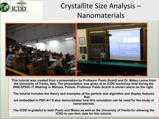
- 1. Crystallite Size Analysis – Nanomaterials This tutorial was created from a presentation by Professor Paolo Scardi and Dr. Mateo Leone from the University of Trento, Italy. The presentation was given at an ICDD workshop held during the 2008 EPDIC-11 Meeting in Warsaw, Poland. Professor Paolo Scardi is shown above on the right. The tutorial includes the theory and examples of the particle size algorithm and display features that are embedded in PDF-4+! It also demonstrates how this simulation can be used for the study of nanomaterials. The ICDD is grateful to both Paolo and Mateo as well as the University of Trento for allowing the ICDD to use their data for this tutorial. 1
- 2. Note This presentation can be directly viewed using your browser. It can also be saved, and viewed, with Microsoft® PowerPoint®. The authors have made additional comments in the notes section of this presentation, which can be viewed within PowerPoint®, but is not visible using the browser. 2
- 3. ICDD PDF-4+ 2008 EPDIC Workshop 3 Featuring: ICDD PDF-4+/DDView+ 2008: Applications to Nanomaterials Prof. Paolo Scardi (University of Trento), ICDD Director-at-Large Dr. Matteo Leoni (University of Trento), ICDD Regional Chair (Europe) September 19, 2008 3
- 4. PDF Card • Contains Diffraction Data of Material • Multiple d-Spacing Sets – Fixed Slit Intensity – Variable Slit Intensity – Integrated Intensity – New: Footnotes for d-Spacings (*) • Options – 2D/3D Structure – Bond Distances/Angles – Electron Patterns – New: PD3 Pattern – Diffraction Pattern 4
- 5. Diffraction Pattern • Simulated digitized pattern 5
- 6. Profile Settings • pseudo-Voigt (pV) • Modified Thompson- Cox-Hastings pV • Gaussian • Lorentzian • Particle Size 6
- 7. Diffraction Pattern • Particle Size (Gamma distribution of diameters of spherical coherent-scattering domains) Particle Size Particle Size 7
- 8. Profile Settings • pseudo-Voigt (pV) • Modified Thompson- Cox-Hastings pV • Gaussian ? Given the variety of available • Lorentzian profile functions, why bother with a new one??? • Particle Size Answer: because the size distribution matters!!! 8
- 9. PIONEERS IN POWDER DIFFRACTION: PAUL SCHERRER The Scherrer formula [Gottinger Nachrichten 2 (1918) 98] ln 2 λ h – full width at half maximum h=2 × Λ – effective domain size π Λ cos θ λ θ – – wavelength Bragg angle Paul Scherrer (1890–1969) Cerium oxide powder from xerogel, 1 h @400°C β= ∫ I ( 2θ ) d 2θ I ( 2θB ) 9
- 10. EFFECTIVE SIZE AND GRAIN SIZE What is the meaning of L, the ‘effective size’ of the Scherrer formula? λ β ( 2θ ) = L cos θ D 5 nm L ≠ D 10
- 11. SCHERRER FORMULA AND SIZE DISTRIBUTION In most cases, crystalline domains have a distribution of sizes (and shapes). Distribution ‘moments’ M i = ∫ D i g ( D)dD <D> = M1 mean M2 - M12 variance Scherrer formula is still valid λ 1 M4 β ( 2θ ) = → < L >V = < L >V cos θ Kβ M 3 Scherrer constant a shape factor, generally function of hkl (4/3 for spheres) 11
- 12. EFFECTS OF A SIZE DISTRIBUTION 1 M4 D L → < L >V = ≠ D Kβ M 3 5 nm Example: lognormal distributions of spheres, g(D) (mean µ , variance σ ) 12
- 13. EFFECTS OF A SIZE DISTRIBUTION Lognormal distribution of spheres: p ( D ) = exp − ( ln D − µ ) 2 ) 2σ 2 Dσ 2π D = 13.33 <L>V D = exp ( µ + σ 2 2 ) mean diameter < L >V = 3 4 exp ( µ + 7σ 2 2 ) ‘Scherrer’ size 13 P. Scardi, Size-Strain V (Garmisch (D) Sept. 2007). Z. Kristallogr. 2008. In press
- 14. EFFECTS OF A SIZE DISTRIBUTION Lognormal distribution of spheres: p ( D ) = exp − ( ln D − µ ) 2 ) 2σ 2 Dσ 2π D = 13.33 <L>V D = 13.23 D = exp ( µ + σ 2 2 ) mean diameter < L >V = 3 4 exp ( µ + 7σ 2 2 ) ‘Scherrer’ size 14 P. Scardi, Size-Strain V (Garmisch (D) Sept. 2007). Z. Kristallogr. 2008. In press
- 15. EFFECTS OF A SIZE DISTRIBUTION Lognormal distribution of spheres: p ( D ) = exp − ( ln D − µ ) 2 ) 2σ 2 Dσ 2π D = 13.33 <L>V D = 11.82 D = exp ( µ + σ 2 2 ) mean diameter < L >V = 3 4 exp ( µ + 7σ 2 2 ) ‘Scherrer’ size 15 P. Scardi, Size-Strain V (Garmisch (D) Sept. 2007). Z. Kristallogr. 2008. In press
- 16. EFFECTS OF A SIZE DISTRIBUTION Lognormal distribution of spheres: p ( D ) = exp − ( ln D − µ ) 2 ) 2σ 2 Dσ 2π D = 13.33 <L>V D = 8.25 D = exp ( µ + σ 2 2 ) mean diameter < L >V = 3 4 exp ( µ + 7σ 2 2 ) ‘Scherrer’ size 16 P. Scardi, Size-Strain V (Garmisch (D) Sept. 2007). Z. Kristallogr. 2008. In press
- 17. EFFECTS OF A SIZE DISTRIBUTION Lognormal distribution of spheres: p ( D ) = exp − ( ln D − µ ) 2 ) 2σ 2 Dσ 2π D = 13.33 <L>V D = 4.53 D = exp ( µ + σ 2 2 ) mean diameter < L >V = 3 4 exp ( µ + 7σ 2 2 ) ‘Scherrer’ size 17 P. Scardi, Size-Strain V (Garmisch (D) Sept. 2007). Z. Kristallogr. 2008. In press
- 18. EFFECTS OF A SIZE DISTRIBUTION Lognormal distribution of spheres: p ( D ) = exp − ( ln D − µ ) 2 ) 2σ 2 Dσ 2π D = 13.33 <L>V D = 1.95 D = exp ( µ + σ 2 2 ) mean diameter < L >V = 3 4 exp ( µ + 7σ 2 2 ) ‘Scherrer’ size 18 P. Scardi, Size-Strain V (Garmisch (D) Sept. 2007). Z. Kristallogr. 2008. In press
- 19. EFFECTS OF A SIZE DISTRIBUTION Lognormal distribution of spheres: p ( D ) = exp − ( ln D − µ ) 2 ) 2σ 2 Dσ 2π <L>V D = exp ( µ + σ 2 2 ) mean diameter < L >V = 3 4 exp ( µ + 7σ 2 2 ) ‘Scherrer’ size 19 P. Scardi, Size-Strain V (Garmisch (D) Sept. 2007). Z. Kristallogr. 2008. In press
- 20. EFFECTS OF A SIZE DISTRIBUTION Lognormal distribution of spheres: p ( D ) = exp − ( ln D − µ ) 2 ) 2σ 2 Dσ 2π D = exp ( µ + σ 2 2 ) mean diameter < L >V = 3 4 exp ( µ + 7σ 2 2 ) ‘Scherrer’ size 20 P. Scardi, Size-Strain V (Garmisch (D) Sept. 2007). Z. Kristallogr. 2008. In press
- 21. EFFECT OF A BIMODAL SIZE DISTRIBUTION If the size distribution is multimodal, a single (“mean size”) number is of little use, and possibly misleading!! 21
- 22. Profile Settings • pseudo-Voigt (pV) • Modified Thompson- Cox-Hastings pV • Gaussian • Lorentzian ? Given the variety of available profile functions, why bother • Particle Size with a new one??? Answer: because the size distribution matters!!! 22
- 23. “Particle size” option in DDView+ µ: mean σ: variance Gamma distribution ψ=πµs s=2sinθ/λ µ: mean σ: variance 23
- 24. “Particle size” option in DDView+ M. Leoni & P. Scardi, “Nanocrystalline domain size distributions 24 from powder diffraction data”, J. Appl. Cryst. 37 (2004) 629
- 25. “Particle size” option in DDView+ 25
- 26. “Particle size” option in DDView+ 26
- 27. “Particle size” option in DDView+ 27
- 28. “Particle size” option in DDView+ 28
- 29. “Particle size” option in DDView+ PDF 04-001-2097 cerium oxide PDF 04-001-2097 cerium oxide 29
- 30. “Particle size” option in DDView+ PDF 04-001-2097 cerium oxide 30
- 31. “Particle size” option in DDView+ PDF 04-001-2097 cerium oxide 31
- 32. “Particle size” option in DDView+ PDF 04-001-2097 cerium oxide 32
- 33. “Particle size” option in DDView+ PDF 04-001-2097 cerium oxide TEM: 4.5 nm XRD/WPPM:4.4nm M. Leoni & P. Scardi, “Nanocrystalline domain size distributions 33 from powder diffraction data”, J. Appl. Cryst. 37 (2004) 629
- 34. “Particle size” option in DDView+ Validating the procedure Diffraction pattern of Au generated by Debye equation 14000 1.0 Lognormal distribution of spherical domains (m=1.2, s=0.15) <D>=3.36 nm 12000 0.8 Frequency (a.u.) 10000 Intensity (a.u.) 0.6 8000 0.4 0.2 6000 0.0 4000 0 1 2 3 4 5 6 7 8 9 Spherical domain size (nm) 2000 0 20 30 40 50 60 70 80 90 100 2theta (deg) 34 K. Beyerlein, A. Cervellino, M. Leoni, R.L. Snyder & P. Scardi. EPDIC-11 (Warsaw (PL) Sept. 2008)
- 35. “Particle size” option in DDView+ 35
- 36. “Particle size” option in DDView+ 36
- 37. “Particle size” option in DDView+ 37
- 38. “Particle size” option in DDView+ 1.0 Lognormal (m=1.2, s=0.15) <D>=3.36 nm DDView+ Gamma (m=3.36, s=50) <D>=3.36 nm 0.8 Frequency (a.u.) 0.6 0.4 0.2 0.0 0 1 2 3 4 5 6 7 8 9 Spherical domain size (nm) 38
- 39. “Particle size” option in DDView+ 1.0 Lognormal (m=1.2, s=0.15) <D>=3.36 nm DDView+ Gamma (m=4.0, s=50) <D>=4.0 nm 0.8 Frequency (a.u.) 0.6 0.4 0.2 0.0 0 1 2 3 4 5 6 7 8 9 Spherical domain size (nm) 39
- 40. “Particle size” option in DDView+ 1.0 Lognormal (m=1.2, s=0.15) <D>=3.36 nm DDView+ Gamma (m=5.0, s=50) <D>=5.0 nm 0.8 Frequency (a.u.) 0.6 0.4 0.2 0.0 0 1 2 3 4 5 6 7 8 9 Spherical domain size (nm) 40
- 41. “Particle size” option in DDView+ 1.2 Lognormal (m=1.2, s=0.15) <D>=3.36 nm DDView+ Gamma (m=3.0, s=50) <D>=3.0 nm 1.0 Frequency (a.u.) 0.8 0.6 0.4 0.2 0.0 0 1 2 3 4 5 6 7 8 9 Spherical domain size (nm) 41
- 42. “Particle size” option in DDView+ 1.6 Lognormal (m=1.2, s=0.15) <D>=3.36 nm 1.4 DDView+ Gamma (m=2.0, s=50) <D>=2.0 nm 1.2 Frequency (a.u.) 1.0 0.8 0.6 0.4 0.2 0.0 0 1 2 3 4 5 6 7 8 9 Spherical domain size (nm) 42
- 43. “Particle size” option in DDView+ 1.0 Lognormal (m=1.2, s=0.15) <D>=3.36 nm DDView+ Gamma (m=3.36, s=50) <D>=3.36 nm 0.8 Frequency (a.u.) 0.6 0.4 0.2 0.0 0 1 2 3 4 5 6 7 8 9 Spherical domain size (nm) 43
- 44. “Particle size” option in DDView+ CAVEAT! • DDView+ “Particle size” is NOT a profile fitting! • NO other sources of line broadening (e.g., instrumental profile, dislocations, etc.) are considered! • Gamma distribution is flexible and handy, but in some cases it MIGHT NOT work! Domains might not be spherical! Use this feature only for estimating domain size, especially in nano materials where the line width/shape is dominated by the size effects. In all other cases, use a Line Profile Analysis software, e.g., PM2K, based on the WPPM algorithm (Paolo.Scardi@unitn.it) 44
- 45. Thank you for viewing our tutorial. Additional tutorials are available at the ICDD web site ( www.icdd.com). International Centre for Diffraction Data 12 Campus Boulevard Newtown Square, PA 19073 Phone: 610.325.9814 Fax: 610.325.9823 45
Notas del editor
- This talk is given to explain the ‘’Particle Size’’ feature in DDView+. Basic theory is presented, also to explain why it can be useful to use this feature with respect to ‘standard’ profile functions, commonly used in most PD software
- This and the following 4 slides are taken from the ‘’Getting Started’’ talk. It is shown how to generate the powder pattern from a PDF card. Then profile setting are discussed, in particular the available profile shape functions.
- .
- .
- .
- This slide is to introduce the main point of the talk: why introducing this feature in DDView+ ? Answer is, as shown in the following, that size distribution effects may be important in Powder Diffraction, especially when dealing with nanosize powders (i.e., below 100 nm)
- Line Profile Analysis (LPA), as it is nowadays called the study of powder diffraction peak profiles, was first introduced by Scherrer, as early as in 1918. The Scherrer formula shows the inverse proportionality between effective domain size and peak width. Peak width can be given by Full Width at Half Maximum (FWHM), but is better represented by the integral breadth (beta=peak area/peak maximum intensity)
- What is the ‘’effective domain size’’ ? Is it equivalent or somehow related to the ‘’grain size’’ that one might observe in a microscopy. The general answer to the last question is: no they are generally different.
- In most cases the size of coherently scattering domains (that we also call crystallites) is not the same throughout the powder specimen. The size most likely is ‘dispersed’: provided that domains have (at least approximately) a given shape, the size parameter (e.g. diameter for a sphere) is spread according to some distribution g(D). The Scherrer equation still holds, but the effective size is a rather complex average of the actual domain size: <L>v is proportional to the ratio between 4-th and 3-rd distribution Moments (Mi). The proportionality constant (Scherrer constant, Kb) is in general a function of hkl. A special case is valid for spheres, for which Kb is 4/3 for all hkls. ( 1° moment is the arithmetic mean, <D>, also written as D with overbar)
- Here we can see the effect of a size distribution. In some cases <L>v (aka Scherrer size) is close to the arithmetic mean size (that we might think to obtain, for example, by microscopy). This is the case of the distribution on the left, which is narrow and symmetrical. In most cases, however, the Scherrer size is of little use or doubtful meaning. Nothing wrong in evaluating <L>v, but one might easily miss the point !! See the large difference between <L>v and <D> for the skewed distribution on the right.
- To further illustrate this important point, the following slides show a set of simulated patterns for a powder of spherical domains with a lognormal distribution of diameters. All patterns have the same Scherrer size (= 10 nm), but totally different size distribution. How can we obtain such a condition? Using known expressions relating lognormal mean (mu), variance (sigma), mean domain size (<D>) and Scherrer size (<L>v), the latter can be kept constant while changing mu and sigma.
- Here we see the pattern (nearly equal to the previous one) for a slightly broader distribution (remember that Scherrer size is the same!).
- Again, same Scherrer size, but broader distribution: difference between patterns are now visible.
- Broader distribution, more marked differences in the patterns
- One more.
- Last example of the series. The Scherrer size is still fixed to 10 nm, but corresponds to a skewed distribution, with an arithmetic mean of less than 2 nm. The diffraction pattern is markedly different from that of the first example (the narrow distribution with <D>=13.33 nm).
- All simulations shown together. It is worth underlying that all peak profiles have the same peak width (strictly speaking, same integral breadth), as they are simulated using the same Scherrer size of 10 nm, but they refer to completely different size distributions. Peak shape is clearly different.
- To summarize, patterns where simulated with constant Scherrer size and different values of <D> and sigma. This should make evident that quoting a single number, the Scherrer size, is in most cases not correct: features of the size distribution are also important and influence the peak shape.
- If the size distribution is bimodal (or multimodal in the most general case), the vary concept of ‘mean size’, whether we refer to <D> or to <L>v, is of little use. As a general rule, the Scherrer size tends to give more weight to the fraction of larger crystallites. This is an effect of the ratio between high order moments (M4/M3).
- In conclusion: size distribution matters !
- Some elements of theory: details in the cited paper. The ‘’Particle Size’’ option of DDView+ assumes spherical crystallites with a Gamma distribution of diameters. Gamma distribution is convenient: (1) it is described by two parameters (variance (sigma) and mean (mu)) with a clear meaning, (2) and it is sufficiently flexible to approximate most real cases. Extreme shapes are an exponential (for sigma=1) and a Gaussian (for large values of sigma). As shown here, the peak profile function is a function of mu and sigma (and lambda, thw X-ray wavelength). When we enter ‘’Mean particle diameter’’ and ‘’Particle Variance’’ in DDView+ window ‘’Profile’’, we enter respectively mu and sigma.
- First example. This is a real case of study. The pattern shown here was collected by a standard laboratory instrument and refers to a nanocrystalline powder of cerium oxide produced by the sol-gel method. The pattern here shown is for a xerogel heat treated at 400°C for 1 hour. Peaks are broad but clearly show the material is well crystallized. TEM confirms this information, and also shows that particles are single crystal with nearly spherical shape. In this case – and this is an important point – the main reason for diffraction peak profile broadening is the small size of the crystals. Additional broadening is given by the instrument and lattice defects. However, we can expect the contribution of those additional line broadening source to be relatively small
- So we use the PDF-4+ and DDView+, first to retrieve a cerium oxide card. Here we wish to select the Primary card of stoichiometric CeO2, and we wish to see the full structural information (04-XXX-XXXX cards)
- So we use the PDF-4+ and DDView+, first to retrieve a cerium oxide card. Here we wish to select the Primary card of stoichiometric CeO2, and we wish to see the full structural information (04-XXX-XXXX cards)
- So we use the PDF-4+ and DDView+, first to retrieve a cerium oxide card. Here we wish to select the Primary card of stoichiometric CeO2, and we wish to see the full structural information (04-XXX-XXXX cards)
- So we use the PDF-4+ and DDView+, first to retrieve a cerium oxide card. Here we wish to select the Primary card of stoichiometric CeO2, and we wish to see the full structural information (04-XXX-XXXX cards)
- The Primary card for stoichiometric CeO2 is 04-001-2097.
- We now generate the diffraction pattern (the peak profile is pseudoVoigt for starting; peaks are narrow). We then import the experimental data for the cerium oxide nanopowder (file is in the form of a two column datafile (.xy)).
- It is then convenient, just to the purpose of a better match, to remove the background. Always mind the Grid Size and Repeats: when removing a background from a pattern with broad profiles one should try not to remove part of the signal. As a general rule, when deailing with experimental data in more quantitative applications (so, not for the present case!) one should always avoid removing background and/or smooth the data.
- Once the background has been removed, we go to ‘’Edit’’ / ‘’Preferences’’ and select ‘’Profile’’. There we change from pseudoVoigt to Particle size and enter some tentative values. Peak tails are important in this application, so we extend the value of Significance limit to 0.001 or less. After some attempts, by trial and error we get to mu = 40 and sigma = 6
- With mu = 40 and sigma = 6 the match between DDView+ simulation and experimental data is very good. It is also interesting to compare the result (mean size 4.0 nm) with the result obtained by TEM (4.5 nm, green histogram) and by a more general, complete and robust Line Profile Analysis software (PM2K, based on the Whole Powder Pattern Modelling algorithm, University of Trento) (4.4 nm). The agreement between the result obtained by DDView+ and the other results is within 10%, so it is quite good. It is worth noting that: (1) DDView+ is NOT a fitting/modelling software; the result was obtained by manually change parameters, so it cannot be the best; (2) differences are expected in this case: there is additional (although little) broadening due to the instrument and to lattice defects (dislocations), which is not considered by DDView+. As a consequence DDView+ always tends to (slightly) underestimate the domain size, and should only be used when the main (if not th eonly) source of line broadening is that of the small domain size.
- As an additional, much convincing example, we now consider data for a powder of gold nanocrystals, with spherical domains and lognormally distributed diameters. In this case the powder diffraction pattern was obtained by a simulation based on the Debye equation, which is the most ‘exact’ expression one can use for nanocrystals. It is interesting to verify what one can obtain using DDView+, also considering that DDView+ adopts a Gamma distribution, whereas the simulated data are obtained for a lognormal distribution. It is worth underlying that the distribution,m in the here considered, is rather symmetrical.
- We now retrieve the Primary card of Gold from the PDF-4+
- We now retrieve the Primary card of Gold from the PDF-4+
- Following the same procedure shown before, we import the gold pattern (as a .xy file). Then we change the profile function, originally a narrow pseudoVoigt profile function, to Particle Size and use: mu=33.6, that is the same mean size as in the lognormal used to simulate the data; sigma=50, which gives a nearly Gaussian distribution (in general, a narrow/symmetrical distribution).
- The result is remarkably good. The match cannot be ‘perfect’ because: (1) size ditribution is intrinsically different (Lognormal for simulate ddata, Gamma for DDView+); (2) some additional features should be considered: for example, the Small Angle X-ray Scattering (SAXS) oscillating ‘tail’ which is responsible for an apparently high background in the simulated data; (3) also the unit cell parameter is not exactly that of the PDF-4+ card. In spite of all those fine differences, the match is very good, also for the size distributions, that look pretty similar.
- We can see what happens if we slightly change the mean size, from <D> (=mu) = 3.36 nm to 4.00 nm. The DDView+ pattern now is clearly narrower. Even a small change is clearly visible: in this range of values (from a few nm to tens of nm) powder diffraction is very sensitive.
- Differences are more evident when we increase the mean size to 5.0 nm.
- We can also verufy the difference in line profiles when the mean size in DDView+ is decreased to a mean size of 3.0 nm. Even with such a small difference with respect to the correct value (3.36 nm) used to produce the simulated data, the diffraction pattern is clearly different
- A further decrease in mean size do 2.0 nm gives a much broader line profile, and the patter is clearly different from the simulate data. Once more we see how sensitive is powder diffraction.
- In conclusion …
- To conclude, we have shown that the ‘’Particle Size’’ option of DDView+ is simple to use and it works fine for a quick estimate of the domain size. However, it cannot substitute a more exhaustive evaluation of each case of study, by means of more robust modelling algorithms and other techniques. People interested in line profile analysis can contact: [email_address]