Need to understand Six Sigma and productivity charts? See this presentation to learn about C and U charts.

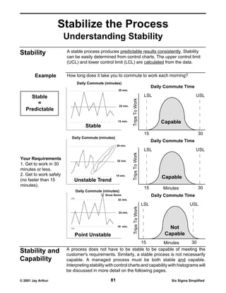
1. Stabilize the Process
Understanding Stability
Stability A stable process produces predictable results consistently. Stability
can be easily determined from control charts. The upper control limit
(UCL) and lower control limit (LCL) are calculated from the data.
Example How long does it take you to commute to work each morning?
Daily Commute (minutes)
Daily Commute Time
29 min.
Stable LSL USL
Trips To Work
= 22 min.
Predictable
15 min. Capable
Stable
15 30
Daily Commute (minutes)
Daily Commute Time
29 min.
LSL USL
Trips To Work
Your Requirements 22 min.
1. Get to work in 30
minutes or less.
2. Get to work safely 15 min.
Capable
(no faster than 15 Unstable Trend
minutes).
15 Minutes 30
Daily Commute (minutes)
Snow Storm Daily Commute Time
UCL
32 min.
LSL USL
Trips To Work
24 min.
LCL
18 min.
Not
Point Unstable Capable
15
Minutes 30
A process does not have to be stable to be capable of meeting the
Stability and customer's requirements. Similarly, a stable process is not necessarily
Capability capable. A managed process must be both stable and capable.
Interpreting stability with control charts and capability with histograms will
be discussed in more detail on the following pages.
© 2001 Jay Arthur 81 Six Sigma Simplified

2. Check Stability
Interpreting The Indicators
Purpose Verify that the process system is stable and
can predictably meet customer requirements
Variation A stable process produces predictable results. Understanding
variation helps us learn how to predict the performance of any
You cannot step process. To ensure that the process is stable (i.e., predictable)
twice into the same
we need to develop "run" or "control" charts of our indicators.
river.
Heraclitus How can you tell if a process is stable? Processes are never
perfect. Common and special causes of variation make the
process perform differently in different situations. Getting from
your home to school or work takes varying amounts of time
because of traffic or transportation delays. These are common
causes of variation; they exist every day. A blizzard, a traffic
accident, a chemical spill, or other freak occurrence that causes
major delays would be a special cause of variation.
In the 1920s, Dr. Shewhart, at Bell Labs, developed ways to
evaluate whether the data on a line graph is common cause or
special cause variation. Using 20-30 data points, you can
determine how stable and predictable the process is. Using
simple equations, you can calculate the average (center line),
and the upper and lower "control limits" from the data. 99% of
all expected (i.e., common cause variation) should lie between
these two limits. Control limits are not to be confused with
specification limits. Specification limits are defined by the cus-
Example tomer. Control limits show what the process can deliver.
Your Requirements:
1. Get to work fast! Upper Control Limit (UCL)
2. Get to work safely.
Daily Commute (minutes)
68.3%
95.5%
99.7% of all
29 min. Center Line (average) data points
22 min.
Lower Control Limit (LCL)
15 min.
1 5 10 15 20 25 30
Stable
© 2001 Jay Arthur 82 Six Sigma Simplified

3. Check Stability
Interpreting The Indicators
Special Processes that are "out of control" need to be stabilized before
they can be improved using the problem-solving process.
Cause Special causes, require immediate cause-effect analysis to
Variation eliminate the special cause of variation.
Evaluating The following diagram will help you evaluate stability in any
control chart. Unstable conditions can be any of the following:
Stability
Any point above UCL
UCL
2 of 3 points in this area
Daily Commute (minutes)
Snow Storm 4 of 5 points in this area or above
29 min.
8 points in a row in this area or above
CL
22 min. 8 points in a row in this area or below
4 of 5 points in this area or below
15 min.
2 of 3 points in this area
Point Unstable LCL
Any point below LCL
1 5 10 15 20 25 30
Points and Any point outside the upper or lower control limits is a clear
example of a special cause. The other forms of special cause
Runs
variation are called "runs." Trends, cycling up and down, or
"hugging" the center line or limits are special forms of a run.
Point outside UCL
UCL
2 above A 8 above CL
A
Daily Commute (minutes)
29 min.
B
CL
22 min.
Trend B
15 min.
4 below B 6 ascending A
Unstable Trend or descending
LCL
Any point below LCL
© 2001 Jay Arthur 83 Six Sigma Simplified

4. Step 4 - Check Stability
c and u charts
c and u The c and u charts will help you evaluate process stability when
Charts there can be more than one defect per unit. Examples might
include: the number of defective elements on a circuit board, the
(Attribute data)
number of defects in a dining experience–order wrong, food too
cold, check wrong, or the number of defects in bank statement,
X X invoice, or bill. This chart is especially useful when you want to
X know how many defects there are not just how many defective
items there are. It's one thing to know how many defective circuit
Defects boards, meals, statements, invoices, or bills there are; it is
another thing to know how many defects were found in these
defective items.
The c chart is useful when it's easy to count the number of
defects and the sample size is always the same. The u chart is
used when the sample size varies: the number of circuit boards,
meals, or bills delivered each day varies. The c chart below
shows the number of defects per day in a uniform sample.
Number Defects Per Day
n=28
7 Point Outside Limits
To automate all of 6
UCL
your control charts
Number of Defects
5
using Microsoft®
4
Excel, get the
QI Macros For Excel. 3
Download a FREE 2 Run Below CL
CL
limited demo from:
1
www.quantum-i.com Approach to Limits Approach to Limits
0 LCL
10-Feb
11-Feb
12-Feb
13-Feb
14-Feb
15-Feb
16-Feb
17-Feb
18-Feb
19-Feb
20-Feb
21-Feb
22-Feb
23-Feb
24-Feb
25-Feb
26-Feb
27-Feb
28-Feb
1-Feb
2-Feb
3-Feb
4-Feb
5-Feb
6-Feb
7-Feb
8-Feb
9-Feb
Stability Given this information, we would want to investigate why
February 11th was "out of control." We would also want to
understand why we were able to keep the defects so far below
average in the other circled areas. What did we do here that was
so successful?
Capability A fully capable process delivers zero defects.
© 2001 Jay Arthur 90 Six Sigma Simplified

5. Step 4 - Check Stability
c and u charts
X X = More Than
X One Defect
Title
Number
or Percent
of Defects
1 2 3 4 5 6 7 8 9 10 11 12 13 14 15 16 17 18 19 20
Measurement or Sample
c 1 2 3 4 5 6 7 8 9 10 11 12 13 14 15 16 17 18 19 20
Defects (c)
u 1 2 3 4 5 6 7 8 9 10 11 12 13 14 15 16 17 18 19 20
Defects (u)
Sample Size (n)
Percent
UCL
LCL
C Chart U Chart
UCL: c + 3*sqrt(c) u + 3*sqrt(u/n )i
CL: c = ∑ci/n u = ∑ui/∑ni
LCL: c - 3*sqrt(c) u - 3*sqrt(u/n )
i
© 2001 Jay Arthur 91 Six Sigma Simplified