weak introduction

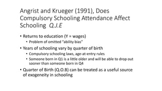
1. Angrist and Krueger (1991), Does
Compulsory Schooling Attendance Affect
Schooling Q.J.E
• Returns to education (Y = wages)
• Problem of omitted “ability bias”
• Years of schooling vary by quarter of birth
• Compulsory schooling laws, age-at-entry rules
• Someone born in Q1 is a little older and will be able to drop out
sooner than someone born in Q4
• Quarter of Birth (Q.O.B) can be treated as a useful source
of exogeneity in schooling

2. Angrist and Krueger (1991), Q.J.E.
People born in Q1 do obtain
less schooling
• But pay close attention to
the scale of the y-axis
• Mean difference between
Q1 and Q4 is only 0.124, or
1.5 months
So...need large N since R2
X,Z
will be very small
• A&K had over 300k for the
1930-39 cohort
Source: Angrist and Krueger (1991), Figure I

3. Angrist and Krueger (1991), Q.J.E.
Final 2SLS model interacted QOB with year of birth (30),
state of birth (150)
• OLS: b = .0628 (s.e. = .0003)
• 2SLS: b = .0811 (s.e. = .0109)
Least squares estimate does not appear to be badly
biased by omitted variables
• But...replication effort identified some pitfalls in this
analysis that are instructive

4. Weak instrument bias in IV estimators
• The graduate labor class at the University of Michigan does
replication exercises. (Moderately short papers).
• Regina Baker and David Jaeger manage to replicate the
results (Angrist and Krueger shared the data).
• But two things bother them and Prof. Bound:
• (Tables 1 and 2).

5. Angrist and Krueger (1991), J.L.E.
• People born in Q1 do
obtain less schooling
• But pay close attention to
the scale of the y-axis
• Mean difference between
Q1 and Q4 is only 0.124,
or 1.5 months
• So...need large N since
R2
X,Z will be very small
• A&K had over 300k for the
1930-39 cohort Source: Angrist and Krueger (1991), Figure I
Small Sample Bias of IV Estimators
Worry #1: The results are imprecise and unstable when the controls and instrument
sets change.

6. Angrist and Krueger (1991), J.L.E.
• Final 2SLS model interacted QOB with year of
birth (30), state of birth (150)
• OLS: b = .0628 (s.e. = .0003)
• 2SLS: b = .0811 (s.e. = .0109)
• Least squares estimate does not appear to be
badly biased by omitted variables
• But...replication effort identified some pitfalls in this
analysis that are instructive
Small Sample Bias of IV Estimators
Worry #1: The results are imprecise and unstable when the controls and instrument
sets change.
Small Sample Bias of IV Estimators
Worry #2:
The results become
precise and stable
only when the first
stage F tests cannot
reject coefficients
which are jointly
zero.

7. Bound, Jaeger, and Baker (1995), J.A.S.A.
• Potential problem with quarter of birth as an IV
• Lots of instruments and the correlation between QOB
and schooling is weak (weak instrument problem)
• Small Cov(X,Z) introduces finite-sample bias, which will be
exacerbated with the inclusion of many IV’s
• IV is biased but consistent: while the asymptotics are fine, we have some
bias in finite samples. It turns out that this bias in finite samples is worse
when we have weak instruments (with the bias being towards the OLS β).
• The form of this bias is generally well approximated by
1/(F+1)
• Where F is the population analogue of the F-statistic for the joint
significance of the instruments in the first stage regression.
See Mostly Harmless Econometrics pp. 206-208 for a derivation.

8. Small (finite) sample bias
• Consider the first stage:
x = zδ + ω.
• Even if δ=0 in the population, as the number of instruments
increases the R2 of the first stage regression in the sample can
only increase.
• As we add instruments, x hat approximates x better and better,
so that the 2nd stage IV estimate converges to the OLS estimate.
• When IVs are weak, adding more weak IVs will make the problem worse, as this will
diminish the F but not the covariance of unobservables
• To show this Bound, Jaeger and Baker replicate Angrist and
Krueger using random numbers as instruments!
• They get back the OLS estimates

9. Bound,
Jaeger, and Baker (1995),
J.A.S.A.
• Even if the instrument is “good,” matters can
be made far worse with IV as opposed to LS
• Weak correlation between IV and endogenous
regressor can pose severe finite-sample bias
• And…really large samples won’t help, especially if there
is even weak endogeneity between IV and error
• First-stage diagnostics provide a sense of how
good an IV is in a given setting
• F-test and partial-R2 on IV’s
Simulation with a random instrument
As an illustration, B,B and J
estimated the IV coefficient with
a randomly assigned Z so that
δ=0 by construction.
They did a great job reproducing
the OLS estimate.

10. What to do about weak instruments?
• Diagnostics based on the F-test for the joint significance of
the IV’s
• Nelson and Startz (1990); Staiger and Stock (1997)
• Bound, Jaeger, and Baker (1995)
• Rule of Thumb F-Stat should be greater than 10
• If you have many IVs pick your best instrument and report
the just identified model
• Look at the Reduced Form!
• The reduced form is estimated with OLS and is therefore
unbiased.
• If you can’t see the causal relationship of interest in the reduced form it is
probably not there.

11. Bound, Jaeger, and Baker (1995), J.A.S.A.
• Potential problems with quarter of birth as an IV
• Quarter of Birth may not be completely exogenous (i.e there may be a
(very?) small correlation between Z and e)
• Why might quarter of birth be correlated with the residual in
the earnings equation?
• Age at entry (being older than your classmates is good for self
confidence and sport participation)
• Season of birth (lower birthweights; teachers give birth in the
summer)
• Normally we wouldn’t worry much about these small sources of bias -
They pass the overidentification test.
• Even small Cov(Z,e) will cause inconsistency, and this will be
exacerbated when Cov(X,Z) is small

12. Bound, Jaeger, and Baker (1995), J.A.S.A.
• It turns out that if you have a weak instrument and an
imperfect (but still pretty good) instrument the IV estimate
can be quite biased. In fact the IV estimate might be more
biased than the OLS estimate
• Asymptotic behavior of IV
plim(bIV) = β + Cov(Z,e) / Cov(Z,X)
• If Z is truly exogenous, then Cov(Z,e) = 0 so no problem
• However if Cov(Z,X) is small, even a small Cov(Z,e) can lead to a
very biased IV estimate.
• In this example we may be latching onto the kids with higher wages because
of ,say, sport participation or high self-confidence.

13. Suppose our instrument is not truly exogenous i.e.
Cov(Z,ε) ̸= 0.
• Consider the example of difference in wages (Y) due to serving in the
Vietnam War(X), using the draft lottery number (Z) as an instrument. We
know that the OLS estimator E(Y |X = 1) − E(Y |X = 0) is biased, because
serving in the army is correlated with lots of unobserved characteristics.
• For the IV Wald estimator, the denominator represents the difference in
the probability of serving in the army for people with high and low lottery
numbers i.e. this number is less than 1.
• Suppose in fact the draft lottery number were not random, then E(Y |Z = 1)
− E(Y |Z = 0) is a biased estimate of the reduced form impact of lottery
number on wages. Notice now that even if the bias in the reduced form is
of the same order of magnitude as the bias of OLS, the IV estimate as a
whole is much more biased, because the denominator is less than one.