The GRASS GIS software (with QGIS) - GIS Seminar
•Descargar como ODP, PDF•
40 recomendaciones•16,845 vistas

Introduction to GRASS and QGIS for newbies, 6 hours course with practical examples based on GRASS 6 and QGIS
![GRASS: Geographic Resources Analysis Support System ,[object Object],[object Object],[object Object]](data:image/gif;base64,R0lGODlhAQABAIAAAAAAAP///yH5BAEAAAAALAAAAAABAAEAAAIBRAA7)
Recomendados
Más contenido relacionado
La actualidad más candente
La actualidad más candente (20)
Similar a The GRASS GIS software (with QGIS) - GIS Seminar
Similar a The GRASS GIS software (with QGIS) - GIS Seminar (20)
Más de Markus Neteler
Más de Markus Neteler (17)
Último
Último (20)
The GRASS GIS software (with QGIS) - GIS Seminar
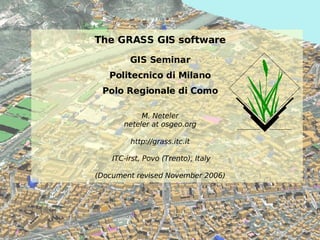
- 1. The GRASS GIS software GIS Seminar Politecnico di Milano Polo Regionale di Como M. Neteler neteler at osgeo.org http://grass.itc.it ITC-irst, Povo (Trento), Italy (Document revised November 2006)
- 4. GRASS GIS Brief Introduction Developed since 1984, always Open Source , since 1999 under GNU GPL Written in C programming language, portable code (multi-OS, 32/64bit) International development team , since 2001 coordinated at ITC-irst GRASS master Web site: http://grass.itc.it GNU/Linux MacOSX MS-Windows iPAQ
- 6. Spatial Data Types Supported Spatial Data Types 2D Raster data incl. image processing 3D Voxel data for volumetric data 2D/3D Vector data with topology Multidimensional points data http://grass.itc.it Orthophoto Distances Vector TIN 3D Vector buildings Voxel
- 7. Raster data model Raster geometry cell matrix with coordinates resolution: cell width / height (can be in kilometers, meters, degree etc.) y resolution x resolution
- 8. Vector data model Vector geometry types Point Centroid Line Boundary Area (boundary + centroid) face (3D area) [kernel (3D centroid)] [volumes (faces + kernel)] Geometry is true 3D: x, y, z Line Faces not in all GIS! Node Node Vertex Vertex Segment Segment Segment Node Boundary Vertex Vertex Vertex Vertex Centroid Area
- 9. OGC Simple Features versus Vector Topology Simple Features ... - points, lines, polygons - replicated boundaries for adjacent areas Advantage: - faster computations Disadvantage: - extra work for data maintenance - in this example the duplicated boundaries are causing troubles Switzerland slivers Map generalized with Douglas-Peucker algorithm in non-topological GIS gaps (Latitude-longitude)
- 10. OGC Simple Features versus Vector Topology ... versus Vector Topology - points, centroids, lines, boundaries - in topology centroid and boundary form an area - single boundaries for adjacent areas Advantage: - less maintenance, high quality Disadvantage: - slower computations Switzerland Original Pruned each boundary is a single line, divided by two polygons (UTM32N projection) Map generalized with v.clean “prune” algorithm in topological GIS GRASS
- 11. Italy: Gauss-Boaga Coordinate System Gauss-Boaga Transverse Mercator projection 2 zones ( fuso Ovest, Est ) with a width of 6º30' longitude Each zone is an own projection! False easting: Fuso Ovest: 1500000m (1500km) Fuso Est: 2520000m (2520km) False northing: 0m Scale along meridian: 0.9996 – secante case, not tangent case Ellipsoid: international (Hayford 1909, also called International 1924) Geodetic datum : Rome 1940 (3 national datums; local datums to buy from IGM). National datum values available at: http://crs.bkg.bund.de/crs-eu/
- 12. Italy: Gauss-Boaga Fuso Ovest ESRI PRJ-File for Fuso Ovest (g.proj -w in GRASS) PROJCS[" Monte_Mario_Italy_1 ", GEOGCS[" GCS_Monte_Mario ", DATUM[" Monte_Mario ", SPHEROID[" International_1924 ", 6378388 , 297 ]], PRIMEM[" Greenwich ", 0 ], UNIT[" Degree ", 0.017453292519943295 ]], PROJECTION[" Transverse_Mercator "], PARAMETER[" False_Easting ", 1500000 ], PARAMETER[" False_Northing ", 0 ], PARAMETER[" Central_Meridian ", 9 ], PARAMETER[" Scale_Factor ", 0.9996 ], PARAMETER[" Latitude_Of_Origin ", 0 ], UNIT[" Meter ", 1 ]] EPSG codes: Gauss-Boaga/Monte Mario 1: EPSG 26591 Gauss-Boaga/Monte Mario 2: EPSG 26592
- 13. Geodetic Datums of Gauss-Boaga Geodetic datum: “peninsular datum” "Monte Mario to WGS 84 (4)","Position Vector 7-param. transformation", "X-axis translation","1","-104.1","metre","Italy - mainland" "Y-axis translation","2","-49.1","metre","Italy - mainland" "Z-axis translation","3","-9.9","metre","Italy - mainland" "X-axis rotation","4","0.971","arc-second","Italy - mainland" "Y-axis rotation","5","-2.917","arc-second","Italy - mainland" "Z-axis rotation","6","0.714","arc-second","Italy - mainland" "Scale difference","7","-11.68","parts per million","Italy - mainland" also available: Sardegna, Sicilia
- 14. How to use GRASS GIS? GRASS startup screen
- 15. GRASS: Modernized GIS manager and WMS support gis.m: Michael Barton, Cedric Shock r.in.wms: Sören Gebbert & Jachym Cepicky
- 16. GRASS integration with QGIS http://qgis.org QGIS-GRASS plugin: Radim Blazek
- 17. WebGIS: Integration of data sources GRASS in the Web Real-time monitoring of Earthquakes (provided in Web by USGS) with GRASS/PHP: http://grass.itc.it/spearfish/php_grass_earthquakes.php
- 18. GRASS GIS Interoperability Data models and formats
- 19. WebGIS: Integration of data sources GIS – DBMI – Mapserver linking WMS/WFS/WMC/SLD Raster: GeoTIFF, IMG, ... Vector: SHAPE, MapInfo,... PostGIS ArcSDE Oracle Sp. Raster Vector/DBMI GRASS
- 23. Spearfish Sample Dataset Spearfish (SD) sample data location Maps: raster, vector and point data covering two 1:24000 topographic maps (quadrangles Spearfish and Deadwood North) UTM zone 13N, transverse mercator projection, Clarke66 ellipsoid, NAD27 datum, metric units, boundary coordinates: 4928000N, 4914000S, 590000W, 609000E DATA download: http://mpa.itc.it/markus/osg05/ SD Spearfish
- 24. Practical GIS Usage Start a “terminal” to enter commands Start GRASS 6 within the terminal: grass61 -help grass61 -gui 1. 2. 3.
- 25. GRASS user interface: QGIS Start QGIS within GRASS terminal: qgis http://qgis.org GRASS Toolbar
- 26. QGIS: further key functionality Creating a paper map GRASS toolbox GRASS raster maps GRASS vector maps GRASS vector digitizer
- 27. New GRASS user interface: QGIS Excercise: Please reproduce this map view! Raster: - elevation.dem - aspect Vector: - roads - fields
- 28. QGIS map composer: prepare map with layout Creating a paper map for printing or saving into a file (SVG, PNG, Postscript) Transfer map view into map composer (printer symbol)
- 29. QGIS: further key functionality Vector map visualization Raster map viz. PostGIS map viz. WMS viz. Map query Vector object selection Attribute table
- 30. QGIS: GRASS toolbox GRASS toolbox
- 31. QGIS-GRASS Exercises: Noise impact 1/4 1) Simple noise impact map: Extract interstate (highway) from roads vector map into new map and buffer interstate for 3km in each direction GRASS commands: a) first look at the table to get column name and ID of interstate: v.db.select roads b) we extract only 'interstate' (cat = 1, cat is the GRASS standard column name for ID): v.extract in=roads out=interstate where=”cat = 1” c) we buffer the interstate (give buffer in map units which is meters here): v.buffer interstate out=interstate_buf3000 buffer=3000
- 32. QGIS-GRASS Exercises: Noise impact 2/4 2) Verify affected areas: Look at landcover.30m raster map, overlay extracted interstate and overlay buffered interstate_buf3000 (use transparency to make it nice)
- 33. # set current region to landcover map, '-p' prints the settings: g.region rast= landcover.30m -p Info: Command line versus graphical user interface On the next slide we either use the following command line: or these settings in the graphical user interface:
- 34. QGIS-GRASS Exercises: Noise impact 3/4 How to get statistics on influenced landcover-landuse units? -> needs generalization of original landcover.30m map (originates from satellite map) Approach 1: Raster based generalization : “mode” operator in moving window # set current region to landcover map, '-p' prints the settings: g.region rast= landcover.30m -p r.neighbors in= landcover.30m out= landcover.smooth method= mode size= 3 3x3 moving window
- 35. QGIS-GRASS Exercises: Noise impact 4/4 ... Generalization cont'ed: Approach 2: Vector based generalization : “rmarea” tool: merges small areas into bigger a. # zoom to map: g.region rast= landcover.30m -p # raster to vector conversion: r.to.vect in= landcover.30m out= landcover_30m f=area # filter perimeter of 3x3 pixels ( threshold=(30 * 3)^2 = 8100) v.clean in= landcover_30m out= landcover_30m_gen tool= rmarea thresh= 8100
- 36. Perspective view of maps nviz el=elevation.dem vect=roads
- 38. GRASS: Geographic Resources Analysis Support System Example for Location and Mapsets /home/user/grassdata /europa /hannover /world hist dbln coor sidx topo Mapset Location /PERMANENT GRASS Database /prov_trentino /PERMANENT /trento Geometry and attribute data streets parks lakes poi streets.dbf parks.dbf poi.dbf lakes.dbf fcell hist colr cell_misc cellhd cell cats vector dbf /silvia
- 39. Raster map analysis DEM analysis Raster map algebra Geocoding of scanned map Volume data processing
- 40. GRASS Command Classes d.* display graphical output (screen) r.* raster raster data processing r3.* raster3D raster voxel 3D data processing i.* imagery image processing v.* vector vector data processing g.* general general file operations (copy, rename of maps, ...) m.* misc miscellaneous commands ps.* postscript map creation in Postscript format Prefix Class Functionality
- 42. Raster data analysis: Geomorphology DEM: r.param.scale # set region/resolution to the input map: g.region rast=elevation.10m -p # generalize with size parameter r.param.scale elevation.10m out=morph param=feature size=25 # with legend d.rast.leg morph # view with aspect/shade map (or QGIS) d.his h=morph i=aspect.10m Spearfish DEM: 10m Moving window size: 25x25 nviz elev=elevation.10m col=morph
- 43. Raster data analysis: Water flows - Contributing area Topographic Index: ln(a/tan(beta)) g.region rast=elevation.10m -p r.topidx in=elevation.10m out=ln_a_tanB d.rast ln_a_tanB d.vect streams col=yellow # ... the old vector stream map nicely deviates from the newer USGS DEM nviz elevation.10m col=ln_a_tanB
- 47. Working with vector data Vector map import Attribute management Buffering Extractions, selections, clipping, unions, intersections Conversion raster-vector and vice verse Digitizing in GRASS and QGIS Working with vector geometry
- 48. GRASS 6 Vector data Vector geometry types Point Centroid Line Boundary Area (boundary + centroid) face (3D area) [kernel (3D centroid)] [volumes (faces + kernel)] Geometry is true 3D: x, y, z Line Faces Node Node Vertex Vertex Segment Segment Segment Node Boundary Vertex Vertex Vertex Vertex Centroid Area
- 49. Raster-Vector conversion – extraction 1/2 Extraction of residential areas from raster landuse map # set current region to map; look at the landuse/landcover map with legend: g.region rast=landcover.30m -p d.erase d.rast.leg -n landcover.30m # Automated vectorization of the landuse/landcover map: r.to.vect -s landcover.30m out=landcover30m feature=area # see attribute table ('-p' prints the current connection between vector # geometry and attribute table – note that GRASS can link to various DBMS): v.db.connect -p landcover30m # ... will tell you that it is a DBF table v.db.select landcover30m
- 50. Raster-Vector conversion – extraction 2/2 Extraction of residential areas from raster landuse map # generate list of unique landuse/landcover types from text legend output: v.db.select landcover30m | sort -t '|' -k2 -n -u #display selected categories: d.erase d.vect landcover30m where="value=21 or value=22" fcol=orange # Extract residential area into a new vector map: v.extract landcover30m out=residential where="value=21 or value=22" d.frame -e d.vect residential fcol=orange type=area d.vect roads d.barscale -mt This pipe '|' character is a nice way of combining Unix commands. The output of the first command is sent into the second and so forth... sort is here sorting by second column on numbers (-n) and extracts unique (-u) rows only
- 51. Creating/modifying vector maps Digitizing in GRASS Alternative: QGIS digitizer! g.region rast=landcover.30m -p v.digit -n map=cities bg="d.rast landcover.30m" 1. define table set snapping threshold 2. start digitizing 2 1
- 52. Vector map clipping Selection example: Roads in urban areas # display roads and residential areas: d.erase d.vect roads d.vect residential # extract all roads within the urban areas: v.select ain=roads bin=residential out=urban_roads d.vect urban_roads col=red
- 54. Vector networking Overview Shortest path analysis
- 56. Vector network analysis methods Vector network with one way roads Generic vector directions One attribute column for each direction Value -1 closes direction (for one way streets) drawn in ps.map Street direction open closed
- 57. Vector networking Shortest path with d.path d.vect roads d.path roads # or: # v.net.path Further vector network exercises: http://mpa.itc.it/corso_dit2004/grass04_4_vector_network_neteler.pdf
- 58. Working with own data - Import/Export/Creating Locations Import of LANDSAT-7 data Creating a new location external data files Creating from EPSG code/interactively a new location http://mpa.itc.it/markus/mum3/
- 62. Image processing Image classification Image fusion with Brovey transform Natural color composites Calculating a degree Celsius map from the LANDSAT thermal channel
- 63. Import of LANDSAT-7 Erdas/Img Unsupervised & Supervised Image Classification classification methods in GRASS: all image data must be first listed in a group ( i.group ) See handout for unsupervised classification example Image Classification radiometric, radiometric, supervised radio- and geometric unsupervised supervised Preprocessing i.cluster i.class (monitor) i.gensig (maps) i.gensigset (maps) Computation i.maxlik i.maxlik i.maxlik i.smap
- 64. GRASS: Geographic Resources Analysis Support System Image classification © 2004 GDF Hannover, Germany Biotope monitoring from digital aerial cameras (HRSC-X and DMC) SMAP Classifier of GRASS GRASS supports Image geocoding and ortho-rectification Analysis of aerial and satellite data Time series analysis
- 65. Image fusion: Brovey transform We use the earlier imported LANDSAT-7 scene to perform image fusion of the channels 2 (red), 4 (NIR), and 5 (MIR): g.region -dp i.fusion.brovey -l ms1=tm.2 ms2=tm.4 ms3=tm.5 pan=pan out=brovey # zoom to fused channel g.region -p rast=brovey.red # color composite: r.composite r=brovey.red g=brovey.green b=brovey.blue n out=tm.brovey d.rast tm.brovey nviz elevation.10m col=tm.brovey # Increase visual resolution in NVIZ # with Panel -> Surface # -> Polygon resolution # (lower! the value)
- 66. Natural color composites: LANDSAT-7 RGB The i.landsat.rgb script performs a histogram-area based color optimization: http://plantsci.sdstate.edu/woodardh/Soils_and_Ag/ Black_Hills/Soil_Characteristics_Profiles/landscape_pine.htm Photo: H.J. Woodard, SD Stae Univ. Standard RGB Enhanced RGB
- 67. TM61: Conversion of temperature first to Kelvin, then to degree Celsius g.region rast=tm6.1 -p #DN: digital numbers (coded temperatures) r.info -r tm6.1 min=131 max=175 # Conversion of DN to spectral radiances: r.mapcalc "tm61rad=((17.04 - 0.)/(255. - 1.))*(tm6.1 - 1.) + 0." r.info -r tm61rad min=8.721260 max=11.673071 # Conversion of spectral radiances to absolute temperatures (Kelvin): # T = K2/ln(K1/L_l + 1)) r.mapcalc "temp_kelvin=1260.56/(log (607.76/tm61rad + 1.0))" r.info -r temp_kelvin min=296.026722 max=317.399879 Recalibrating the LANDSAT-7 thermal channel 1/2
- 68. TM61: ... conversion to degree Celsius # We currently have the land surface temperature map in Kelvin. # Conversion to degree Celsius: r.mapcalc "temp_celsius=temp_kelvin - 273.15" r.info -r temp_celsius min=22.876722 max=44.249879 # New color table: r.colors temp_celsius col=rules << EOF -10 blue 15 green 25 yellow 35 red 50 brown EOF d.rast.leg temp_celsius g.region rast=elevation.dem -p nviz elevation.dem col=temp_celsius Recalibrating the LANDSAT-7 thermal channel 2/2
- 69. GRASS and geostatistics R-stats/GRASS interface
- 70. R-stats is a powerful statistical language Spatial extentions available for all kinds of geostatistics, spatial pattern analysis, time series etc Interface to exchange raster and point data between GRASS and R-stats Rdbi: connects R-stats to PostgreSQL PostgreSQL Spatial data Tables Geostatistics Predictive Models http://www.r-project.org http://grass.itc.it/statsgrass/ GRASS/R-stats interface - R-stats/PostgreSQL interface
- 74. GRASS: User map Who is using GRASS? AMTI/NASA Ames Research Center USA Austrian Institute for Avalanche and Torrent Research Bank of America Bombardier Aerospace Canada Brenner Railway Austria BR-NetProduction (Bavarian Television) Germany Canadian Forest Service CEA Monte Bondone Census USA CERN Switzerland CICESE Mexico CNR Italia Colorado State University Comune di Prato, Italy Comune Milano, Italy Comune Modena, Italy Comune di Torino, Italy Cornell University USA CSIRO Australia Deutsche Bank Germany DLR Germany Dubai Municipality DuPont Spain EDF France Ericsson Sweden ETH Zuerich Switzerland FED USA Finnish Meteorological Institute Forschungszentrum Juelich Germany Forschungszentrum Karlsruhe Germany GFZ Potsdam Germany Global Environmental Technology Nigeria Limited Graz Technical University Austria Harvard University Hokkaido University HPCC NECTEC Bangkok Thailand Iceland Forest Service Iceland Inst.of Earthquake Engineering & Seismology (ITSAK) Greece ISMAA - Centro Agrometeorologico, Istituto Agrario San Michele JPL NASA JSC NASA Purdue University Qualcomm USA Regione Toscana Rutgers University Sevilla University Spain South African Weather Bureau (METSYS) Stockholm Environment Institute-Boston Teledetection France Telefónica Spain TU Berlin TU Muenchen UC Davis UFRGS Brasilia University of Costa Rica University of Sydney University of Toronto Canada University of Trento, Italy US Army US Bureau of Reclamation US Dep. of Agriculture VA Linux Systems USA Landesmuseum Linz Austria La Poste France Lawrence Laboratories USA Lockheed Martin Space USA Los Alamos National Laboratory Meteo Poland MIT Lincoln Laboratory Nanjing University National Botanic Garden of Belgium National Museum Japan National Radio Astronomy Observatory USA National Research Center of Soils USA NCSA Illinois USA NCSU USA NIMA USA NOAA USA (GLOBE DEM generated with GRASS) NRSA USA Onera France (running SPOT etc.) Politecnico di Milano Politecnico di Torino Princeton University Procergs Brasilia
- 75. New OSGeo Foundation: Proposed founding projects Founded 4 th February 2006, Chicago http://www.osgeo.org GRASS GIS
- 76. Capacity building Communities growing together...
- 77. Capacity building Communities growing together... GRASS GIS Spatial Computing http:// grass.itc.it GDAL - Geospatial Data Abstraction Library http://www.gdal.org ... AND MANY OTHERS! http://www.osgeo.org (General) statistical computing environment: http://www.r-project.org / Rgeo: spatial data analysis in R, unified classes and interfaces (e.g, RGRASS) http://r-spatial.sourceforge.net/ QGIS: user friendly Open Source GIS http://www.qgis.org Spatially-enabled Internet applications http:// mapserver.gis.umn.edu / PostGIS : support for geographic objects to the PostgreSQL object-relational database http://postgis.refractions.net PostgreSQL Most advanced open source relational database http://www.postgresql.org/
- 78. Closure of the Seminar Thanks for your interest and your attention! M. Neteler neteler at osgeo.org http://grass.itc.it ITC-irst, Povo (Trento), Italy
- 79. License of this document This work is licensed under a Creative Commons License. http://creativecommons.org/licenses/by-sa/2.5/deed.en “ GIS seminar: The GRASS GIS software ”, © 2006 Markus Neteler, Italy http://mpa.itc.it/markus/como2006/ License details: Attribution-ShareAlike 2.5 You are free: - to copy, distribute, display, and perform the work, - to make derivative works, - to make commercial use of the work, under the following conditions: Attribution. You must give the original author credit. Share Alike. If you alter, transform, or build upon this work, you may distribute the resulting work only under a license identical to this one. For any reuse or distribution, you must make clear to others the license terms of this work. Any of these conditions can be waived if you get permission from the copyright holder. Your fair use and other rights are in no way affected by the above.