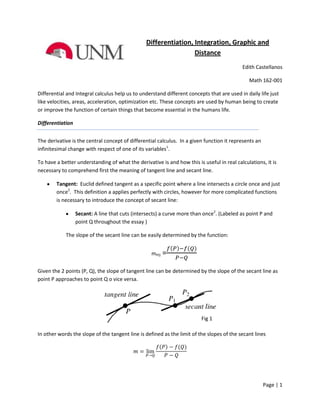
1. Differentiation, Integration, Graphic and
Distance
Edith Castellanos
Math 162-001
Differential and Integral calculus help us to understand different concepts that are used in daily life just
like velocities, areas, acceleration, optimization etc. These concepts are used by human being to create
or improve the function of certain things that become essential in the humans life.
Differentiation
The derivative is the central concept of differential calculus. In a given function it represents an
infinitesimal change with respect of one of its variables1.
To have a better understanding of what the derivative is and how this is useful in real calculations, it is
necessary to comprehend first the meaning of tangent line and secant line.
Tangent: Euclid defined tangent as a specific point where a line intersects a circle once and just
once2. This definition a applies perfectly with circles, however for more complicated functions
is necessary to introduce the concept of secant line:
Secant: A line that cuts (intersects) a curve more than once2. (Labeled as point P and
point Q throughout the essay )
The slope of the secant line can be easily determined by the function:
mPQ =
Given the 2 points (P, Q), the slope of tangent line can be determined by the slope of the secant line as
point P approaches to point Q o vice versa.
Fig 1
In other words the slope of the tangent line is defined as the limit of the slopes of the secant lines
Page | 1

2. An easy way to define the expression for the tangent line is by the substitution of P-Q. Where P-Q can
be consider as H and consequently as P approaches Q it gets closer and closer to zero, so the new limit
can be defined as
The tangent line expression works for every point on a given function, representing those points the
infinitesimal changes with respect of a variable. Just as the definition of the derivative.
With this new relationship we can denote the derivative as:
Being the expression to represent “derivative of
However, finding the derivative by definition is not always simple. Some rules have been developed to
solve the process of differentiation and get the same results. Those rules are applicable if the function is
differentiable.
The derivative of a Constant: It is always zero since the slope it is also zero.
Power Function: A specific pattern is founded by computing several power functions on the
definition.
Constant multiple rule: Even though the derivative of a constant its zero, when the constant is
multiplied by a power function the constant remains. “The derivative of a constant times a
function is the constant times the derivative of the function”2
Sum /Difference rule: The derivative of a sum/difference of functions is the sum /difference of
the derivatives
Page | 2

3. Product Rule: The derivative of a product of two functions is the derivative of the first function
times the second function PLUS the derivative of the second function times the first function
Or
Quotient Rule: The derivative of a quotient is the denominator times the derivative of the
numerator minus the numerator times the derivative of the denominator, all divided by the
square of the denominator.
Or
The differentiation of the trigonometric functions sine and cosine are not easy to determine with the
definition by itself. By the use of limits and other theorems (like the squeeze theorem) the
differentiation of this functions are given as
Functions of the form or composite functions cannot be differentiating using the rules
for simple functions. However there is a special rule named the chain rule that states:
Applications of the derivative:
By definition, the application of the derivative relies on the change with respect a variable.
For example a function of velocity can be described as a change of position with respect of time as well
as acceleration is a change of velocity with respect of time.
And where x (t) is the function of position, v (t) represents the velocity and
a (t) the acceleration.
Another application is to find the maximum and minimum of a function. This is useful in terms of
optimization.
Page | 3

4. Integrals
As derivatives are the central idea in differential calculus, Integrals plays the same role for integral
calculus.
An Integral can be interpreted as a generalization of an area. For specific shapes and lines the area can
easily be determined, however for areas under curved sides is not.
To make a good estimation is useful to sketch a series of rectangles whose area approaches the area
under the curve.
For a better understanding let’s use a graph to explain
On Fig. 2 We can see the approach of the
area under a curve by using rectangles with
Fig 2
equal bases where . The height
of the rectangles is given by a specific point
where each rectangle touches the graph. In
this graph the height is given by
where is a consecutive number
between ( and b= (
We can compute the total area by adding
the areas of the rectangles.
So
Or
Or
(Riemann Sum)
However to get a better approximation is necessary to extend the number of rectangles as much as
possible; being the best approximation we can express the area
under a curve as a sum of infinite number of rectangles.
Using this principle, the definition of a definite integral becomes
Page | 4

5. To take into account all the possibilities of a definite integral (not just when ) the Riemann sum
define the “negative area” by reversing the terms a and b in the integral
(Net Area)
Or if a=b then
Just as the derivatives, integrals also have some properties of integration.
1. Integral of a constant : The integral of a constant is the constant times the length of the definite
interval of integration
2. Integral of a sum/difference: The integral of a sum/difference is the sum/difference of the
integrals
3. Integral of a constant times a function:
Using all the properties above, we can also determine the integrals over intervals.
Antiderivative:
The Antiderivative is defined as the operation that goes backwards from the derivative of a function.
Just as the derivative the antiderivative has a particular pattern. I
In the last example a constant is added, this is because it is not an indefinite integral and the constant fill
all possible solutions of the integral.
Applications:
The integral is useful to find the area under curves. Also to find some sort of volumes by adding the
areas.
Page | 5

6. Graphing
There are some functions that are easy to graph by plotting some points here and there. Even though
this allows us to determine a rough look of a graph we need to plot an exorbitant number of points to
get it and this will turns in a very large amount of work. However by the proper use of some definitions
of calculus we can also get a proper graph and, indeed, a better understanding of the functions.
To get a good graph we can define 4 points to follow.
1. Find the Zeros and/or Asymptotes of the function:The zeros on a function are points where the
function by itself its zero, it is important on the graph because these are points where the graph
touches or crosses the x-axis. On the other hand the asymptotes are points where the function
can get closer and closer but never touches or reaches that particular point, this is important to
understand the behavior of a function in some points.
Or since we consider as the asymptote because is
where the graph is not define.
If the degree of the leading term of the numerator is greater that the degree of the leading term of
the denominator, the function either goes to whatever the case
If the degree of the leading term of the numerator is equal to the degree of the leading term of the
denominator the asymptote becomes the ratio of the coefficients of both leading terms
If the degree of the leading term of the numerator is less than the degree of the leading term of the
denominator the asymptote is simply 0.
2. Find the critical points:The critical points of a function can be described as the points where the
graph reaches it absolute or local max or min values. In other words, the critical points can be
defined as the points where the slope of the tangent line is 0. The last definition gave us a key to
define them mathematically.
3. Find the concavity:If the function has a degree equal or greater than 2 surely have curves that
we can define as concavities. Concavities can be up or down concavities. To find the concavities
we can take the second derivative of the function.
If the concave is down if the concave is down
4. Inflection points: The inflection points are specific points where the concavities of the graph
changes. Is defined as
Considering those for points we can sketch and understand pretty much any graph.
Page | 6

7. Total Distance vs Net Distance
The net distance is considered as a vector, it can be defined as the displacement or how far from the
original position a particle is regardless of the path.
On the other hand the total distance is scalar. It is, in fact, the absolute distance of the particle
regardless of its final position.
Applications:
In calculus we defined as the derivative of the position with respect of time.
In a graph, being the y-axis and in the x-axis, the area under the curve (Integral) is considered as
the distance. However some graphs present negative velocity which in real life can be consider as “going
back” For those kind of graphs we can either determine the total distance and net distance
(displacement)
For example from a point a-c where and can be determined using the properties of
intervals
Total distance
Since is negative the total area is the total displacement
Net distance
or since is negative the final area just
show the distance that the particle moves from the original position.
References
1. Weisstein, Eric W. "Derivative." From MathWorld--A Wolfram Web Resource. http://mathworld.wolfram.com/Derivative.html
2. Stewart, James. Calculus . 7. Toronto: Brooks/Cole, 2012. 45-47. Print.
Graphics
1. Weisstein, Eric W. "Secant Line." From MathWorld--A Wolfram Web Resource. http://mathworld.wolfram.com/SecantLine.html
2. Riemann Sum. N.d. Elementary CalculusWeb. 8 Dec 2012. <http://www.vias.org/calculus/04_integration_01_02.html>.
Page | 7