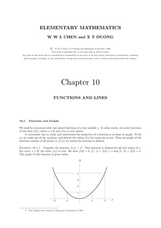
1. ELEMENTARY MATHEMATICS
W W L CHEN and X T DUONG
c W W L Chen, X T Duong and Macquarie University, 1999.
This work is available free, in the hope that it will be useful.
Any part of this work may be reproduced or transmitted in any form or by any means, electronic or mechanical, including
photocopying, recording, or any information storage and retrieval system, with or without permission from the authors.
Chapter 10
FUNCTIONS AND LINES
10.1. Functions and Graphs
We shall be concerned with real valued functions of a real variable x. In other words, we study functions
of the form f (x), where x ∈ R and f (x) is real valued.
A convenient way to study and understand the properties of a function is to draw its graph. To do
so, we make use of the xy-plane, and denote the values f (x) by using the y-axis. Then the graph of the
function consists of all points (x, f (x)) for which the function is defined.
Example 10.1.1. Consider the function f (x) = x2 . This function is defined for all real values of x.
For every x ∈ R, the value f (x) is real. We have f (0) = 0, f (−1) = f (1) = 1 and f (−2) = f (2) = 4.
The graph of this function is given below.
y
4
3
2
1
-2 -1 1 2 x
† This chapter was written at Macquarie University in 1999.

2. 10–2 W W L Chen and X T Duong : Elementary Mathematics
√
Example 10.1.2. Consider the function f (x) = x. This function is defined for all non-negative real
values of x but not defined for any negative√ values of x. For every non-negative x ∈ R, the value f (x)
√
is real. We have f (0) = 0, f (1) = 1, f (2) = 2, f (3) = 3 and f (4) = 2. The graph of this function is
given below.
y
2
1
1 2 3 4 x
10.2. Lines on the Plane
In this section, we shall study the problem of lines and their graphs. Recall first of all that a line is
determined if we know two of its points. Suppose that P (x0 , y0 ) and Q(x1 , y1 ) are two points on the
xy-plane as shown in the picture below.
y
y1 Q(x1 ,y1 )
P(x0,y0)
y0 R(x1,y0)
x
x0 x1
We can consider the triangle P QR formed by P and Q as well as the point R(x1 , y0 ). The length of the
vertical side of this triangle is given by y1 − y0 , while the length of the horizontal side of this triangle is
given by x1 − x0 . The ratio
y1 − y0
x1 − x0
is called the slope of the line through the points P and Q.
Example 10.2.1. The line through the points P (1, 2) and Q(3, 6) has slope
6−2
= 2.
3−1

3. Chapter 10 : Functions and Lines 10–3
Example 10.2.2. The line through the points (4, 0) and (0, 2) has slope
2−0 1
=− .
0−4 2
The line through the points (2, 0) and (0, 1) has slope
1−0 1
=− .
0−2 2
Note that the slope is negative in both cases; see the picture below.
y
2
1
x
1 2 3 4
It is clear that the two lines are parallel to each other. Note that their slopes are equal.
PARALLEL LINES. Two lines on the plane are parallel to each other if and only if their slopes are
equal.
Example 10.2.3. The line through the points (4, 0) and (0, 2) has slope −1/2. It is easy to check that
the line through (1, 0) and (2, 2) has slope 2. We have the following picture.
y
2
1
x
1 2 3 4
-1
-2
It is clear that the two lines are perpendicular to each other. Note that the product of their slopes is
equal to −1.

4. 10–4 W W L Chen and X T Duong : Elementary Mathematics
PERPENDICULAR LINES. Two lines on the plane are perpendicular to each other if and only if
the product of their slopes is equal to −1.
Remark. The two results above are in fact not quite correct. For example, according to our definition,
the line through the points (1, 0) and (1, 1) has slope
1−0 1
=
1−1 0
which is undefined. This represents a vertical line, parallel to the y-axis. On the other hand, a horizontal
line, parallel to the x-axis, has slope 0 (why?). However, in these special cases, we do not need to use
the two results above.
We now consider the problem of finding the equation of the line through two points P (x0 , y0 ) and
Q(x1 , y1 ). Consider the picture below.
y
S (x,y)
Q(x1 ,y1 )
y1
P(x0,y0)
T (x,y0)
y0
R( x1,y0)
x
x0 x1
Suppose that (x, y) is a typical point on the line joining (x0 , y0 ) and (x1 , y1 ). Note that the triangles
P QR and P ST are similar, so that
TS RQ
= .
PT PR
In other words, we must have
y − y0 y1 − y0
= = m,
x − x0 x1 − x0
where
y 1 − y0
m=
x1 − x0
is the slope of the line joining (x0 , y0 ) and (x1 , y1 ). It follows that the equation of the line is given by
y − y0
= m.
x − x0
This can be written in the form
y = mx + c, (1)
where
c = y0 − mx0 .
Note that the y-axis is the line x = 0. If we substitute this into (1), then we ontain y = c. This shows
that the line (1) intersects the y-axis at the point (0, c). This point is called the y-intercept of the line.
On the other hand, the x-intercept of the line is the point of intersection with the x-axis. Note that the
x-axis is the line y = 0. If we substitute this into (1), then we obtain x = −c/m. This shows that the
line (1) intersects the x-axis at the point (−c/m, 0).

5. Chapter 10 : Functions and Lines 10–5
Remark. Again, our argument here fails if the line in question is a vertical line, parallel to the y-axis,
or a horizontal line, parallel to the x-axis.
Example 10.2.4. The line joining the points (1, 0) and (2, 2) is given by
y−0 2−0
= = 2.
x−1 2−1
This can be written in the form y = 2x − 2. Note that this line intersects the y-axis at the point (0, −2)
and the x-axis at the point (1, 0). See the picture in Example 10.2.3.
Example 10.2.5. The line joining the points (1, 1) and (3, 1) is given by
y−1 1−1
= = 0.
x−1 3−1
This can be written in the form y = 1, with m = 0 and c = 1. Note that this line clearly intersects the
y-axis at the point (0, 1) but does not intersect the x-axis. Try to draw the graph of this line.
Example 10.2.6. The line joining the points (1, 1) and (1, 3) is given by x = 1. This is an example of
the exception to our technique. It is easy to see that the line is parallel to the y-axis. It intersects the
x-axis at the point (1, 0) but does not intersect the y-axis. Try to draw the graph of this line.
A line can also be determined if we know its slope and one of its points. Suppose that (x0 , y0 ) is
a given point, and that (x, y) is a typical point on the line through (x0 , y0 ) with slope m. Consider the
following picture.
y
(x ,y)
(x0 ,y0 )
(x,y0)
y0
x
x0
Clearly we must have
y − y0
= m.
x − x0
This again can be rewritten in the form y = mx + c, where c = y0 − mx0 .
Example 10.2.7. The line through the point (1, 2) with slope 3 is given by
y−2
= 3.
x−1
This can be rewritten in the form y = 3x − 1. Note that this line intersects the y-axis at the point
(0, −1) and the x-axis at the point (1/3, 0).

6. 10–6 W W L Chen and X T Duong : Elementary Mathematics
Example 10.2.8. The line y = 4x − 2 has slope 4. We now consider a line parallel to this and passing
through the point (1, 3). This parallel line must also have slope 4, and therefore has equation
y−3
= 4.
x−1
This can be rewritten in the form y = 4x − 1. We consider next a line perpendicular to these two lines
and passing through the point (2, 1). This new line must have slope −1/4, and therefore has equation
y−1 1
=− .
x−2 4
This can be rewritten in the form y = − 1 x + 3 . Try to draw the graphs of these three lines, and find
4 2
their x-intercepts and y-intercepts.
Problems for Chapter 10
1. For each of the following functions, determine the value f (x) for every integer x satisfying the
inequalities −3 ≤ x ≤ 3, and draw a rough sketch of the graph of the function: √
a) f (x) = x2 + 2x − 1 b) f (x) = 4 − x2 c) f (x) = 9 − x2
2. For each of the following, find the equation of the line through the given points:
a) (1, 3) and (2, 5) b) (−1, 3) and (2, 5) c) (−3, 5) and (2, 6)
3. For each of the following, find the equation of the line through the given points, and determine the
x-intercept and y-intercept of this line:
a) (2, 0) and (3, 5) b) (3, −2) and (3, 1) c) (5, −1) and (−1, −1)
4. For each of the following, find the equation of the line with the given slope and passing through the
given point, and determine the x-intercept and y-intercept of this line:
a) slope 3 and point (3, 1) b) slope −2 and point (−1, 4) c) slope 4 and point (4, 2)
5. For each of the three lines in Question 3, find the equation of the perpendicular line which passes
through the point (−4, −4), as well as the intersection of the perpendicular line with the given line.
6. For each of the three lines in Question 4, find the equation of the perpendicular line which passes
through the point (−1, −1), determine its point of intersection with the original line, and then find
the equation of the line which passes through this intersection point and the origin (0, 0).
7. Consider the parabola y = f (x) where f (x) = x2 + 3.
a) Find the slope of the line joining the points (x1 , y1 ) and (x2 , y2 ) on this parabola, where x1 = 1
and x2 = 3.
b) Find the slope of the line joining the points (x3 , y3 ) and (x4 , y4 ) on this parabola, where y3 = 7
and y4 = 19 and where both x3 and x4 are negative.
c) Confirm that the slope of the line in part (a) is equal to x1 + x2 , and that the slope of the line
in part (b) is equal to x3 + x4 .
d) Can you obtain the conclusion of part (c) without using the information about the specific
values of x1 , x2 , y3 and y4 ?
8. Let m1 be the slope of some line, and let m2 be the slope of a perpendicular line. Use trigonometry
to explain why the product m1 m2 is equal to −1, except when one line is horizontal and the other
line is vertical.
− ∗ − ∗ − ∗ − ∗ − ∗ −