Automating Google Workspace (GWS) & more with Apps Script
2012 mdsp pr12 k means mixture of gaussian
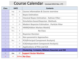
1. Course Calendar (revised 2012 Dec. 27)
Class DATE Contents
1 Sep. 26 Course information & Course overview
2 Oct. 4 Bayes Estimation
3 〃 11 Classical Bayes Estimation - Kalman Filter -
4 〃 18 Simulation-based Bayesian Methods
5 〃 25 Modern Bayesian Estimation :Particle Filter
6 Nov. 1 HMM(Hidden Markov Model)
Nov. 8 No Class
7 〃 15 Bayesian Decision
8 〃 29 Non parametric Approaches
9 Dec. 6 PCA(Principal Component Analysis)
10 〃 13 ICA(Independent Component Analysis)
11 〃 20 Applications of PCA and ICA
12 〃 27 Clustering; k-means, Mixture Gaussian and EM
13 Jan. 17 Support Vector Machine
14 〃 22(Tue) No Class
2. Lecture Plan
Clustering:
K-means, Mixtures of Gaussians and EM
1. Introduction
2. K-means Algorithm
3. Mixtures of Gaussians
4. Re-formation of Mixtures of Gaussians
5. EM algorithm
3. 3
1. Introduction
Unsupervised Learning and Clustering Problem
Given a set of feature vectors without labels of categories, we want to
attempt to find groups or clusters of the data samples in multi-
dimensional space.
We focus the following two methods:
- K-means algorithm
Non-parametric simple technique
- (Gaussian) Mixture models and EM(Expectation Maximization)
/Use a mixture of parametric densities such as Gaussians.
/The optimal model parameters are not given in a closed form
because of a highly non-linear coupled equations.
/The expectation-maximization algorithm is effective for
determining the optimal parameters.
4. 4
1 2
:D-dimensional random vector
N dataset of : X:={ , , , }
: A group of data points whose inter-distances are small
compared with the distances to the points outside of the cluster
N
Cluster
Prototy
x
x x x x
of cluster: 1
: Find a set of vectors , such that the sum of the squared
disstances of each point to its cvlosest vector is minimized.
k
k
k
k K
K
pe
Aim
2. K-means Algorithm
The K-means algorithm is a non-statistical approach of clustering of
data points in multi-dimensional feature space.
Problem: Partition the dataset into some number K of clusters
(K is known)
Fig. 1
1 [Bishop book[1] and its web site]
6. 6
-Assignment indicator
1 if is assigned to -th cluster
0
n
nk
k
r
otherwise
x
Algorithm
Introduce variable rnk denoting the assignment of data point
2
1 1
-Object Function (Distortion measure)
N K
nk n k
n k
J r
x
Squared of distance of each point xn to
its assigned vector 𝝁k
-Find both and which minimizenk kr J
(1)
(2)
7. 7
(0)
( )
- : for the
- : Minize J with respect to for fixed
- : Minimize J with respect to for fixed
k k
i
nk
k nk
r
r
Two - stage Optimization
initial value
First stage
Second stage
:
Determination of for given 1~ at
at argmin1
0
That is, we assign the to the closest cluster center.
nk k n
n j
j
nk
n
r k K x
k x
r
otherwise
x
First stage
(3)
8. 8
:
Optimization of
0 2 0
Above equation gives the mean vector of all data points
assinged to cluster .
k
nk n k
nk
nk nn
k
nkn
n
J
r x
r x
r
x
k
Second stage
the number of points assigned
to cluster k
the sum of xn which assigned to
cluster k
(4)
10. Fig. 3 [1]
Application of k-means algorithm for color-based image
segmentation [Bishop book[1] and its web site]
K-means clustering applied to the color vectors of pixels in RGB
color-space
11. 11
1
[Mixture of Gaussians]
Conside a superposition of Gaussians (Normal distributions)
,
K
k k k
k
K
p x x
3. Mixtures of Gaussians
- Limitations of single Gaussian pdf model
Examples [Bishop[1]]
Single Gaussian model does not capture the multi-modes feature.
Fig 4
Mixture distribution approach: uses the linear combination of basic
distributions such as Gaussians
mixing coefficients mixture component
(5)
single Gaussian Mixture of Gaussians
13. 13
1
1 1
0 0 1
The ( 1 ) satisfy the discrete probability requirements.
:The prior probability of selecting the -mixture component
,
K
k
k
k
k
k
k k
p x dx
p x
k K
p k k
x p x
1
responsibilit
: The probability of
i
with condition on
From Eq. (5)
- Define the by the posterior distributioe n
:
,
=
s
,
K
k
k
k
k k k
l l l
x k
p x p k p x k
x p k x
x p k x
p k p x k x
p x
x
1
K
l
(7)
(6)
14. 14
1 2
1 2
1 2
1 2
(*)
(* see lect
- Parameters of mixture Gaussian (5)
:= , , ,
:= , , ,
:= , , ,
- Observed data X:= , , , Estimatte , ,
- Apply Maximum Likelihood method
K
K
K
Nx x x
1 1
ure 2 slides for a single Gaussian distribution case)
- Maximize the Log-Likelihood function
ln , , ln ,
N K
k n k k
n k
p X N x
Too complex to give closed form solution
Go to EM (Expectation Maximization) algorithm
(8)
15. 15
4. Re-formation of Mixtures of Gaussians
Formulation of Mixture of Gaussians in terms of discrete latent random
variables
- Introduce K-dimensional random variable z
- 1-of-K representation model of πk
1 2
1
: , , ,
0,1 and 1
1
T
K
K
k k
k
k k
z z z
z z
p z
z
ln , ,
z
p x p z p x z p X
Equivalent formulation of the Gaussian mixture with explicit
latent variable z
(9)
16. 16
1 1
- The conditional probability of for given
: 1
1 1 ,
1 1 ,
k k
k k k k k
K K
k k j j j
j j
z x
z p z x
p z p x z N x
p z p x z N x
The responsibility that component k
takes for explaining the observation x
The posterior probability for observed x
The prior probability of zk=1
1 2
1
- Modeling a data set X:= , , , using a mixture of Gaussians
Assuming , , are drawn independently from , ,
the Log-Likelihood function is given by Eq.()
N
N k k
x x x
x x p x
(10)
17. 17
- With respect to and , the conditions that must be
satisfied at a maximum of the likelihood function
k k
1 1
- Maximization of ln , , with respect to
subject to a constraint 1 is also solved.
- Solutions are given by
1
where :
k
kk
N N
k nk n k nk
n nk
k
p X
z x N z
N
1
The responsibility of with respect to -th cluster
1
where =Eq. (10) n
N
T
nk n k n k
nk
k
k
nk x k
z x x
N
N
N
z
5. EM Algorithm
ln , ,
0, ,k k
p X
(11)
(14)
(13)
(12)
18. 18
Three equations ()-() do not give solutions directly because
, contain unknowns , , and in complex ways.
[EM algorithm for Gaussian Mixture Mode]
Simple iterative scheme which altaernate the
nk kz N
E (Expectation)
and M (Maximization) steps.
: Evaluate the posterior probabilities (responsibilities)
using the current parameters
: Re-estimate parameters , , a
nkz
E step
M step
nd using the
evaluated
Color illustration of in two-category case
nk
nk
z
z
22. 22
References:
[1] C. M. Bishop, “Pattern Recognition and Machine Learning”,
Springer, 2006
[2] R.O. Duda, P.E. Hart, and D. G. Stork, “Pattern Classification”,
John Wiley & Sons, 2nd edition, 2004
23. 23
2
1 1
21
1
2
2 2
2
Proof of 1-dimensional case
ln , , ln ,
ln , , 0
,
- When
1
,
derives Eq.
,
,
1( 2)
n k k
n k k
N K
j n j j
n j
kN
K
n
j n j j
j
k
n k k n k
k k
N x
N x
p X N x
p X
N x
N x x
Appendix
(A.1)
(A.2)
(A.3)
24. 24
22
1
2
- When
Calculate and substitute it into Eq. (A.2)
derives
1
,
k
N
k nk n k
n
k
k
n
k
k
z x
N x
N
For the maximization problem of ln , , with respect
to subject to 1 , Lagrange multiplier method provides
an elegant solution.
- Introduce Lagragian function given by
, : ln ,
k kk
k
p X
L p X
, 1kk
(A.4)
(A.5)
25. 25
2
21
1
2
21
1
- Stationarity conditions
, ,
0, 0
,,
0
,
Multiply both sides above, we have
,
,
, and the s
k k
k
N
n k kk
K
nk
j n j j
j
k
N
k n k k
kK
n
j n j j
j
L L
N xL
N x
N x
N x
2
21
1
ummation over gives
,
,
N
k n k kk
kK k
n
j n j j
j
k
N x
N x
(A.6)
(A.7)
(A.8)
26. 26
2
21
1
We then have
From (A.7),
,1
=
,
N
k n k k k
k K
n
j n j j
j
N
N x N
N N
N x
(A.9)