This document describes a damped oscillation graph of a spring-mass system experiencing dry frictional force. The system performs damped harmonic oscillation as the mass oscillates back and forth along the horizontal surface. The document provides the equation of motion, solution, and a Maple code to plot the decreasing amplitude oscillation graph over multiple periods as a function of time.
1. Graph of COULOMB-DRY-FRICTION DAMPED OSCILLATION
In MAPLE, people often use the seq function to create the list.
However, to make switching from maple to javascript and to latex easily, I try to use for..do to create
aray ARR, after that convert aray into list by using function
convert (ARR, list)
1. Problem:
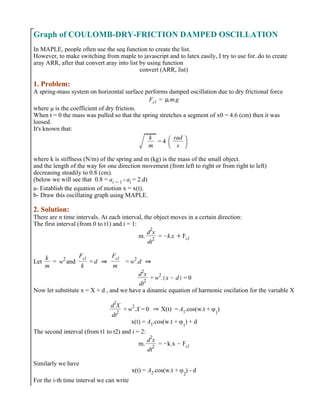
A spring-mass system on horizontal surface performs damped oscillation due to dry frictional force
Fcl = µ.m.g
where µ is the coefficient of dry friction.
When t = 0 the mass was pulled so that the spring stretches a segment of x0 = 4.6 (cm) then it was
loosed.
It's known that:
k
m
= 4
rad
s
where k is stiffness (N/m) of the spring and m (kg) is the mass of the small object.
and the length of the way for one direction movement (from left to right or from right to left)
decreasing steadily to 0.8 (cm).
(below we will see that 0.8 = ai K1 - ai = 2.d)
a- Establish the equation of motion x = x(t).
b- Draw this oscillating graph using MAPLE.
2. Solution:
There are n time intervals. At each interval, the object moves in a certain direction:
The first interval (from 0 to t1) and i = 1:
m.
d
2
x
dt
2
= Kk.x CFcl
Let
k
m
= w
2
and
Fcl
k
= d 0
Fcl
m
= w
2
.d 0
d
2
x
dt
2
+ w
2
. x Kd = 0
Now let substitute x = X + d , and we have a dinamic equation of harmonic oscilation for the variable X
d2
X
dt
2
+ w
2
.X = 0 0 X(t) = A1.cos(w.t + 4
1
)
x(t) = A1.cos(w.t + 4
1
) + d
The second interval (from t1 to t2) and i = 2:
m.
d
2
x
dt
2
= Kk.x KFcl
Similarly we have
x(t) = A2.cos(w.t + 42
) - d
For the i-th time interval we can write
2. x(t) = Ai.cos(w.t + 4
i
) + K1
i K1
.d (a)
From the initial conditions for the first interval (when t=0 x = x0 and v =
d
d t
x = 0) we can get
4
1
= 0 (if x0>0) ; 4
1
= π (if x0<0) (b)
a- We can show that all phases are equal to 4
1
The function x (t) is a continuous and, at the moment t1 when the mass changes the direction of its
motion, function xi K1 "changes" to xi, so at this moment we have:
xi = xi K1 ; vi = vi K1 = 0
0 - w.Ai.sin w.ti C 4
i
= 0 0 w.ti C 4
i
= p.π p = 0, 1, 2, 3 ...
- w.Ai K1.sin w.ti C 4
i K1
= 0 0 w.ti C 4
i K1
= q.π q = 0, 1, 2, 3 ...
Because 0 ≤ 4
i
! 2 π we have
4
i
- 4
i K1
= 0 OR π 1
However from xi = xi K1 we have
cos(w.ti C 4
i
= cos w.ti C 4
i K1
2
In (2) we can't substitute 4
i
= 4
i K1
C π. So we have
4i
= 4i K1
= 41
3
a- We can show that the amplitude of sinusoidal (harmonic) oscilation (in the interval from ti K 1
to ti is
Ai = x0 K 2. i K 1 C 1 .d
We will call a0 = x0 , a1 , a2 , a3 ... the amplitudes of damped oscillation. We have :
2. Ai = ai K1 C ai 4
According to the work-energy theorem we have:
1
2
.k.ai
2
=
1
2
.k.ai K1
2
KFcl. ai K1 C ai 0 ai = ai K1 K2. d 5
By subtituting (5) to (4) we have
Ai = ai K1 Kd 6 0 Ai K1 = ai K2 Kd 7
From (5),(6),(7) we get
Ai = Ai K1 K2. d 7
So, according to (6)
A1 = a0 Kd = x0 Kd
According to (7)
A2 = x0 Kd K2 d = x0 K 3 d
0 Ai = x0 K 2. iK1 C 1 .d i = 1, 2, 3 ... 8
With MAPLE we have to write : if a0 is the amplitude at t = 0
a0 := abs(x0);
If x0 > 0 then the equation of motion for the i-th half period is:
x(t) = (a0 - (2*(i-1) + 1)*d)*cos(w*t) + (-1)^(i-1)*d; (i = 1,2,3...)
3. >>
(1)(1)
>>
>>
>>
(2)(2)
>>
>>
>>
If x0 < 0 then the equation of motion for the i-th half period is:
x(t) = (a0- (2*(i-1) + 1)*d)*cos(w*t + Pi) - (-1)^(i-1)*d; (i = 1,2,3...)
ai is the amplitude at the end of i-th half-period.
ai = a0 - (2*d)*i; (i = 1,2,3 ...)
If ai ≤ d then ai ≤
Fcl
k
0 k$ai ≤ Fcl 0 the mass stops
i ≥ (a0 - d)/(2*d)
DEFINITION: The ceiling of a real number x is defined to be the smallest integer no smaller than x.
So the number of half-period is
n = ceil((a0-d)/(2*d)) (9)
# Please correct the data of
# x0 (cm) (x0>0 or x0<0) , w (rad/s), d (cm) as you want
# then click the button with three exclamation points (!!!):
x0:=4.6; w:=4; d:=0.4;
# You need not to change the value of xtext
xtext:= 0.2:
a0 := abs(x0);
x0 d 4.6
w d 4
d d 0.4
a0 d 4.6
with(plots):
n := ceil((a0-d)/(2*d));
T:= 2*Pi/w:
tt := n*1/2*T:
tt1 := 1/100*round(tt*100):
tt2 := parse(sprintf("%.2f",tt1)):
print(`Total time of motion: `,tt,` = `, tt2,` (sec)`);
n d 6
Total time of motion: ,
3 π
2
, = , 4.71, (sec)
P:= Array(1..n):
for i from 1 to n do
if x0 > 0 then
P[i] := plot((a0 - (2*(i-1) + 1)*d)*cos(w*t) + (-1)^(i-1)*d, t=
(i-1)*Pi/w..i*Pi/w,thickness=1,color=blue);
else
P[i] := plot((a0 - (2*(i-1) + 1)*d)*cos(w*t + Pi) - (-1)^(i-1)*d,
t= (i-1)*Pi/w..i*Pi/w,thickness=1,color=blue);
end if;
end do:
pic:= convert(P,list):
B:= Array(1..n+1):
for i from 1 to n+1 do
b:= (a0 - (2*d)*i)*sign(x0);
5. t
π
4
π
2
3 π
4
π 5 π
4
3 π
2
K3
K2
K1
0
1
2
3
4
In MAPLE 16, we can export the graph as PDF image:
- Right click the graph.
- Select Export then select Portable Document Format
6. >>
>>
>>
>>
>>
>>
>>
>>
>>
>>
>>
>>
>>
>>
Here is the mpl file. You can select it all , copy , paste the content to Notepad , delete the green
simbol # placed at the beginning of lines and save as coulomb-graph.mpl.
After that you can open this file in MAPLE.
# # Please correct the data of
# # x0 (cm) (x0>0 or x0<0) , w (rad/s), d (cm) as you want
# # then click the button with three exclamation points (!!!):
# x0:=4.6; w:=4; d:=0.4;
# # You need not to change the value of xtext
# xtext:= 0.2:
# a0 := abs(x0);
# with(plots):
# n := ceil((a0-d)/(2*d));
# T:= 2*Pi/w:
# tt := n*1/2*T:
# tt1 := 1/100*round(tt*100):
# tt2 := parse(sprintf("%.2f",tt1)):
# print(`Total time of motion: `,tt,` = `, tt2,` (sec)`);
7. >>
>>
>>
>>
>>
>>
>>
>>
>>
>>
>>
>>
>>
>>
>>
>>
>>
>>
>>
>>
>>
>>
>>
>>
>>
>>
# P:= Array(1..n):
# for i from 1 to n do
# if x0 > 0 then
# P[i] := plot((a0 - (2*(i-1) + 1)*d)*cos(w*t) + (-1)^(i-1)*d, t=
(i-1)*Pi/w..i* Pi/w,thickness=1,color=blue);
# else
# P[i] := plot((a0 - (2*(i-1) + 1)*d)*cos(w*t + Pi) - (-1)^(i-1)*
d, t= (i-1)*Pi/w..i*Pi/w,thickness=1,color=blue);
# end if;
# end do:
# pic:= convert(P,list):
# B:= Array(1..n+1):
# for i from 1 to n+1 do
# b:= (a0 - (2*d)*i)*sign(x0);
# L:=[[i*Pi/w,0],[i*Pi/w,(-1)^i*b]];
# B[i] := plot(L,t=0..4,thickness=0,color=green);
# end do:
# amp:= convert(B,list):
# T0:=textplot([xtext,sign(x0)*a0/2,'a0']):
# T1:= textplot([Pi/w + xtext,sign(x0)*(-1)*(a0-2*d)/2,'a1']):
# T2:= textplot([2*Pi/w + xtext,sign(x0)*(a0-4*d)/2,'a2']):
# tex := [T0,T1,T2]:
# LA:=[[0,d],[(n+1)*Pi/w,d]]:
# linA:=plot(LA,t=0..4,thickness=0,color=red):
# LB:=[[0,-1*d],[(n+1)*Pi/w,-1*d]]:
# linB:=plot(LB,t=0..4,thickness=0,color=red):
# lin := [linA, linB]:
# display(pic,amp,tex,lin);
# display(pic,lin);
3. We can also draw this graph using this html file
<!DOCTYPE HTML>
<html>
<head>
<meta http-equiv="content-type" content="text/html; charset=utf-8">
<title>Coulomb OSC</title>
<head>
<style>
body{
font-family:'Arial';
font-size:11pt;
margin:0px; padding:0px;
background-color:#99CCFF;
}
input[type=text]{background-color:white; text-align:center}
button{background-color:#DDDDDD}
</style>
<link rel="stylesheet" type="text/css" href="http://jsxgraph.uni-bayreuth.de/distrib/jsxgraph.css"
9. var brd1 = JXG.JSXGraph.initBoard('box', {boundingbox: [0, 13, wid, -13], axis:true});
function show(){
w = Number(document.getElementById('omega').value);
x0 = Number(document.getElementById('x0').value);
d = Number(document.getElementById('d').value);
n = Math.ceil((x0 - d)/(2*d));
for(i= 1; i<= n; i++){
mm1 = x0-(2*(i-1)+1)*d + d;
mm = Math.round(mm1 * 100) / 100;
if(i % 2 == 1){mm ='<span style="color:red">'+ mm + '</span>'}
if((i+1) % 10 == 0 ){mm = mm + '<br>'}
st = document.getElementById('div1').innerHTML;
document.getElementById('div1').innerHTML = st + ' ; ' + mm;
f = brd1.createElement('functiongraph',
[function(x){
if(x>(i-1)*Pi/w && x <i*Pi/w){
011 return (x0-(2*(i-1)+1)*d)*Math.cos(w*x) + Math.pow(-1,i-1)*d;
}else{
return 0
// break;
}
}]);
}
mm2 = (x0-(2*n+1)*d)*Math.cos(Pi*(n+2)) + Math.pow(-1,n)*d;
mm3 = Math.round(mm2 * 100) / 100;
st = document.getElementById('div1').innerHTML;
document.getElementById('div1').innerHTML = st +
'<br><span style="color:green"><b>Stop at: ' + mm3+'</b></span>';
var xr = brd1.create('line',[[0,0],[10,0]],{visible:true, strokeColor: "#CCCCCC"});
}
function saveSVG(){
var svg = new XMLSerializer().serializeToString(brd1.renderer.svgRoot);
// alert(svg);
var blob = new Blob([svg], {type: "text/plain;charset=utf-8"});
saveAs(blob, "cl-damped-1.svg");
}
function clr(){
brd1 = JXG.JSXGraph.initBoard('box', {boundingbox: [0, 13, wid, -13], axis:true});
document.getElementById('div1').innerHTML = '';
}
</script>
</body>
</html>
10. 4. Latex code and using overleaf.com for compiling from tex to pdf
documentclass[crop,tikz]{standalone}
usepackage[utf8]{vietnam}
usepackage[utf8]{inputenc}
usepackage{amsmath,amsxtra,amssymb,amsthm,latexsy m,amscd,amsfonts}
usepackage{pgfplots}
usepackage{tikz}
usepackage{tkz-tab}
usepackage{graphics}
usepackage{fp}
begin{document}
newcommand{ww}{4}
11. newcommand{posit}{1}
newcommand{xx}{4.6}
newcommand{dd}{0.4}
newcommand{negat}{(-1)*xx}
begin{tikzpicture}small
begin{axis}[trig format plots=rad, axis line style=gray,
samples=120,
width=12.0cm,height=9.0cm,
xmin=0, xmax=2*pi,
ymin=-6, ymax=6,
axis x line=center,
axis y line=center,
xlabel=$t$,ylabel=$x$]
pgfmathparse{ceil((xx - dd)/(2*dd))}edefstoreresult{pgfmathresult}
FPeval{nn}{storeresult};
foreach i in {1,...,nn} {
ifnumposit = 0{
addplot[red,domain=(i-1)*pi/ww:(i)*pi/ww,semithick]
{(abs(xx) -(2*i-1)*dd)*cos(ww*x + pi) - ((-1)^(i-1))*dd};
}
else{
addplot[blue,domain=(i-1)*pi/ww:(i)*pi/ww,semithick]
{((xx-(2*i-1)*dd)*cos(ww*x) + ((-1)^(i-1))*dd)};
}
fi
}
end{axis}
end{tikzpicture}
end{document}
12. 4- Remark
In fact, we only provide an algorithm for the case
|x0| = N.2d + δ where δ ≤ d ; N = 1, 2, 3 ...
However, the above algorithm is still valid for the case
|x0| = N.2d + d + δ (In this case the mass does not pass the x = 0 point).