Master of Computer Application (MCA) – Semester 4 MC0079-Computer based Optimization Methods

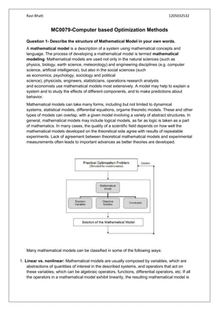
1. Ravi Bhatt 1205032532
MC0079-Computer based Optimization Methods
Question 1- Describe the structure of Mathematical Model in your own words.
A mathematical model is a description of a system using mathematical concepts and
language. The process of developing a mathematical model is termed mathematical
modeling. Mathematical models are used not only in the natural sciences (such as
physics, biology, earth science, meteorology) and engineering disciplines (e.g. computer
science, artificial intelligence), but also in the social sciences (such
as economics, psychology, sociology and political
science); physicists, engineers, statisticians, operations research analysts
and economists use mathematical models most extensively. A model may help to explain a
system and to study the effects of different components, and to make predictions about
behavior.
Mathematical models can take many forms, including but not limited to dynamical
systems, statistical models, differential equations, orgame theoretic models. These and other
types of models can overlap, with a given model involving a variety of abstract structures. In
general, mathematical models may include logical models, as far as logic is taken as a part
of mathematics. In many cases, the quality of a scientific field depends on how well the
mathematical models developed on the theoretical side agree with results of repeatable
experiments. Lack of agreement between theoretical mathematical models and experimental
measurements often leads to important advances as better theories are developed.
Many mathematical models can be classified in some of the following ways:
1. Linear vs. nonlinear: Mathematical models are usually composed by variables, which are
abstractions of quantities of interest in the described systems, and operators that act on
these variables, which can be algebraic operators, functions, differential operators, etc. If all
the operators in a mathematical model exhibit linearity, the resulting mathematical model is

2. Ravi Bhatt 1205032532
defined as linear. A model is considered to be nonlinear otherwise. The question of linearity
and nonlinearity is dependent on context, and linear models may have nonlinear expressions
in them. For example, in a statistical linear model, it is assumed that a relationship is linear in
the parameters, but it may be nonlinear in the predictor variables. Similarly, a differential
equation is said to be linear if it can be written with linear differential operators, but it can still
have nonlinear expressions in it. In a mathematical programming model, if the objective
functions and constraints are represented entirely by linear equations, then the model is
regarded as a linear model. If one or more of the objective functions or constraints are
represented with a nonlinear equation, then the model is known as a nonlinear model.
Nonlinearity, even in fairly simple systems, is often associated with phenomena such as
chaos and irreversibility. Although there are exceptions, nonlinear systems and models tend
to be more difficult to study than linear ones.
2. Deterministic vs. probabilistic (stochastic): A deterministic model is one in which every set
of variable states is uniquely determined by parameters in the model and by sets of previous
states of these variables. Therefore, deterministic models perform the same way for a given
set of initial conditions. Conversely, in a stochastic model, randomness is present, and
variable states are not described by unique values, but rather by probability distributions.
3. Static vs. dynamic: A static model does not account for the element of time, while a dynamic
model does. Dynamic models typically are represented with difference equations or
differential equations.
4. Discrete vs. Continuous: A discrete model does not take into account the function of time
and usually uses time-advance methods, while a Continuous model does. Continuous
models typically are represented with f(t) and the changes are reflected over continuous time
intervals.
5. Deductive, inductive, or floating: A deductive model is a logical structure based on a
theory. An inductive model arises from empirical findings and generalization from them. The
floating model rests on neither theory nor observation, but is merely the invocation of
expected structure. Application of mathematics in social sciences outside of economics has
been criticized for unfounded models. Application of catastrophe theory in science has been
characterized as a floating model.
Question 2 - Explain Erlang family of distributions of service times.
The Erlang distribution is a continuous probability distribution with wide applicability
primarily due to its relation to the exponential and Gamma distributions. The Erlang
distribution was developed by A. K. Erlang to examine the number of telephone calls which
might be made at the same time to the operators of the switching stations. This work on
telephone traffic engineering has been expanded to consider waiting times in queuing
systems in general. The distribution is now used in the fields of stochastic processes and
of biomathematics.
Probability density function
The probability density function of the Erlang distribution is

3. Ravi Bhatt 1205032532
The parameter is called the shape parameter and the parameter is called the rate
parameter. An alternative, but equivalent, parameterizations (gamma distribution) uses the
scale parameter which is the reciprocal of the rate parameter (i.e., ):
When the scale parameter equals 2, the distribution simplifies to the chi-squared
distribution with 2k degrees of freedom. It can therefore be regarded as a generalized chi-
squared distribution, for even degrees of freedom.
Because of the factorial function in the denominator, the Erlang distribution is only defined
when the parameter k is a positive integer. In fact, this distribution is sometimes called the
Erlang-k distribution (e.g., an Erlang-2 distribution is an Erlang distribution with k=2). The
Gamma distribution generalizes the Erlang by allowing to be any real number, using the
gamma function instead of the factorial function.
Cumulative distribution function (CDF)
The cumulative distribution function of the Erlang distribution is:
where is the lower incomplete gamma function. The CDF may also be
expressed as
Question 3 - Explain the algorithm for solving a linear programming problem by graphical
method.
Linear programming (LP) is a mathematical method for determining a way to achieve the
best outcome (such as maximum profit or lowest cost) in a given mathematical model for
some list of requirements represented as linear equations. More formally, linear
programming is a technique for the optimization of a linear objective function, subject to
linear equality and linear inequality constraints. Given a polytope and a real-valued affine
function defined on this polytope, a linear programming method will find a point on the
polytope where this function has the smallest (or largest) value if such point exists, by
searching through the polytope vertices.
An Algorithm for solving a linear programming problem by Graphical Method:(This algorithm
can be applied only for problems with two variables).
Step – I: Formulate the linear programming problem with two variables (if the given problem
has more than two variables, then we cannot solve it by graphical method).
Step – II: Consider a given inequality. Suppose it is in the form a1x1 + a2x2 <= b (or a1x1 +
a2x2 >= b). Then consider the relation a1x1+ a2x2= b. Find two distinct points (k, l), (c, d)
that lie on the straight line a1x1+ a2x2= b. This can be found easily: If x1= 0, then x2 = b /

4. Ravi Bhatt 1205032532
a2.If x2=0, then x1 = b / a1. Therefore (k, l) = (0, b / a2) and (c, d) = (b / a1, 0) are two points
on the straight line a1x1+a2x2= b.
Step – III: Represent these two points (k, l), (c, d) on the graph which denotes X–Y-axis
plane. Join these two points and extend this line to get the straight line which represents
a1x1+ a2x2= b.
Step – IV: a1x1 + a2x2= b divides the whole plane into two half planes, which are a1x1+
a2x2 <= b (one side) and a1x1+ a2x2 >= b (another side). Find the half plane that is related
to the given inequality.
Step – V: Do step-II to step-IV for all the inequalities given in the problem. The intersection of
the half-planes related to all the inequalities and x1 >= 0,x2 >= 0 , is called the feasible
region (or feasible solution space). Now find this feasible region.
Step – VI: The feasible region is a multisided figure with corner points A, B,C, … (say). Find
the co-ordinates for all these corner points. These corner points are called as extreme
points.
Step – VII: Find the values of the objective function at all these corner/extreme points.
Step – VIII: If the problem is a maximization (minimization) problem, then the maximum
(minimum) value of z among the values of z at the corner/extreme points of the feasible
region is the optimal value of z. If the optimal value exists at the corner/extreme point, say A
(u, v), then we say that the solution x1= u and x2= v is an optimal feasible solution.
Step – IX:Write the conclusion (that include the optimum value of z, and the co-ordinates of
the corner point at which the optimum value of z exists).
Question 4 - Determine optimal solution to the problem given below. Obtain the initial
solution by VAM. Write down the differences between PERT and CPM.
Warehouses Stores Availability
I II III IV
A 5 1 3 3 34
B 3 3 5 4 15
C 6 4 4 3 12
D 4 -1 4 2 19
Requirement 21 25 17 17 80
Since the aggregate supply is 220 units and the aggregate demand is 200 units, we shall
introduce a dummy market, M5, for an amount equal to 20 (the difference between the
aggregate supply and demand), with all cost elements equal to zero. The solution is given in
a one table. The initial solution obtained by VAM is degenerate, since it contains only seven
basic variables (since there are only 7 cells occupied and not 8 (= 4 + 5 -1) required for non-
degeneracy).

5. Ravi Bhatt 1205032532
Here empty cells P1M3, P2M3, P3M1, P3M2, P3M4, P3M5, and P4M3 are independent
while others are not.
For removing degeneracy place in the cell P3M5and then test it for optimality. This is
done in the following table.
This solution is found to be non-optimal.
Therefore the total cost is:
Rs. (6 x 30) + (1 x 10) + (3 x 20) + (0 x 50) + (7 x 60) + (1 x 30) = 700.
CPM was developed by Du Pont and the emphasis was on the trade-off between the
cost of the project and its overall completion time (e.g. for certain activities it may be possible
to decrease their completion times by spending more money - how does this affect the
overall completion time of the project?)
Definition: In CPM activities are shown as a network of precedence relationships using
activity-on-node network construction
– Single estimate of activity time
– Deterministic activity times
USED IN: Production management - for the jobs of repetitive in nature where the
activity time estimates can be predicted with considerable certainty due to the existence of
past experience.
PERT was developed by the US Navy for the planning and control of the Polaris
missile program and the emphasis was on completing the program in the shortest possible
time. In addition PERT had the ability to cope with uncertain activity completion times (e.g.
for a particular activity the most likely completion time is 4 weeks but it could be anywhere
between 3 weeks and 8 weeks).
Basic difference between PERT and CPM:
Though there are no essential differences between PERT and CPM as both of them
share in common the determination of a critical path and are based on the network
representation of activities and their scheduling that determines the most critical activities to
be controlled so as to meet the completion date of the project.
PERT:
1. Since PERT was developed in connection with an R and D work, therefore it had to
cope with the uncertainties which are associated with R and D activities. In PERT,
total project duration is regarded as a random variable and therefore associated
probabilities are calculated so as to characterize it.

6. Ravi Bhatt 1205032532
2. It is an event-oriented network because in the analysis of network emphasis is given
an important stages of completion of task rather than the activities required to be
performed to reach to a particular event or task.
3. PERT is normally used for projects involving activities of non-repetitive nature in which
time estimates are uncertain.
4. It helps in pinpointing critical areas in a project so that necessary adjustment can be
made to meet the scheduled completion date of the project.
CPM:
1. Since CPM was developed in connection with a construction project which consisted
of routine tasks whose resources requirement and duration was known with certainty,
therefore it is basically deterministic.
2. CPM is suitable for establishing a trade-off for optimum balancing between schedule
time and cost of the project.
3. CPM is used for projects involving activities of repetitive nature.
Project scheduling by PERT-CPM:
It consists of three basic phases: planning, scheduling and controlling.
1. Project Planning.
2. Scheduling.
3. Project Control.
Question 5 - Explain the use of finite queuing tables.
There will be cases, where the possible number of arrivals is limited and is relatively small.
In a production shop, if the machines are considered as customers requiring service from
repair crews or operators, the population is restricted to the total number of machines in the
shop. In a hospital ward, the probability of the doctors or nurses being called for service is
governed by the number of beds in the ward. Similarly, in an aircraft the number of seats is
finite and the number of stewardesses provided by the airlines will be based on the
consideration of the maximum number of passengers who can demand service. As in the
case of a queuing system with infinite population, the efficiency of the system can be
improved in tens of reducing the average length of queues, average waiting time and time
spent by the customer in the system by increasing the number of service channels.
However, such increases mean additional cost and will have to be balanced with the benefits
likely to accrue. If the queuing system in a machine shop is under study, the cost of
providing additional maintenance crews or operators can be compared with the value of
additional production possible due to reduced downtime of the machines` In cases where it
is not possible to quantify the benefits, the management will have to base its decisions on
the desired standards for customer service
The queue discipline in a finite queuing process can be:
i) First come-first served
ii) Priority e.g.: Machines of high cost may be given priority for maintenance while
others may be kept waiting even if they had broken down before.

7. Ravi Bhatt 1205032532
iii) Random e.g.; in a machine shop if a single operator is attending to several
machines and several machines call for his attention at a time, he may attend first
to the one nearest to him.
The analysis of Finite Queuing Models is more complex than those with infinite population
although the approach is similar.
Notations: Notations used are different and are given below:
N - Population (machines, customers etc)
M - Service channels (repairmen, telephone lines etc.)
T - Average service time (repair time length of conversation on a telephone etc.)
W - Average waiting time
U - Average running time (of machines) or mean time between calls for service per unit H -
Average number of units being serviced
L - Average number of units waiting for service
J - Average number of units in operation
X - Service Factor
Probability that if a unit calls for service, it will have to wait,
Let us consider a machine shop with N machines. The inter breakdown time of these
machines follows a negative
l exponential distribution with mean U. The number of breakdowns follows Poisson
distribution with mean À. It is assumed that machines are kept running (or in operation)
except when they are under repairs or waiting for repair crew to attend. If M repair crews are
available, the time taken by any crew follows a negative exponential distribution with mean
T. Naturally a machine which has broken down will have to wait for repairs if all the repair
crews are busy.
The tables give the values of F and D for different values of N, M and X. They are arranged
in the ascending order of the values of the population. For each N, the value of X increases
from .001 to .950. For a given service factor X, several values of M can be found. For each
value of X and M, values of D and F are tabulated,
The steps in the use of Finite Queuing Tables may be summarized as follows'.
(i) Find mean service timeTand mean running tirne U.
(ii) Compute the service factor
(iii) Select the table corresponding to the population N.
(iv) For the given population, locate the service factor value.
(v) Read off from tables, values of D and F for the number of service crews M.
If necessary, these values may be interpolated between relevant values of X. (vi) Calculate
the other measures L W, H, and J from the formulae given.
The overall efficiency F of the system will increase with the number of service channels (M)
provided. As mentioned earlier, addition of service crews involves cost, which should be
justified by the increase in the efficiency of the system i.e. additional running time of

8. Ravi Bhatt 1205032532
machines possible. However it will be seen from the tables that as M increase the rate 0f
increase in efficiency decreases. The practical significance is that beyond a certain value of
M, it is not worthwhile increasing M as there would be no appreciable increase in the
efficiency of the system.
Questions 6 - Customers arrive at a small post office at the rate of 30 per hour.
Service by the clerk on duty takes an average of 1 minute per customer
a) Calculate the mean customer time.
(i) Spent waiting in line
(ii) Spent receiving or waiting for service.
b) Find the mean number of persons
(i) in line
(ii) Receiving or waiting for service.
Mean arrival rate λ = 30 customers per hour = ½ customer per minute.
Mean service rate λ = 1 per minute
Traffic intensity
P = λ/µ
= ½
a) Mean Customer Time
a. Spent waiting in line
E(w) = λ/( µ(µ - λ))
= 1 minute
b. Spent receiving or waiting for service
W(v) = 1/( µ - λ)
= 2 minutes
b) Find the mean number of persons
a. in line
E(m) = λ2
/( µ(µ - λ))
= ½ Customer
b. Receiving or waiting for service
E(n) = λ /( µ - λ)
= 1 Customer