most important notes

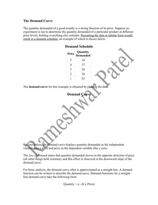
1. The Demand Curve
The quantity demanded of a good usually is a strong function of its price. Suppose an
experiment is run to determine the quantity demanded of a particular product at different
price levels, holding everything else constant. Presenting the data in tabular form would
result in a demand schedule, an example of which is shown below.
Demand Schedule
Quantity
Price
Demanded
5 10
4 17
3 26
2 38
1 53
The demand curve for this example is obtained by plotting the data:
Demand Curve
By convention, the demand curve displays quantity demanded as the independent
variable (the x axis) and price as the dependent variable (the y axis).
The law of demand states that quantity demanded moves in the opposite direction of price
(all other things held constant), and this effect is observed in the downward slope of the
demand curve.
For basic analysis, the demand curve often is approximated as a straight line. A demand
function can be written to describe the demand curve. Demand functions for a straight-
line demand curve take the following form:
Quantity = a - (b x Price)

2. where a and b are constants that must be determined for each particular demand curve.
When price changes, the result is a change in quantity demanded as one moves along the
demand curve.
Shifts in the Demand Curve
When there is a change in an influencing factor other than price, there may be a shift in
the demand curve to the left or to the right, as the quantity demanded increases or
decreases at a given price. For example, if there is a positive news report about the
product, the quantity demanded at each price may increase, as demonstrated by the
demand curve shifting to the right:
Demand Curve Shift
A number of factors may influence the demand for a product, and changes in one or more
of those factors may cause a shift in the demand curve. Some of these demand-shifting
factors are:
• Customer preference
• Prices of related goods
o Complements - an increase in the price of a complement reduces demand,
shifting the demand curve to the left.
o Substitutes - an increase in the price of a substitute product increases
demand, shifting the demand curve to the right.
• Income - an increase in income shifts the demand curve of normal goods to the
right.
• Number of potential buyers - an increase in population or market size shifts the
demand curve to the right.
• Expectations of a price change - a news report predicting higher prices in the
future can increase the current demand as customers increase the quantity they
purchase in anticipation of the price change.
The Supply Curve

3. Price usually is a major determinant in the quantity supplied. For a particular good with
all other factors held constant, a table can be constructed of price and quantity supplied
based on observed data. Such a table is called a supply schedule, as shown in the
following example:
Supply Schedule
Quantity
Price
Supplied
1 12
2 28
3 42
4 52
5 60
By graphing this data, one obtains the supply curve as shown below:
Supply Curve
As with the demand curve, the convention of the supply curve is to display quantity
supplied on the x-axis as the independent variable and price on the y-axis as the
dependent variable.
The law of supply states that the higher the price, the larger the quantity supplied, all
other things constant. The law of supply is demonstrated by the upward slope of the
supply curve.As with the demand curve, the supply curve often is approximated as a
straight line to simplify analysis. A straight-line supply function would have the
following structure:
Quantity = a + (b x Price)
where a and b are constant for each supply curve.

4. A change in price results in a change in quantity supplied and represents movement along
the supply curve.
Shifts in the Supply Curve
While changes in price result in movement along the supply curve, changes in other
relevant factors cause a shift in supply, that is, a shift of the supply curve to the left or
right. Such a shift results in a change in quantity supplied for a given price level. If the
change causes an increase in the quantity supplied at each price, the supply curve would
shift to the right:
Supply Curve Shift
There are several factors that may cause a shift in a good's supply curve. Some supply-
shifting factors include:
• Prices of other goods - the supply of one good may decrease if the price of
another good increases, causing producers to reallocate resources to produce
larger quantities of the more profitable good.
• Number of sellers - more sellers result in more supply, shifting the supply curve
to the right.
• Prices of relevant inputs - if the cost of resources used to produce a good
increases, sellers will be less inclined to supply the same quantity at a given price,
and the supply curve will shift to the left.
• Technology - technological advances that increase production efficiency shift the
supply curve to the right.
• Expectations - if sellers expect prices to increase, they may decrease the quantity
currently supplied at a given price in order to be able to supply more when the
price increases, resulting in a supply curve shift to the left.
Supply and Demand
The market price of a good is determined by both the supply and demand for it. In 1890,
English economist Alfred Marshall published his work, Principles of Economics, which

5. was one of the earlier writings on how both supply and demand interacted to determine
price. Today, the supply-demand model is one of the fundamental concepts of economics.
The price level of a good essentially is determined by the point at which quantity
supplied equals quantity demanded. To illustrate, consider the following case in which
the supply and demand curves are plotted on the same graph.
Supply and Demand
On this graph, there is only one price level at which quantity demanded is in balance with
the quantity supplied, and that price is the point at which the supply and demand curves
cross.
The law of supply and demand predicts that the price level will move toward the point
that equalizes quantities supplied and demanded. To understand why this must be the
equilibrium point, consider the situation in which the price is higher than the price at
which the curves cross. In such a case, the quantity supplied would be greater than the
quantity demanded and there would be a surplus of the good on the market. Specifically,
from the graph we see that if the unit price is $3 (assuming relative pricing in dollars), the
quantities supplied and demanded would be:
Quantity Supplied = 42 units
Quantity Demanded = 26 units
Therefore there would be a surplus of 42 - 26 = 16 units. The sellers then would lower
their price in order to sell the surplus.
Suppose the sellers lowered their prices below the equilibrium point. In this case, the
quantity demanded would increase beyond what was supplied, and there would be a
shortage. If the price is held at $2, the quantity supplied then would be:
Quantity Supplied = 28 units
Quantity Demanded = 38 units

6. Therefore, there would be a shortage of 38 - 28 = 10 units. The sellers then would
increase their prices to earn more money.
The equilibrium point must be the point at which quantity supplied and quantity
demanded are in balance, which is where the supply and demand curves cross. From the
graph above, one sees that this is at a price of approximately $2.40 and a quantity of 34
units.
To understand how the law of supply and demand functions when there is a shift in
demand, consider the case in which there is a shift in demand:
Shift in Demand
In this example, the positive shift in demand results in a new supply-demand equilibrium
point that in higher in both quantity and price. For each possible shift in the supply or
demand curve, a similar graph can be constructed showing the effect on equilibrium price
and quantity. The following table summarizes the results that would occur from shifts in
supply, demand, and combinations of the two.
Result of Shifts in Supply and Demand
Equilibrium Equilibrium
Demand Supply
Price Quantity
+ + +
- - -
+ - +
- + -
+ + ? +
- - ? -
+ - + ?
- + - ?

7. In the above table, "+" represents an increase, "-" represents a decrease, a blank
represents no change, and a question mark indicates that the net change cannot be
determined without knowing the magnitude of the shift in supply and demand. If these
results are not immediately obvious, drawing a graph for each will facilitate the analysis.
Price Elasticity of Demand
An important aspect of a product's demand curve is how much the quantity demanded
changes when the price changes. The economic measure of this response is the price
elasticity of demand.
Price elasticity of demand is calculated by dividing the proportionate change in quantity
demanded by the proportionate change in price. Proportionate (or percentage) changes
are used so that the elasticity is a unit-less value and does not depend on the types of
measures used (e.g. kilograms, pounds, etc).
As an example, if a 2% increase in price resulted in a 1% decrease in quantity demanded,
the price elasticity of demand would be equal to approximately 0.5. It is not exactly 0.5
because of the specific definition for elasticity uses the average of the initial and final
values when calculating percentage change. When the elasticity is calculated over a
certain arc or section of the demand curve, it is referred to as the arc elasticity and is
defined as the magnitude (absolute value) of the following:
Q2 - Q1
( Q1 + Q2 ) / 2
P2 - P1
( P1 + P2 ) / 2
where
Q1 = Initial quantity
Q2 = Final quantity
P1 = Initial price
P2 = Final price
The average values for quantity and price are used so that the elasticity will be the same
whether calculated going from lower price to higher price or from higher price to lower
price. For example, going from $8 to $10 is a 25% increase in price, but going from $10
to $8 is only a 20% decrease in price. This asymmetry is eliminated by using the average
price as the basis for the percentage change in both cases.

8. For slightly easier calculations, the formula for arc elasticity can be rewritten as:
( Q2 - Q1 ) ( P2 + P1 )
( Q2 + Q1 ) ( P2 - P1 )
To better understand the price elasticity of demand, it is worthwhile to consider different
ranges of values.
Elasticity > 1
In this case, the change in quantity demanded is proportionately larger than the change in
price. This means that an increase in price would result in a decrease in revenue, and a
decrease in price would result in an increase in revenue. In the extreme case of near
infinite elasticity, the demand curve would be nearly horizontal, meaning than the
quantity demanded is extremely sensitive to changes in price. The case of infinite
elasticity is described as being perfectly elastic and is illustrated below:
Perfectly Elastic Demand Curve
From this demand curve it is easy to visualize how an extremely small change in price
would result in an infinitely large shift in quantity demanded.
Elasticity < 1
In this case, the change in quantity demanded is proportionately smaller than the change
in price. An increase in price would result in an increase in revenue, and a decrease in
price would result in a decrease in revenue. In the extreme case of elasticity near 0, the
demand curve would be nearly vertical, and the quantity demanded would be almost
independent of price. The case of zero elasticity is described as being perfectly inelastic.

9. Perfectly Inelastic Demand Curve
From this demand curve, it is easy to visualize how even a very large change in price
would have no impact on quantity demanded.
Elasticity = 1
This case is referred to as unitary elasticity. The change in quantity demanded is in the
same proportion as the change in price. A change in price in either direction therefore
would result in no change in revenue.
Applications of Price Elasticity of Demand
The price elasticity of demand can be applied to a variety of problems in which one wants
to know the expected change in quantity demanded or revenue given a contemplated
change in price.
For example, a state automobile registration authority considers a price hike in
personalized "vanity" license plates. The current annual price is $35 per year, and the
registration office is considering increasing the price to $40 per year in an effort to
increase revenue. Suppose that the registration office knows that the price elasticity of
demand from $35 to $40 is 1.3.
Because the elasticity is greater than one over the price range of interest, we know that an
increase in price actually would decrease the revenue collected by the automobile
registration authority, so the price hike would be unwise.

10. Factors Influencing the Price Elasticity of Demand
The price elasticity of demand for a particular demand curve is influenced by the
following factors:
• Availability of substitutes: the greater the number of substitute products, the
greater the elasticity.
• Degree of necessity or luxury: luxury products tend to have greater elasticity than
necessities. Some products that initially have a low degree of necessity are habit
forming and can become "necessities" to some consumers.
• Proportion of income required by the item: products requiring a larger portion of
the consumer's income tend to have greater elasticity.
• Time period considered: elasticity tends to be greater over the long run because
consumers have more time to adjust their behavoir to price changes.
• Permanent or temporary price change: a one-day sale will result in a different
response than a permanent price decrease of the same magnitude.
• Price points: decreasing the price from $2.00 to $1.99 may result in greater
increase in quantity demanded than decreasing it from $1.99 to $1.98.
Point Elasticity
It sometimes is useful to calculate the price elasticity of demand at a specific point on the
demand curve instead of over a range of it. This measure of elasticity is called the point
elasticity. Because point elasticity is for an infinitesimally small change in price and
quantity, it is defined using differentials, as follows:
dQ
Q
dP
P
and can be written as:
dQ P
dP Q
The point elasticity can be approximated by calculating the arc elasticity for a very short
arc, for example, a 0.01% change in price.
In the previous section, supply and demand curves were drawn as straight lines. This is a
simplification, as we are assuming that the rate of change of demand or supply is the
same for all prices in the market.

11. Many goods have demand curves that look like this.
At some prices, a small change in price may cause a
large change in the quantity demanded.
This shown in the diagram as the movement from
Pe to Pe1; a small change in price which causes an
even larger percentage decrease in quantity
demanded (from Qe to Qe1.
The price elasticity of demand refers to the relationship between changes in price and
the subsequent change in quantity demanded. Economists are very interested in elasticity.
Calculating it will answer important questions like : if price rises by a certain amount,
by how much will demand fall, and total revenue change?
We use the Greek letter ''eta'' or η
To make the model easier to understand, we will continue using straight lines for the
demand and supply curves. What we will now look at is the slope of these curves: are the
curves ''flat'' or ''steep''? Be aware, though, that there is no necessary reason for a demand
or supply curve to be a straight line.
There are three methods that can be used to measure elasticity. The simplest is called the
total outlays method
Elasticity - The Total Outlays Method - 4
A simple method of measuring the price elasticity of demand is the total outlays
method. This method is only an approximate method of determining elasticity. The most

12. accurate method is the arc method of elasticity, which will be outlined later in this
section.
The ''total outlays'' method has two steps.
The first is to prepare a total outlay or total revenue table for the good or service under
investigation. The second step is to look at the change in total revenue received and
compare it with the direction of the price change that caused the change in total revenue.
Inelastic Demand - 10
If a given change in price causes a smaller
Qo, the initial quantity demanded is proportionate Q1, the new quantity demanded, is the
20,000 litres; change in quantity demanded, then
Demand for The is inelastic : petrol has no close500 litres,service is said toreduce their
19,500 litres.petrolchange in quantity demanded the substitute.on an initial demand level of
demand for is good or Motorists can be inelastic.
usage of their=car, and decrease.
20,000 litres a 2.5% perhaps drive fewer kilometres, but they can not fill their ''tank''
with water! In the diagram to your left, Po, the initial price is 65
The price elasticity of demand for cents perdefined asP1, the new price, is 75 in quantity
petrol is litre, and the percentage change cents per
Motorists can convert the percentage change in price. (Ignore any (whichsigns). In this
demanded divided by their cars to run onaliquified per litre increase.
litre; 10 cent petroleum gas minus is considerably
cheaper than price elasticity conversion cost / high. Petrol does have a substitute; but
example, the petrol), but the of petrol is 2.5%is 15% = 0.167.
LPG is not a close substitute.
Goods with price elasticities less than 1.0 are called inelastic.
Governments like to tax goods with inelastic demand curves. The diagram illustrates the
effect of a 10 cents per litre tax; a shift of the Supply Curve from S to S1. Petrol station
The percentage change in pricein sales; but per litre / 65 cents per litre =small. increase.
owners will notice a small fall is 10 cents the effect on their profits is a 15%
Governments do not like to be accused of driving small business out of business!
Other goods with high levels of taxation include alcohol and cigarettes: both very
inelastic.
Calculate the percentage increase in price, and the percentage decrease in quantity sold.
Calculate the price elasticity of ''Moo''.

13. Perfectly Inelastic Demand - 15
To have a situation where the Demand curve is a
vertical line is to think of a good where a certain
quantity is demanded, regardless of the price.
Heroin would be the closest ''real life'' example of
such a good. Addicts will pay anything for their ''fix''.
Factors Effecting the Elasticity of Demand - 20
Good with close substitutes tend to have elastic demand curves. The demand for good
''A'' is ''price sensitive'' to changes in the price of good ''B'', because they both satisfy the
same want. The demand for one brand of butter will vary, if another brand is put on
''special'' at your local supermarket.
''Necessities'' tend to have inelastic demand curves. If households see a good as essential
to daily living, demand for the good will be ''price insensitive''. For example, if the price
of milk rose by 50 cents a litre, demand for milk would not change greatly. All
households want milk.
Luxuries on the other hand tend to have elastic demand curves. If soft drinks are put on
''special'' at your local supermarket, and their price is lowered, demand for them will rise
markedly. Part of this ''necessities'' versus ''luxuries'' distinction is based on the cost of
the item. Many necessities are inexpensive: they have low prices - a loaf of bread, a litre
of milk, a box of matches, all only cost a very small part of your available disposable
income. An increase in the price of a litre of milk of 50 cents is still ''small change'' for
many consumers, and they will continue to demand milk at the same levels as they did
before the price rise. Luxuries on the other hand can be very expensive and cost a large
part of your available disposable income. You may decide not to buy that French
champagne to celebrate a birthday, if the price rises from $30 to $32. The price of $30 is
already a large enough disincentive.
Some goods are habit forming, or addictive. Cigarettes are a clear example. Once
''hooked'', the average smoker will continue to pay more and more for cigarettes, as
governments increase taxes on tobacco. Very few smokers give up smoking because of
price increases; most give up for health reasons.

14. Advertising Elasticity of Demand
Advertising elasticity of demand is the measure of how advertising affects the demand of
a certain product. It is the percentage change in the sales of the advertised product as
opposed to the percentage change in its advertising expenses.
Cross elasticity of demand
From Wikipedia, the free encyclopedia
Jump to: navigation, search
In economics, the cross elasticity of demand and cross price elasticity of demand
measures the responsiveness of the quantity demanded of a good to a change in the price
of another good.
It is measured as the percentage change in quantity demanded for the first good that
occurs in response to a percentage change in price of the second good. For example, if, in
response to a 10% increase in the price of fuel, the quantity of new cars that are fuel
inefficient demanded decreased by 20%, the cross elasticity of demand would be
-20%/10% = -2.
The formula used to calculate the coefficient cross elasticity of demand is
or:
Two goods that complement each other show a negative cross elasticity of demand: as the
price of good Y rises, the demand for good X falls

15. In the example above, the two goods, fuel and cars(consists of fuel consumption), are
complements - that is, one is used with the other. In these cases the cross elasticity of
demand will be negative. In the case of perfect complements, the cross elasticity of
demand is infinitely negative.
Where the two goods are substitutes the cross elasticity of demand will be positive, so
that as the price of one goes up the quantity demanded of the other will increase. For
example, in response to an increase in the price of carbonated soft drinks, the demand for
non-carbonated soft drinks will rise. In the case of perfect substitutes, the cross elasticity
of demand is equal to infinity.
Where the two goods are complements the cross elasticity of demand will be negative, so
that as the price of one goes up the quantity demanded of the other will decrease. For
example, in response to an increase in the price of fuel, the demand for new cars will
decrease.
Where the two goods are independent, the cross elasticity demand will be zero: as the
price of one good changes, there will be no change in quantity demanded of the other
good.
When goods are substitutable, the diversion ratio - which quantifies how much of the
displaced demand for product j switches to product i - is measured by the ratio of the
cross-elasticity to the own-elasticity multiplied by the ratio of product i's demand to
product j's demand. In the discrete case, the diversion ratio is naturally interpreted as the
fraction of product j demand which treats product i as a second choice,[1] measuring how
much of the demand diverting from product j because of a price increase is diverted to
product i can be written as the product of the ratio of the cross-elasticity to the own-
elasticity and the ratio of the demand for product i to the demand for product j. In some
cases, it has a natural interpretation as the proportion of people buying product j who
would consider product i their `second choice.'
Yield elasticity of bond value
Yield elasticity of bond value is the percentage change in bond value divided by a one
per percentage change in the yield to maturity of the bond. This is equivalent to saying
the derivative of value with respect to yield times the (interest rate/value). This is equal to
the MacAulay Bond Duration times the discount rate, or the modified bond duration
times the interest rate.
If elasticity is below -1, or above 1 if the absolute number is used, it means that the
product of the two measures, Value times yield or the interest income for the period will
go down