Supervised Classifier LDA CH04 Practitioners Handbook Machine Learning

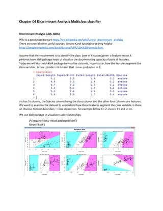
1. Chapter 04 Discriminant Analysis Multiclass classifier
Discriminant Analysis (LDA, QDA)
Wiki is a good place to start https://en.wikipedia.org/wiki/Linear_discriminant_analysis
There are several other useful sources. I found Kardi tutorial to be very helpful
https://people.revoledu.com/kardi/tutorial/LDA/LDA%20Formula.htm.
Assume that the requirement is to identify the class (one of K classes)given a feature vector X.
partimat from klaR package helps us visualize the discriminating capacity of pairs of features.
Today we will start with klaR package to visualize datasets, in particular, how the features segment the
class variable. Let us consider iris dataset that comes preloaded in R.
iris has 5 columns, the Species column being the class column and the other four columns are features.
We want to examine the dataset to understand how these features segment the class variable. Is there
an obvious decision boundary – class separation. For example below X < Z, class is C1 and so on.
We use klaR package to visualiize such relationships.
if (!require(klaR)) install.packages('klaR')
library('klaR')

2. we start with
partimat(Species~Sepal.Length+Sepal.Width+Petal.Length+Petal.Width,data=iris,method="lda")
But two classes are represented by the same letter V so let us change it to remove the ambiguity.
iris.lda<-iris # let us make a copy and change the species names
iris.lda$Species<-ifelse(iris$Species=='virginica','Wirginica',
ifelse(iris$Species=='versicolor','VERSI','SETOSA'))
# we expect to see S,V and W in the regions
table(iris.lda$Species)
iris.lda$Species<-as.factor(iris.lda$Species)
partimat(Species~Sepal.Length+Sepal.Width+Petal.Length+Petal.Width,data=iris.lda,method="ld
a")

3. Here I have used the partimat function from klaR package over iris dataset as shown above.
Let us use Fisher's Linear Discriminant Analysis to classify the iris dataset.
Now let us try to understand one feature at a time and its relationship with Class variable using ISLR 4th
chapter equations: I have attached scan of the important equations below. This book is freely available
on the internet.

4. mu_lda <- function(X, y){ # Equation 4.15, for mu
data_est <- as.data.frame(cbind(X,y))
data_est$X <- as.numeric(as.character(data_est$X))
mu <- aggregate(data = data_est, X ~ y, FUN = "mean")
colnames(mu) <- c("y", "X")
return(mu) # class wise mean
}
pi_lda <- function(y){ #
Equation 4.16
pi_est <- table(y) / length(y)
return(as.matrix(pi_est))
} # class proportion

5. var_lda <- function(X, y, mu){ # Equation 4.15, for sigma**2
n <- length(X)
K <- length(unique(y))
k <- unique(y)
var_est <- 0
for (i in 1:K){
var_est <- sum((X[y == k[i]] - mu$X[k[i] == mu$y])^2) + var_est
#X[[X[y=='setosa']-mu$X[setosa==mu$y
}
var_est <- (1 / (n - K)) * var_est
return(var_est)
}
discriminant_lda <- function(X, pi, mu, var){# Equation 4.17
K <- length(unique(y))
k <- unique(y)
disc <- matrix(nrow = length(X), ncol = K)
colnames(disc) <- k
for (i in 1:K){
disc[ ,i] <- X * (mu$X[i] / var) - ((mu$X[i]^2) / (2 * var)) + log(pi[i])
}
disc <- as.data.frame(disc)
disc$predict <- apply(disc, 1, FUN = "which.max")
return(disc)
}
# the Species is the target variable, 5th
column in iris
y <- as.character(iris[ ,5])
pi_est <- pi_lda(y)
LDA makes the assumption the variances are the same across the feature vectors.
Let us run through the feature vector, one by one, and estimate their ability to predict using the mean
and variance of a that feature.
X <- iris[ ,1] # we are reducing our feature space to be univariate

6. mu_est_1 <- mu_lda(X, y)
var_est_1 <- var_lda(X, y, mu_est_1)
discriminant_est_1 <- discriminant_lda(X, pi_est, mu_est_1, var_est_1)
table( iris$Species,discriminant_est_1$predict)
X <- iris[ ,2]
mu_est_2 <- mu_lda(X, y)
var_est_2 <- var_lda(X, y, mu_est_2)
discriminant_est_2 <- discriminant_lda(X, pi_est, mu_est_2, var_est_2)
table( iris$Species,discriminant_est_2$predict)
X <- iris[ ,3]
mu_est_3 <- mu_lda(X, y)
var_est_3 <- var_lda(X, y, mu_est_3)
discriminant_est_3 <- discriminant_lda(X, pi_est, mu_est_3, var_est_3)
table( iris$Species,discriminant_est_3$predict)
X <- iris[ ,4]
mu_est_4 <- mu_lda(X, y)
var_est_4 <- var_lda(X, y, mu_est_4)
discriminant_est_4 <- discriminant_lda(X, pi_est, mu_est_4, var_est_4)
table( iris$Species,discriminant_est_4$predict)

7. The best performance (or lowest error) we get is 6 misclassifications
# can there be a meta learner to combine these single feature classifier
predictions<-data.frame(actual=iris$Species,pred1=discriminant_est_1$predict,
pred2=discriminant_est_2$predict,pred3=discriminant_est_3$predict,
pred4=discriminant_est_4$predict)
predictions
We can see that a single attribute can detect species as well as it does, atleast for the iris dataset.
Let us now consider an implementation of ..equation ISLR 4.19 from implemented by Professor Dalal
(Columbia.edu).
# Let us setup three distinct data.frames
default_setosa<-iris[iris[,5]=='setosa',]
default_virginica<-iris[iris[,5]=='virginica',]
default_versicolor<-iris[iris[,5]=='versicolor',]
# for each class, let us compute the mean for each feature
mu_setosa<-apply(default_setosa[,1:4],2,mean)

8. mu_virginica<-apply(default_virginica[,1:4],2,mean)
mu_versicolor<-apply(default_versicolor[,1:4],2,mean)
# for each class, let us compute the cov
sigma_setosa<-cov(default_setosa[,1:4])
sigma_virginica<-cov(default_virginica[,1:4])
sigma_versicolor<-cov(default_versicolor[,1:4])
# for each class, get the number of rows
n_setosa<-dim(default_setosa)[1]
n_virginica<-dim(default_virginica)[1]
n_versicolor<-dim(default_versicolor)[1]
# let us compute the pooled covariance
sigma_all<-((n_setosa-1)*sigma_setosa+(n_virginica-1)*sigma_virginica+(n_versicolor-
1)*sigma_versicolor)/(n_setosa+n_virginica+n_versicolor-3) #pooled Cov matrix-
# a vector of means
mu<-cbind(mu_setosa,mu_virginica,mu_versicolor)
# prior probabilities for each class
pi.vec <- rep(0,3) # why not just pi?
pi.vec[1] <- sum((iris$Species=='setosa'))/nrow(iris)
pi.vec[2] <- sum((iris$Species=='virginica'))/nrow(iris)
pi.vec[3] <- sum((iris$Species=='versicolor'))/nrow(iris)
# the discriminant function implementing 4.19 from ISLR
my.lda<-function(pi.vec,mu,Sigma,x){
x.dims <- dim(x)
n <- x.dims[1]
Sigma.inv <- solve(Sigma) #Find inverse of Sigma
out.prod <- rep(1,n) #all items initiated to be negative
# equation 4.19 from ISLR Sixth Printing Page 157
discrim.setosa <- apply(x,1,function(y) y %*% Sigma.inv %*% mu[,1]
- 0.5*t(mu[,1]) %*% Sigma.inv %*% mu[,1] + log(pi.vec[1]))
discrim.virginica <- apply(x,1,function(y) y %*% Sigma.inv %*% mu[,2]
- 0.5*t(mu[,2]) %*% Sigma.inv %*% mu[,2] + log(pi.vec[2]))
discrim.versicolor <- apply(x,1,function(y) y %*% Sigma.inv %*% mu[,3]
- 0.5*t(mu[,3]) %*% Sigma.inv %*% mu[,3] + log(pi.vec[3]))
probs<-data.frame(p1=discrim.setosa,p2=discrim.virginica,p3=discrim.versicolor)
out.prod<-unlist(apply(probs,1,which.max))
return(out.prod)
}
pred_default_all<-my.lda(pi.vec,mu,sigma_all,iris[,1:4])

9. Performance (accuracy) has increased with our MV implmentation. We now have only 3
misclassifications. In contrast, with univariate model, the lowest misclassifications we achieved was 6.
Let us compute the other metrics, precision,recall,specificity,sensitivity, using caret package.
This concludes our exploration of parametric classifiers.
Concluding Remarks
These are supervised learners – first they learn using samples with labels , during the induction or
learning phase and then during the generalization phase (aka scoring) label a unlabeled observation
when presented. Logistic,NB and LDA all assume that data is distributed according to some known
distribution. A normal distribution is fully defined by the mean and the variance. Most other common
distributions are defined by a few parameters. Hence, these are called parametric methods. Logistic is
binary classifier (1 and 0) and seeks a linear seperation boundary. NaiveBayes and LDA are multiclass. –
LDA is linear classifier because 4.17 is linear in x. Here we explained using iris dataset. In the RMD we
will implement using heart dataset.
Logistic Regression transforms the features using logit (sigmoid function) and estimates the betas using
Gradient Descent or MLE or other optimization techniques.

10. NaiveBayes assumes features are class-conditionally independent and is easily derived from Bayes
theorem. All three parametric methods we have covered are Bayesian Estimators in that they assign the
class with the highest probability.
A wikipedia offers a crisp definition of these approaches
It will not be complete review of parametric classifiers without mentioning the two families of
parametric estimators – generative and discriminative, a brief review follows. We can reason about
Parametric classifiers whether they are computing joint probabilities or conditional probabilities.
Classifiers that compute p(x,y) are generative – as you can generate new observations given p(x,y). On
the other hand classifiers that compute p(x|y) are discriminative.
Another useful definition is based on what the classifier does. Does it determine a boundary that
separates one class from the other. If it does it is a discriminative classifier. Given a decision boundary
we cannot generate new observations. It is good to know the lingo and to appreciate p(x|y) is easier
than computing p(x,y). NaiveBayes is considered generative and Logistic Regression is considered
discriminative.
We will now go onto evaluate non-parametric methods namely kNN – k Nearest Neighbor and Decision
Tree and support vector machines . Practice alone makes perfect.