SlideShare una empresa de Scribd logo
1 de 7
Descargar para leer sin conexión
Letters
https://doi.org/10.1038/s41550-017-0262-6
© 2017 Macmillan Publishers Limited, part of Springer Nature. All rights reserved.
1
​Mullard Space Science Laboratory, Department of Space and Climate Physics, University College London, Holmbury St Mary, Dorking, Surrey RH5 6NT, UK.
2
​The Centre for Planetary Science at UCL/Birkbeck, Gower Street, London WC1E 6BT, UK. 3
​Harvard-Smithsonian Center for Astrophysics, Smithsonian
Astrophysical Observatory, Cambridge, 02138 MA, USA. 4
​Department of Physics, Lancaster University, Lancaster, LA1 4YW UK. 5
​Department of Physics
and Astronomy, University of Southampton, Southampton, SO17 1BJ UK. 6
​NASA Marshall Space Flight Center, Huntsville, 35811 AL, USA. 7
​Laboratoire de
Physique Atmosphérique et Planétaire, Université de Liège, Liège, B-4000, Belgium. 8
​Center for Space Physics, Boston University, Boston, 02215 MA, USA.
9
​Space Science and Engineering Division, Southwest Research Institute, San Antonio, 78238 Texas, USA. 10
​Jet Propulsion Laboratory, California Institute of
Technology, Pasadena, CA 91109, USA. 11
​Kavli Institute for Astrophysics and Space Research, Massachusetts Institute of Technology, Cambridge, 02109
MA, USA. 12
​Escuela Técnica Superior de Ingeniería — ICAI, Universidad Pontificia Comillas, Madrid, 28015 Spain. *e-mail: w.dunn@ucl.ac.uk
Auroral hot spots are observed across the Universe at dif-
ferent scales1
and mark the coupling between a surrounding
plasma environment and an atmosphere. Within our own
Solar System, Jupiter possesses the only resolvable example
of this large-scale energy transfer. Jupiter’s northern X-ray
aurora is concentrated into a hot spot, which is located at the
most poleward regions of the planet’s aurora and pulses either
periodically2,3
or irregularly4,5
. X-ray emission line spectra
demonstrate that Jupiter’s northern hot spot is produced by
high charge-state oxygen, sulfur and/or carbon ions with an
energy of tens of MeV (refs 4–6
) that are undergoing charge
exchange. Observations instead failed to reveal a similar
feature in the south2,3,7,8
. Here, we report the existence of a
persistent southern X-ray hot spot. Surprisingly, this large-
scale southern auroral structure behaves independently of its
northern counterpart. Using XMM-Newton and Chandra X-ray
campaigns, performed in May–June 2016 and March 2007, we
show that Jupiter’s northern and southern spots each exhibit
different characteristics, such as different periodic pulsations
and uncorrelated changes in brightness. These observations
imply that highly energetic, non-conjugate magnetospheric
processes sometimes drive the polar regions of Jupiter’s day-
side magnetosphere. This is in contrast to current models of
X-ray generation for Jupiter9,10
. Understanding the behaviour
and drivers of Jupiter’s pair of hot spots is critical to the use
of X-rays as diagnostics of the wide range of rapidly rotating
celestial bodies that exhibit these auroral phenomena.
The XMM-Newton and Chandra X-ray observatories conducted
~12 hour (1.2 Jupiter rotations) observations of Jupiter on 24 May
(both XMM and Chandra) and 1 June (Chandra only) 2016 and a
5 hour observation (0.5 Jupiter rotations) on 3 March 2007 (both
Chandra and XMM—see  Supplementary Material for analysis).
At these times, Jupiter’s tilt provided excellent visibility of both
Jupiter’s northern and southern polar auroras. The combination of
Chandra’s High Resolution Camera (HRC-2016 observations) and
Advanced CCD Imaging Spectrometer (ACIS-2007 observation)
and XMM-Newton’s Reflection Grating Spectrometer (RGS) and
European Photon Imaging Camera (EPIC) together provided high
spatial and spectral resolution X-ray observations in the energy
band 0.2–2.0 keV. The entire observable disk of Jupiter fits within
both the Chandra-HRC and XMM-Newton-EPIC field of view, so
that in 2016 both instruments provided continuous coverage of the
planet for more than one Jupiter rotation and could observe both
northern and southern auroral regions, as they rotated into view.
Both Chandra and XMM-Newton time-tag each X-ray photon,
which, for Chandra HRC’s high spatial resolution, allows Jupiter’s
X-ray emissions to be connected with the latitude and longi-
tudes from which they originate. Unlike that of the Earth, where
observable surface features provide unique latitude–longitude
coordinate identifiers, Jupiter’s solid surface is not observable
and its layers of cloud rotate around the planet at different rates.
To apply a consistent coordinate reference frame to these obser-
vations, we therefore used the left-handed S3 coordinate system,
which rotates with Jupiter’s 9.925 h rotation. Projections of the
locations of these X-ray emissions on Jupiter’s poles reveal that
both Jupiter’s northern and southern X-ray auroral emissions are
concentrated into hot spots that persistently occur in the same S3
latitude–longitude locations (Fig. 1). These X-ray hot spots both
occur poleward of Jupiter’s main ultraviolet auroral oval, which is
known to be generated by magnetospheric process(es) between 15
and 50 Jupiter radii (RJ)11
. The southern spot (poleward of −​67°
latitude and between 30°–75° S3 longitude) occurs closer to its
respective geographic pole than the northern spot (60°–75° lati-
tude and 155°–180° S3 longitude2,5
). This explains how, in previ-
ously published X-ray observations2,3
, unfavourable viewing meant
the southern hot spot was obscured.
Figure 2 shows overlaid lightcurves from the northern and south-
ern hot spots to reveal the characteristic pulsations of each spot. At
times when both spots are on Jupiter’s observable disk (approximate
central meridian longitude (CML) 90°–120°), these lightcurves
show that the X-ray spots sometimes pulse together (for example
minute 460, 24 May), but that more than 50% of their pulses are
independent (for example minutes 420–450 and 470–500, 24 May).
This means that knowledge of whether one hot spot brightens does
not help to predict whether its counterpart also brightens.
The northern X-ray spot has been observed to pulse either irreg-
ularly4,5
or with regular periods of 12, 26 or 40–45 minutes (refs 2,3
).
To provide quantitative estimates of the periodicities in each of the
The independent pulsations of Jupiter’s northern
and southern X-ray auroras
W. R. Dunn   1–3
*, G. Branduardi-Raymont1
, L. C. Ray4
, C. M. Jackman   5
, R. P. Kraft3
, R. F. Elsner6
,
I. J. Rae   1
, Z. Yao   1,7
, M. F. Vogt   8
, G. H. Jones   1,2
, G. R. Gladstone9
, G. S. Orton10
, J. A. Sinclair   10
,
P. G. Ford11
, G. A. Graham   1
, R. Caro-Carretero   1,12
and A. J. Coates   1,2
Nature Astronomy | VOL 1 | NOVEMBER 2017 | 758–764 | www.nature.com/natureastronomy758
© 2017 Macmillan Publishers Limited, part of Springer Nature. All rights reserved.
LettersNATUre ASTrOnOMY
hot spots for these observations, a Fourier transform was performed
on the raw unsmoothed time series to produce power spectral den-
sity (PSD) plots (Fig. 3). These PSDs show that on both 24 May
and 1 June 2016 the southern spot pulsed with statistically signifi-
cant regular periods of 9–11 min. Both Chandra and XMM-Newton
independently observed this regular 9–11 min period on 24 May. A
northern 12 min periodicity in the X-ray brightness was previously
observed during a magnetospheric compression3
. The recurrence
of a 9–12 min and 40–45 min period2,3
across multiple observations
may suggest bimodal regular periodicity.
Surprisingly, whereas the 9–11 min southern spot period is
highly statistically significant in both observations (probability of
chance occurrence (PCO) 10−5
–10−7
), the northern spot pulsations
show no significant 11 min period on 24 May and only a low-signif-
icance 12-min period (PCO 10−2
) on 1 June. The north does exhibit
some lower-significance (PCO <​ 10−4
) 5–8 min periods, but these
are not consistent across hemispheres or instruments.
The periodicity is not the only characteristic that seems to behave
independently for each spot during these observations. The light-
curves (Fig. 2) show that the brightnesses of the two spots are also
uncorrelated. We observed 78 ±​ 9 X-ray photons from the southern
spot during the first Chandra X-ray Observatory (CXO) observa-
tion and 111 ±​ 11 X-ray photons during the second observation — a
~40% increase in X-ray emission. In contrast, we observed 298 ±​ 17
X-rays from the northern spot during the first observation, but only
189 ±​ 14 X-rays during the second; that is, the emission decreased
by ~40%.
Analysis of the XMM-Newton EPIC spectra (Supplementary
Information) shows that the dominant emissions from the north-
ern and southern aurora are from precipitating ions of O7+,8+
and
S6+,…,14+
and/or C5+,6+
and therefore relate to downward current
regions9,10
. To identify more precisely the sources for these precip-
itating ions and the associated downward currents, we use a flux
equivalence mapping model12,13
to connect magnetic field lines in
the ionosphere with the equatorial magnetosphere (using the north-
ern Grodent anomaly12
and southern VIP414
models). Our northern
distribution (Fig. 4) matches the one observed previously3,8
, with
the precipitating ions originating beyond 60RJ and between 10:00
and 19:00 magnetospheric local time (MLT). The southern spot
also maps beyond 60RJ, but is concentrated between 10:00 and 14:00
MLT, and it then rotates out of view before we have the opportu-
nity to observe it mapping to later MLTs. If, as with the northern
spot, southern X-rays continued to be triggered when the spot maps
along the afternoon–dusk flank, this emission would be unobserv-
able from the Earth, addressing why fewer X-rays are almost always
observed from the south15
. This broader local time origin for the
northern spot may also explain the distinctive temporal signatures
shown in Figs. 2 and 3, as different plasma populations, physical
180°
270°
X-raysper2°
X-raysper2°
90°
14
12
12
10
10
8
8
6
6
270°90°
270°90°
12
10
8
6
4
2
0
4
3
2
1
0
0.525
0.500
0.475
0.450
0.425
0.400
0.375
0.625
0.600
0.575
0.550
0.525
0.500
0.475
270°90°
North
North South
South
180°
0°
0°
0°
0°
180°
180°
Fig. 1 | Polar projections of Jupiter’s northern and southern X-ray auroras. Top row: Projections centred on Jupiter’s north (left) and south (right) poles.
The projections combine 11–12 h X-ray observations of Jupiter on 24 May and 1 June 2016. Colours indicate the number of X-rays observed with the
Chandra HRC in bins of 1.5° by 1.5° of S3 latitude–longitude. Dotted lines of longitude radiate from the pole, increasing clockwise (anti-clockwise) for
the north (south) pole in increments of 30° from 0° at the bottom (top). Concentric dotted circles outward from the pole represent 10º increments in
latitude. Thin gold contours with white text labels indicate the VIP414
model magnetic field strength in Gauss. Thick gold contours show the magnetic field
ionospheric footprints of field lines intersecting the Jovigraphic equator at 5.9RJ (Io’s orbit), 15RJ and 50RJ (refs 12,13
) from equator to pole, respectively.
The location of Jupiter’s dipole magnetic pole is given by the red dot. These projections reveal that the X-ray aurora is clustered into a hot spot at both
poles. The northern spot is between 155° and 180° longitude and 60° and 75° latitude, as previously observed2,3,5,7,8
. The southern spot is longitudinally
broader (30°–75°) and poleward of 67° latitude, located closer to the geographic pole. Projection effects lead regions of 1.5° latitude by 1.5° longitude near
the poles to appear longer in latitude than in longitude, which leads to the streak-like morphology. This is an artefact of the projection and not a physical
feature. Bottom row: North (left) and south (right) polar projection exposure maps. The colour bar indicates the fraction of the total observing time during
which each region was observed. These show that the clustering of X-rays in the hot spots is not due to additional observation time in these regions.
Nature Astronomy | VOL 1 | NOVEMBER 2017 | 758–764 | www.nature.com/natureastronomy 759
© 2017 Macmillan Publishers Limited, part of Springer Nature. All rights reserved.
Letters NATUre ASTrOnOMY
processes and/or acceleration may be involved along the dusk flank
relative to the noon magnetopause.
Jupiter’s magnetopause has a typical subsolar standoff distance
of 60–90RJ, depending on the dynamic pressure of the solar wind16
.
The flux equivalence mapping12,13
is calculated using magnetic field
observations averaged over all solar wind conditions so that emis-
sion mapping beyond 60RJ could indicate ions precipitating on
closed field lines from the outer magnetosphere and/or field lines
that are open to the solar wind, depending on solar wind conditions
at the time. Of the X-rays in each spot, 30–60% of photons mapped
to locations beyond the modelled expanded magnetopause location
and are thus not shown on Fig. 4.
Currently, the favoured explanation for the northern X-ray hot
spot is that it is the signature of Jupiter’s northern cusp3,5,7,8
: that is, the
dayside region of the magnetosphere that is open to the solar wind.
It might therefore follow that Jupiter’s southern spot locates Jupiter’s
southern cusp. For fast solar wind, X-rays are proposed to be gener-
ated in this cusp region by vortical flows from pulsed reconnection at
the dayside magnetopause9
. These flows change the downward cur-
rents into the ionosphere and produce field-aligned potential drops
of the order of megavolts9,10
. These potential drops can accelerate
~2 keV O2+
ions17
in the outer magnetosphere to the 16–32 MeV
(1–2 MeV per atomic mass unit, amu) needed for Jupiter’s atmo-
sphere to strip electrons and produce the observed O6+
X-ray K-shell
line emissions4,6,9
. If reconnection pulses occur at Jupiter’s Alfvén-
wave transit timescale of about 30–50 min, it is suggested that this
mechanism could also explain the 45 min X-ray periodicity9
.
However, a varied set of challenges needs to be overcome in order
for pulsed dayside reconnection to explain the generation of Jupiter’s
X-ray hot spots in the observation reported here: (1) the 9–12 min
periodicity observed is on a shorter timescale than predicted; (2) for
subsolar point reconnection, both poles should pulse periodically
in-phase9
, but the dominant periodicity in the south does not also
dominate the northern lightcurves (Fig. 3) and north–south pulsa-
tions often appear to be independent of one another (Fig. 2); (3) the
overall brightness of the northern spot seems to be uncorrelated to
the overall brightness of the southern spot; and (4) a more general
challenge to the proposed pulsed reconnection mechanism is that
it explains X-ray emissions during fast solar wind conditions, but
previously X-rays have also been observed during slow solar wind
conditions3,8
. To address these challenges, here we propose adapta-
tions and alternative mechanisms to explain the observed soft X-ray
hot spot emissions during these observations.
Differing pulsation periods for each pole could be produced
by orientations of the interplanetary magnetic field that do not
favour subsolar reconnection9
. At Saturn, tension associated with
east–west motion of field lines during off-equatorial reconnection
can produce transient non-conjugate enhancements in ultraviolet
polar auroral brightness by disrupting field-aligned currents in the
respective poles18
.
High-latitude antiparallel reconnection may also provide non-
conjugacy. Lobe reconnection has been debated19,20
as Jupiter’s
24 May 2016 CML (°)
40
North
South
North
South
60
50
40
30
Countsperks
20
10
0
350 400 450 500
Time (min)
550 650600
70 100 130 160 190 220
1 June 2016 CML (°)
40
60
50
40
30
Countsperks
20
10
0
50 100 150 200 250 300 350
Time (min)
70 100 130 160 190 220
Fig. 2 | X-ray aurora lightcurves. Chandra X-ray lightcurves from times
when the northern (blue) and southern (gold) hot spots were both
observable on 24 May 2016 (top) and 1 June 2016 (bottom). The visibility
as a fraction of maximum visibility for the northern (blue) and southern
(gold) hot spots is indicated by the dashed curves. CML is indicated across
the top, and minutes from the observation start times (10:23 and 11:32 ut,
respectively) are indicated on the bottom axis. The lightcurves are one-
minute binned, with six-minute moving-average smoothing.
24 May CXO southern hot spot
5
Period (min)
0
5
10
15
20
PSD
25
30
35
10–7
10–6
10–5
10–4
10–3
10–2
10–1
10 50 100
24 May CXO northern hot spot
5
Period (min)
0
5
10
15
20
PSD
25
30
35
10–7
10–6
10–5
10–4
10–3
10–2
10–1
10 50 100
1 June CXO southern hot spot
5
Period (min)
0
5
10
15
20
PSD
25
30
35
10–7
10–6
10–5
10–4
10–3
10–2
10–1
10 50 100
1 June CXO northern hot spot
5
Period (min)
0
5
10
15
20
PSD
25
30
35
10–7
10–6
10–5
10–4
10–3
10–2
10–1
10 50 100
24 May XMM southern hot spot
5
Period (min)
0
5
10
15
20
PSD
25
30
35
10–7
10–6
10–5
10–4
10–3
10–2
10–1
10 50 100
24 May XMM northern hot spot
5
Period (min)
0
5
10
15
20
PSD
25
30
35
10–7
10–6
10–5
10–4
10–3
10–2
10–1
10 50 100
Fig. 3 | X-ray aurora periodograms. PSD plots from fast Fourier transforms
of X-ray lightcurves from the southern (left) and northern (right) X-ray
hot spots in 2016. PSDs are shown from Chandra observations on
24 May (top), simultaneous XMM-Newton observations on 24 May
(middle) and from Chandra observations on 1 June (bottom). The dotted
horizontal lines show single-frequency PCO for the detected periods43
. The
lowest statistical significance and highest PCO of 10−1
is at the bottom of the
plot. The dashed red lines show the value obtained if photons from a steady
source were randomly distributed over the visibility period. Lightcurves
were extracted from 20–70° longitude and poleward of −​60° latitude for
the south and from 155–180° longitude and poleward of 60° latitude for the
northern hot spot. For XMM, with poorer spatial resolution and therefore
subject to increased contamination from the disk emission, the lightcurves
are extracted from the same time window as the Chandra observations.
Nature Astronomy | VOL 1 | NOVEMBER 2017 | 758–764 | www.nature.com/natureastronomy760
© 2017 Macmillan Publishers Limited, part of Springer Nature. All rights reserved.
LettersNATUre ASTrOnOMY
dominant solar-wind reconnection process. This is predominantly
because the planet’s immense size, rapid rotation and internal
plasma source lead to long relative timescales for return flows from
an Earth-like Dungey cycle, and, under certain conditions, suppress
dayside reconnection21
. For high-latitude reconnection, recon-
nected/closing lobe field lines may travel equatorward across the
cusp and into the dayside magnetosphere22,23
. This could explain
the large spatial extent of the X-ray spots. Asymmetric high-latitude
reconnection can also produce a persistent reconnection site over
one pole and a moving reconnection site over the other pole. This
may explain the contrasting regular 9–11 min X-ray period in the
south and irregular pulsations in the north. Subsolar dayside recon-
nection can produce X-rays from high-charge-state magnetosheath
or solar wind ions (such as O7+
) on open field lines, but these emis-
sions are calculated to be orders of magnitude fainter than the total
X-ray brightness observed9,10
. However, certain topologies of high-
latitude reconnection may offer additional acceleration mecha-
nisms, closing and dipolaring of stretched and/or twisted open field
lines or lobe field lines in the outer magnetosphere could energize
ions through Fermi acceleration.
Kelvin Helmholtz instabilities (KHIs) are perhaps one of the
most important large-scale instabilities that occur in coronal, mag-
netospheric and astrophysical environments, transferring large
quantities of energy, momentum and plasma between separate
plasma regimes. They are also thought to occur at Jupiter’s mag-
netopause21,24
, and they offer an alternative mechanism capable of
explaining the periodic X-ray signatures3,8
. For the Earth’s magne-
tosphere, KHIs can trigger magnetopause fluctuations and excite
compressional ultralow-frequency (ULF) magnetic field oscilla-
tions and field line resonances, driving standing Alfvén waves in
the ionosphere25,26
. At Jupiter, ULF waves have been observed with
10–20 min periodicity27,28
, the lower bound of which matches our
9–12 min X-ray pulsations. The periodicity of ULF oscillations
depends on the magnitude of the magnetospheric cavity, veloc-
ity shear and thickness of the interaction boundary. At Jupiter, the
size of the magnetosphere varies bimodally between compressed
and expanded states (respective standoff distances16
63-92RJ). This
could explain the bimodal 9–12 min and 40–45 min X-ray aurora
periodicity. If the thickness of the magnetopause boundary, size
of the magnetosphere and velocity shear were similar on 24 May
and 1 June, then KHI-driven Alfvén waves could produce recurring
periodicity. Moreover, KHIs could generate different brightening
in each pole by driving oppositely directed field-aligned currents
in each hemisphere through Ampere’s law. Traditional KHI studies
focus solely on the shear in the flow as the generation mechanism.
However, magnetic field orientation, plasma characteristics and
thickness of the magnetopause boundary all have critical roles to
play in generating wave modes along the boundary. It is for these
reasons that, contrary to expectations from planetary rotation,
KHIs are often observed along the dusk flank of the magnetospheres
of both Earth29
and Saturn30
, as well as the dawn sector, where
the velocity shear is largest. Indeed, at larger velocity shears, KHI
may also be stabilized30
. The prevalence and locations of KHIs,
alongside the possibility of KHI-generated acceleration of the
order of the MeV amu-1
required for the observed X-ray signatures,
remain to be fully explored at Jupiter. However, wave–particle inter-
actions, KHI-driven reconnection and/or modulation of current
systems and their associated potential drops are all possible accel-
eration mechanisms.
The southern X-ray spot rotates out of view while the northern
spot rotates into view, so that they are observable simultaneously
only when they approach opposite limbs of Jupiter’s observable
disk. If the two spots are globally driven, then arguably the simplest
explanation for the north–south differences is that magnetospheric
conditions changed with time and damped the 11 min southern
period. Whether the differences are due to changes with time or
North spot X-ray
South spot X-ray
Noon
100
100
50
50
B
J
0
0
–50
–50
x (RJ)
y(RJ)
–100
–100
Dawn
Dusk
Fig. 4 | Ionosphere–magnetosphere mapping for the X-ray hot spots with
accompanying schematic for a KHI driver. Top: Mapping13
of X-ray photon
emission located in the ionosphere to the equatorial magnetosphere source
regions for the northern (blue) and southern (gold) hot spots. The solid
red lines indicate Jupiter’s magnetopause, for an expanded 92RJ, standoff
distance (outer contour) and compressed 63RJ standoff distance (inner
contour)16
. We also note that even for the statistical location of the expanded
magnetopause, because of the substantial spatial extent of the hot spots,
30–60% of X-rays mapped beyond the magnetopause, meaning that their
origins cannot be identified by the model mapping, and they are not plotted
here. Bottom: Illustration of a possible source mechanism for the observed
hot spot emissions. KHIs along the magnetopause could produce field line
resonances that generate regular periodicity in the emissions. Further, these
field line resonances could vary bimodally with the compressed or expanded
states of Jupiter’s magnetosphere. These KHIs may also generate
non-conjugate north–south auroral signatures, as twisting of the magnetic
field line (illustrated in red, B) can generate inter-hemispheric currents
(green, J). Schematics for drivers relating to field line tension from the
Y-component of the Interplanetary Magnetic Field (IMF) or high latitude
reconnection can be found in ref. 18
and ref. 23
respectively.
Nature Astronomy | VOL 1 | NOVEMBER 2017 | 758–764 | www.nature.com/natureastronomy 761
© 2017 Macmillan Publishers Limited, part of Springer Nature. All rights reserved.
Letters NATUre ASTrOnOMY
due to differing polar dynamics, both auroral spots are fixed in the
planet’s rotating coordinate system, so localized magnetic condi-
tions may also play some part in ensuring that ion acceleration to
energies of the order of MeV amu–1
is produced only in the hot spots
and not in any other auroral region.
These findings also highlight possible multi-wavelength con-
nections for Jupiter’s aurora. Ultraviolet polar auroral flares31
sometimes coincide with X-ray brightenings5
and, like the X-ray
pulsations, quasi-periodically enhance on roughly a 10 min tim-
escale32
. Bright infrared auroral hot spots are also co-located with
the X-ray hot spots, which may suggest that the pulses of precipita-
tion of high-energy ions, and their associated drivers, provide an
important heating mechanism for Jupiter’s stratosphere down to the
10 mbar pressure level33
.
The independent behaviour of Jupiter’s pair of soft X-ray hot
spots during these observations raises fundamental questions about
what processes at rapidly rotating magnetospheres produce these
auroras. For Jupiter, the spectral signatures of the precipitating ions
suggest that the spots locate Jupiter’s downward currents10
and may
identify the northern and southern cusps9
. However, the observed
distinctive behaviour could be indicative of non-equatorial recon-
nection, magnetopause-driven ULF waves, tail reconnection or
local magnetic conditions at each polar region. Over the coming
2 years, X-ray observing campaigns in conjunction with NASA’s
Juno mission will offer the opportunity to determine whether the
independent behaviour that we report here is commonplace or is
unique to the observations presented here. Critically, they will help
to identify the magnetospheric conditions and auroral processes
that are able to generate Jupiter’s highest-energy emissions and the
seemingly independent behaviour of the northern and southern
soft X-ray hot spots.
Method
Observation times. For all previously published X-ray campaigns with
Chandra2,3,5,7,8
and XMM-Newton (XMM)4,8,34,35
, the viewing geometry favoured
observations of the northern aurora. At these times, the sub-Earth latitudes of
0.2°–3.9° and north pole distance angles of 18°–23° obscured visibility of the
geographic south pole (Supplementary Material). However, during summer 2016
and March 2007, the tilt of Jupiter relative to the X-ray instruments in Earth
orbit allowed clear X-ray observations of Jupiter’s southern geographic pole
(north pole angle of −​17° and −​16° respectively and sub-Earth latitude of −​1.7°
and −​3.3° respectively). It is this viewing geometry, which is rare in the legacy
X-ray observations of Jupiter (see Supplementary Materials), that permitted clear
observations of the southern X-ray hot spot.
The 2016 Chandra observations and XMM observation continuously
observed a total CML range of 425° and 482° respectively during the 11.7 h
Chandra observations (1.17 Jupiter rotations) and 12.3 h XMM observation (1.23
Jupiter rotations). The Chandra observations on 24 May and 1 June started with
a CML of 185° and 350° respectively and finished with a CML of 250° and 55°
respectively. The XMM-Newton observation on 24 May started with a CML of 175°
and finished with a CML of 297°.The Chandra ACIS 5 h observation on
3 March 2007 covered a CML range of 290°–110°. The entirety of Jupiter’s disk fits
within the field of view of both Chandra HRC and ACIS instruments and XMM-
Newton’s EPIC-PN instrument, permitting simultaneous observations of Jupiter’s
northern and southern hot spots during the CML window when both spots are
at least partially on the observed disk. However, we note that the southern spot is
rotating out of view when the Northern spot rotates into view, so that both spots
can only be simultaneously observed in their entirety between CMLs ~90°–120°,
and at these times there are still viewing geometry limitations and possible effects
produced by the viewing angle of precipitation and/or the angle at which the
X-rays are emitted.
Given that each observation continuously covered 1.2 Jupiter rotations, this
meant that, for both observations, Jupiter’s northern and southern hot spots were
observed at least once, and the 24 May (1 June) observation partially observed
Jupiter’s northern (southern) hot spot a second time. To ensure that we did not
artificially enhance the X-ray counts by including multiple visits to the same
spot (two visits to the north on 24 May and two to the south on 1 June), in each
observation we extracted counts only from the longest duration window of these
two possible observing windows. A table of the counts recorded by Chandra from
every observing window can be found in the Supplementary Information.
Supplementary Fig. 1 shows a projection onto the south pole from the Chandra
ACIS observation on 3 March 2007. To analyse the ACIS data, we applied a
correction to the effective area3,5
to account for the increased energy thresholds
applied within ACIS to circumvent optical light leaks through the optical blocking
filters. This observation had a lower observer co-latitude (Supplementary Table 1),
offering better visibility of the geographic south pole than the 2016 campaign.
Although the observations from the 2007 campaign were dimmer than those from
2016 and used a different instrument (Chandra ACIS instead of Chandra HRC),
the polar projection shows that the X-rays are again concentrated into the southern
hot spot and that this occurs from 70° latitude to the pole and between 30°–60°
S3 longitude. Studies of eight X-ray observations of the northern spot have shown
that, from observation to observation, the hot spot expands and contracts centred
on a persistent location3,8
. This may suggest that although the southern spot is
centred on the same location in 2007 and 2016, it also expands and contracts from
this location. Alternatively, the apparent expansion in the 2016 observations may
be a projection effect produced by the slightly poorer visibility of the region during
the 2016 observations relative to the 2007 observations.
Supplementary Fig. 2 quantifies the concentrations of X-rays shown in Fig. 1
and Supplementary Fig. 1. In the 2016 and 2007 observations, the southern
hot spot occurred in the same longitude range, suggesting that it is a persistent
feature of the southern X-ray aurora. We contrast the count concentrations in
the auroral zones with emission from fluoresced and scattered solar photons in
Jupiter’s equatorial atmosphere. This demonstrates that the distributions are not
produced by transient variations in the solar X-ray flux. If this were the case, then
the disk distributions might be expected to match the auroral distributions, and
they do not. We also plot error bars on the count measurements, highlighting the
significance of the spots’ longitudinal concentrations relative to the more uniform
equatorial emission.
Spectral analysis. We analysed the XMM-Newton EPIC-PN spectral data from
24 May to identify the source populations of the observed emissions. To do this,
we applied the standard high-energy astrophysics software packages including
XMM-SAS and XSPEC. XMM-Newton has lower spatial resolution than Chandra.
To circumvent this, we used the information from Chandra (from the overlapping
interval) on the spatial locations of the spots with visibility information from
NASA JPL Horizons ephemerides data to select times that corresponded to CML
ranges when the hot spots were on Jupiter’s observable disk. For XMM, for the
north (south) we extracted hot spot spectra from times when the CML ranges
were 60°–270° (300°–170°). The time intervals outside these windows were
checked to ensure that the X-ray emission was evenly distributed across Jupiter’s
entire disk and no significant auroral concentrations were lost. Given the dynamic
nature of the hot spots, we only used the longest observation window and did not
combine the shorter partial observation windows with this. This disregarding of
times when the hot spot was unobservable is an alteration from previous
spectral studies34,36
; it allowed us to minimize contamination from scattered solar
photons and provided a more accurate calculation of X-ray emission rates from
the aurora only.
Using the standard XMM-SAS package, we then selected the appropriate
source regions for the northern and southern aurora from a planet-centred image
and extracted the relevant spectral products (spectral data from source region,
spectral data from background region, effective area/auxiliary response and
redistribution matrix files). To ensure that there were sufficient counts to reliably
fit models, we binned the data into 10-channel energy bins. Using the XSPEC
modelling package, we then tested model fits for a combination of different
Gaussian lines and bremsstrahlung continuum to a non-background-subtracted
spectrum (Jupiter’s disk blocks cosmic X-ray background emission5
).
To distinguish between auroral emission and potential contamination in
the polar region from fluorescence or scattering of solar photons in Jupiter’s
atmosphere, we also extracted the equatorial emission by using the same time
window as the auroral emissions. Given the low count rates, we used an equatorial
spectrum that covered the times when either hot spot was observable (sub-
observer longitude 300°–270°). Modelling of the equatorial spectrum showed
clearly distinctive features from the auroral emissions, indicating that the auroral
spectra were dominated by a different emission process (that is, not fluorescence
and scattering of solar photons).
A bremsstrahlung continuum was found not to give good fits for the northern
or southern auroral emissions, suggesting that both observed hot spots are
dominated by spectral lines from precipitating ions.
It was challenging to compare the northern and southern auroras directly
because of the low count levels for the south, but both the north (Supplementary
Table 6) and south (Supplementary Table 7) best-fit models feature a prominent
and well-defined O vii line centred on 568 eV and a high flux line in the region
where a range of sulfur and carbon lines are present. Both aurora best-fit models
also include a line at 430–470 eV where there are known C vi lines. Interestingly,
carbon is much more abundant in the solar wind than in Jupiter’s magnetosphere,
so this could suggest some direct solar wind precipitation. However, we note
that the 90% confidence errors on the fluxes for this specific line are 50% of the
measured flux for the north and more than this for the south. This 430–470 eV
line coincides with the lowest data point between 200 and 900 eV on the equatorial
spectrum, suggesting that it is not contamination from scattered solar photons, but
is a part of the auroral spectrum. The equatorial spectrum (Supplementary Fig. 5)
Nature Astronomy | VOL 1 | NOVEMBER 2017 | 758–764 | www.nature.com/natureastronomy762
© 2017 Macmillan Publishers Limited, part of Springer Nature. All rights reserved.
LettersNATUre ASTrOnOMY
does hint at the presence of a line at 400 eV, and we attempted to force model fits to
this, but these always led to worse fits and increased the reduced χ2
by at least 0.5.
As with previous Jovian disk analysis37
, we could attain a good fit (reduced χ2
of ~0.7) to the equatorial spectrum from 500–1,500 eV with a vmekal hot plasma
model using solar abundances with kT ≈​ 0.3 and flux of ~9 ×​ 10−7
photons cm−2
 s−1
.
To support comparison with the auroral emission (Supplementary Fig. 5), we
show a spectral model fitted with known solar spectrum lines38
: this shows that the
equatorial emission has a very different structure above 600 eV. If the observed and
modelled auroral emissions were due to solar contamination, then one would not
expect the auroral emissions to decrease above 600 eV, as they do.
Given that both the northern and southern auroras feature similar O vii, sulfur
and carbon lines, this may support a similar source population (as suggested by the
magnetospheric mapping to the noon magnetopause). This may also suggest that
any independent behaviour is locally driven.
The northern aurora is better fitted with the inclusion of an O viii line. More
energy is required to strip the additional electron in order to produce this line,
so the presence of the extra line may hint that a more energetic pulsation process
occurs in the observable northern aurora than in the south. This higher-charge-
state oxygen would, through charge exchange, subsequently lead to a cascade
of emissions from oxygen in lower charge states, which may explain further
differences between the oxygen spectra.
We note that the source regions for the two spectra are different (see Fig. 4),
which may explain some of the spectral differences (there may be changes in
acceleration, the driver process or the source ion population when moving from
the nose to the dusk flank), and the spectra do not cover the same time interval.
However, from this single north–south spectral comparison, it is difficult to
quantify the differences between the two spectra conclusively, as the intensities
of the southern spectral lines are a factor of 2–4 lower than for the north. Future
observations that provide good visibility of both poles will help to address and
interpret the spectral characteristics with more statistical certainty.
Lightcurves and XMM-Newton periodicity detection. For Chandra, the
1-min-binned lightcurves (Supplementary Fig. 2) from the northern spot were
produced by extracting X-rays from 155°–190° longitude and poleward of 60°
latitude. For the south, the 1-min-binned lightcurves (Supplementary Fig. 2)
were extracted from 20°–70° longitude and poleward of −​60° latitude. The
1-min-binned unsmoothed data were then fast Fourier transformed to produce
the PSDs shown in Fig. 4 of the main text. The lightcurves shown in Fig. 3 and
Supplementary Figs. 3 and 4 have been smoothed with a 6 minute moving average.
As with previous work2,3,5
, no moving-average smoothing was applied to generate
the Fourier transform frequency data. Supplementary Fig. 3 shows the complete
northern and southern auroral lightcurves for 24 May (Chandra and XMM-
Newton) and 1 June (Chandra) 2016.
The lightcurves from XMM-Newton’s EPIC contain more noise than the
Chandra HRC lightcurves because EPIC’s lower spatial resolution leads to
additional contamination from fluoresced and scattered solar X-ray photons on
Jupiter’s disk. This limited spatial resolution also prevents lightcurves from being
extracted based on S3 coordinate locations. As with the spectra, we therefore
extracted XMM-Newton auroral lightcurves from the auroral region, during the
same time window as the spectra — times when longitudes connected to the
X-ray hot spots were observable (CML 60°–270° or 300°–170° for the northern
and southern aurora respectively). The XMM-Newton southern (northern) PSDs
shown in Fig. 4 were therefore produced from Fourier transforms of the
300–500 min (450–700 min) unsmoothed data that generated these lightcurves.
The lightcurves for XMM-Newton are noisier, as the spatial resolution is not
as good as Chandra’s, and it was therefore not possible to select areas in S3
coordinates. Instead, we used auroral regions extracted from the disk of Jupiter,
which will include additional contamination from the disk emission. There are also
different energy-dependent responses and effective areas for XMM-Newton’s EPIC
and Chandra’s HRC and ACIS instruments, which may lead to differing lightcurve
morphology for each instrument.
Jupiter’s equatorial emissions are produced by solar photons that are fluoresced
and scattered in Jupiter’s atmosphere37,39,40
. Lightcurves and PSDs from the Jovian
equator on 24 May (day of year (DoY) 145) and 1 June (DoY 153) (Supplementary
Fig. 4) between −​30° and 30° latitude demonstrate that the periodic behaviour is
not present in the equatorial region and that there was not a significant variation in
the solar X-ray output (for example from solar flares) during the observations3,37,40
.
To statistically test how similar the PSDs were between each pole, each
instrument and each observation, we conducted a range of hypothesis tests and
calculated the P-value41
for each compared data set. Direct comparisons of a
hot spot PSD from the same pole but in different observations or instruments
produced relatively high P-values (Supplementary Table 4), suggesting that the
temporal behaviours of the emissions were similar. However, directly comparing
the northern PSDs with the southern PSDs produced low P-values, suggesting the
inter-hemisphere temporal behaviour is far less similar.
Supplementary Table 5 shows results from statistical analyses using the STA/
LTA algorithm42
to identify and characterize the three most prominent peaks in the
PSD plots in Fig. 4. This auto-detection of the peaks in the periodogram quantifies
and characterizes the strong 9–11 min period observed in the southern spot, which
is not also observed in the northern spot. We note, however, that a 5–8 min period
does seem to recur in the north.
Data availability. The data analysed within this paper are publicly available from
the Chandra and XMM-Newton Data Archives.
Received: 3 February 2017; Accepted: 25 August 2017;
Published online: 30 October 2017
References
	1.	 Hallinan, G. et al. Magnetospherically driven optical and radio aurorae at the
end of the stellar main sequence. Nature 523, 568–571 (2015).
	2.	 Gladstone, G. R. et al. A pulsating auroral X-ray hot spot on Jupiter. Nature
415, 1000–1003 (2002).
	3.	 Dunn, W. R. et al. The impact of an ICME on the Jovian X-ray aurora.
J. Geophys. Res. A Space Phys. 121, 2274–2307 (2016).
	4.	 Branduardi-Raymont, G. et al. A study of Jupiter’s aurorae with
XMM-Newton. Astron. Astrophys. 463, 761–774 (2007).
	5.	 Elsner, R. F. et al. Simultaneous Chandra X ray Hubble Space Telescope
ultraviolet, and Ulysses radio observations of Jupiter’s aurora. J. Geophys. Res.
Space Phys. 110, 1–16 (2005).
	6.	 Kharchenko, V., Bhardwaj, A., Dalgarno, A., Schultz, D. R. & Stancil, P. C.
Modeling spectra of the north and south Jovian X-ray auroras. J. Geophys.
Res. Space Phys. 113, 1–11 (2008).
	7.	 Branduardi-Raymont, G. et al. Spectral morphology of the X-ray emission
from Jupiter’s aurorae. J. Geophys. Res. Space Phys. 113, 1–11 (2008).
	8.	 Kimura, T. et al. Jupiter’s X-ray and EUV auroras monitored by Chandra,
XMM-Newton, and Hisaki satellite. J. Geophys. Res. Space Phys. 121,
2308–2320 (2016).
	9.	 Bunce, E. J., Cowley, S. W. H. & Yeoman, T. K. Jovian cusp processes:
Implications for the polar aurora. J. Geophys. Res. Space Phys. 109,
1–26 (2004).
	10.	Cravens, T. E. et al. Implications of Jovian X-ray emission for magnetosphere-
ionosphere coupling. J. Geophys. Res. Space Phys. 108, 1–12 (2003).
	11.	Cowley, S. W. H. & Bunce, E. J. Origin of the main auroral oval in Jupiter’s
coupled magnetosphere-ionosphere system. Planet. Space Sci. 49,
1067–1088 (2001).
	12.	Grodent, D. et al. Auroral evidence of a localized magnetic anomaly in
Jupiter’s northern hemisphere. J. Geophys. Res. Space Phys. 113, 1–10 (2008).
	13.	Vogt, M. F. et al. Improved mapping of Jupiter’s auroral features to
magnetospheric sources. J. Geophys. Res. Space Phys. 116, 1–24 (2011).
	14.	Connerney, J. E. P., Acuña, M. H., Ness, N. F. & Satoh, T. New models of
Jupiter’s magnetic field constrained by the Io flux tube footprint. J. Geophys.
Res. 103, 11929–11939 (1998).
	15.	Waite, J. H. et al. ROSAT observations of the Jupiter aurora. J. Geophys. Res.
99, 799–809 (1994).
	16.	Joy, S. P. et al. Probabilistic models of the Jovian magnetopause and bow
shock locations. J. Geophys. Res. Space Phys. 107, 1–17 (2002).
	17.	Bagenal, F. Empirical model of the Io plasma torus: Voyager measurements.
J. Geophys. Res. 99, 11043 (1994).
	18.	Meredith, C. J., Cowley, S. W. H., Hansen, K. C., Nichols, J. D. & Yeoman, T. K.
Simultaneous conjugate observations of small-scale structures in Saturn’s
dayside ultraviolet auroras: implications for physical origins. J. Geophys. Res.
Space Phys. 118, 2244–2266 (2013).
	19.	McComas, D. J. & Bagenal, F. Jupiter: a fundamentally different
magnetospheric interaction with the solar wind. Geophys. Res. Lett. 34,
1–5 (2007).
	20.	Cowley, S. W. H., Badman, S. V., Imber, S. M. & Milan, S. E. Comment on
‘Jupiter: a fundamentally different magnetospheric interaction with the solar
wind’ by D. J. McComas and F. Bagenal. Geophys. Res. Lett. 35, 1–3 (2008).
	21.	Desroche, M., Bagenal, F., Delamere, P. A. & Erkaev, N. Conditions at the
expanded Jovian magnetopause and implications for the solar wind
interaction. J. Geophys. Res. Space Phys. 117, 1–18 (2012).
	22.	Lockwood, M. & Moen, J. Reconfiguration and closure of lobe flux by
reconnection during northward IMF: possible evidence for signatures in
cusp/cleft auroral emissions. Ann. Geophys. 17, 996–1011 (1999).
	23.	Fuselier, S. A., Trattner, K. J., Petrinec, S. M. & Lavraud, B. Dayside magnetic
topology at the Earth’s magnetopause for northward IMF. J. Geophys. Res.
Space Phys. 117, 1–14 (2012).
	24.	Delamere, P. A. & Bagenal, F. Solar wind interaction with Jupiter’s
magnetosphere. J. Geophys. Res. Space Phys. 115, 1–20 (2010).
	25.	Mann, I. R. et al. Coordinated ground-based and Cluster observations of
large amplitude global magnetospheric oscillations during a fast solar wind
speed interval. Ann. Geophys. 20, 405–426 (2002).
	26.	Rae, I. J. et al. Evolution and characteristics of global Pc5 ULF waves
during a high solar wind speed interval. J. Geophys. Res. Space Phys. 110,
1–16 (2005).
	27.	Khurana, K. K. & Kivelson, M. G. Ultralow frequency MHD waves in
Jupiter’s middle magnetosphere. J. Geophys. Res. 94, 5241 (1989).
Nature Astronomy | VOL 1 | NOVEMBER 2017 | 758–764 | www.nature.com/natureastronomy 763
© 2017 Macmillan Publishers Limited, part of Springer Nature. All rights reserved.
Letters NATUre ASTrOnOMY
	28.	Wilson, R. J. & Dougherty, M. K. Evidence provided by galileo of ultra low
frequency waves within Jupiter’s middle magnetosphere. Geophys. Res. Lett.
27, 835–838 (2000).
	29.	Hasegawa, H. et al. Transport of solar wind into Earth’s magnetosphere
through rolled-up Kelvin–Helmholtz vortices. Nature 430, 755–758 (2004).
	30.	Ma, X., Stauffer, B., Delamere, P. A. & Otto, A. Asymmetric Kelvin–
Helmholtz propagation at Saturn’s dayside magnetopause. J. Geophys. Res.
Space Phys. 120, 1867–1875 (2015).
	31.	Bonfond, B. et al. Quasi-periodic polar flares at Jupiter: a signature of pulsed
dayside reconnections? Geophys. Res. Lett. 38, 1–5 (2011).
	32.	Nichols, J. D. et al. Response of Jupiter’s auroras to conditions in the
interplanetary medium as measured by the Hubble Space Telescope and Juno.
Geophys. Res. Lett. 44, 7643–7652 (2017).
	33.	Sinclair, J. A. et al. Independent evolution of stratospheric temperatures in
Jupiter’s northern and southern auroral regions from 2014 to 2016. Geophys.
Res. Lett. 44, 5345–5354 (2017).
	34.	Branduardi-Raymont, G., Elsner, R. F., Gladstone, G. R. & Ramsay, G.
First observation of Jupiter by XMM-Newton. Astron. Astrophys. 337,
331–337 (2004).
	35.	Hui, Y. et al. Comparative analysis and variability of the Jovian X-ray spectra
detected by the Chandra and XMM-Newton observatories. J. Geophys. Res.
Space Phys. 115, A07102 (2010).
	36.	Branduardi-raymont, G. et al. Thermal and non-thermal components of the
X-ray emission from Jupiter. Progr. Theor. Exp. Phys. 169, 75–78 (2007).
	37.	Branduardi-Raymont, G. et al. Latest results on Jovian disk X-rays from
XMM-Newton. Planet. Space Sci. 55, 1126–1134 (2007).
	38.	Phillips, K. J. H. et al. Solar flare X-ray spectra from the Solar Maximum
Mission Flat Crystal Spectrometer. Astrophys. J. 256, 774–787 (1982).
	39.	Bhardwaj, A. et al. Solar control on Jupiter’s equatorial X-ray emissions: 26–29
November 2003 XMM-Newton observation. Geophys. Res. Lett. 32, 1–5 (2005).
	40.	Bhardwaj, A. et al. Low- to middle-latitude X-ray emission from Jupiter. J.
Geophys. Res. Space Phys. 111, 1–16 (2006).
	41.	Selke, T., Bayarri, J. J. & Berger, J. O. Calibration of p-values for testing
precise hypotheses. Am. Stat. 55, 62–71 (2001).
	42.	Allen, R. Automatic phase pickers: their present use and future prospects.
Bull. Seismol. Soc. Am. 72, S225–242 (1982).
	43.	Leahy, D. A. et al. On searches for pulsed emission with application to four
globular cluster X-ray sources—NGC 1851, 6441, 6624, and 6712. Astrophys. J.
266, 160–170 (1983).
Acknowledgements
W.R.D. thanks N. Achilleos and R. Gray for discussions on Jovian X-rays,
J.-U. Ness and R. Gonzalez-Riestra for extensive help with XMM-Newton observations,
and particularly P. Rodriguez for assistance in re-framing them to Jupiter-centred
coordinates. We also thank S. Badman, B. Bonfond, E. Chané, G. Clark,
P. Delamere, R. Ebert, H. Hasegawa, S. Imber, E. Kronberg, P. Lourn, W. Kurth,
A. Masters, J. Nichols, A. Otto, C. Paranicas, A. Radioti, J. Reed, E. Roussos,
A. Smith and C. Tao for conversations on Jupiter’s aurora at the Vogt/Masters and
Jackman/Paranicas ISSI team meetings. W.R.D. is supported by a Science and
Technology Facilities Council (STFC) research grant to University College London
(UCL), an SAO fellowship to Harvard-Smithsonian Centre for Astrophysics and by
European Space Agency (ESA) contract no. 4000120752/17/NL/MH. I.J.R., G.H.J.,
G.B.-R. and A.J.C. are supported by STFC Consolidated Grant ST/N000722/1 to the
Mullard Space Science Laboratory (MSSL). I.J.R. is supported by NERC grants NE/
L007495/1, NE/P017150/1 and NE/P017185/1. G.A.G. is supported by a UCL IMPACT
studentship and ESA. C.M.J. is supported by a STFC Ernest Rutherford Fellowship ST/
L004399/1. M.F.V. is supported by the US National Science Foundation under Award
No. 1524651. Z.Y. is a Marie-Curie COFUND postdoctoral fellow at the University of
Liege, co-funded by the European Union. G.R.G. thanks Smithsonian Astrophysical
Observatory for award GO6-17001A to the Southwest Research Institute. J.A.S. and
G.S.O. acknowledge support from NASA to the Jet Propulsion Laboratory, California
Institute of Technology. R.C.-C. acknowledges support from Universidad Pontificia
Comillas de Madrid-ICAI and Universidad Complutense de Madrid-Facultad de
Informática This work is based on observations from the NASA Chandra X-ray
Observatory (Observations 18608, 18609 and archival observation 8219) made possible
through the HRC grant (NAS8-03060) and observations from the XMM-Newton
Observatory (Observations 0781830301 and 0781830601). We thank the Chandra and
XMM-Newton Projects for their support in setting up the observations
Author contributions
All authors were involved in the writing of the paper. W.R.D. led the work, organized
the XMM-Newton observations and conducted most of the analysis for both CXO
and XMM-Newton data sets. G.B.-R. provided expertise on XMM-Newton and
analysis for the XMM-Newton data. L.C.R. provided knowledge of planetary
magnetospheric dynamics and critical review of the techniques applied, along with
extensive paper writing and code to support the analysis. C.M.J. and R.P.K. organized
the Chandra observations and reviewed the Chandra data analysis. R.F.E. provided
essential and invaluable analysis tools for the CXO data. I.J.R. and Z.Y. provided
expertise on auroral drivers, magnetospheric processes and periodicity, and wrote
several paragraphs of the paper. M.F.V. provided model mapping to identify origins for
the auroral emissions. G.R.G. provided expertise on the Jovian auroral emissions and
was Principal Investigator of the 2007 Chandra observation reported here. G.H.J.
provided the sketch of the KHI mechanism that could produce the non-conjugacy
observed in the emissions. G.S.O. and J.A.S. triggered the initial analysis through
discussions and critical review combining infrared and X-ray emissions from the
south pole. P.G.F. provided code to reduce data from CXO given ACIS instrument
degradation. G.A.G. provided code to support mapping of emissions. R.C.-C.
provided statistical analysis tools for the timings. A.J.C. provided detailed knowledge of
planetary magnetospheres.
Competing interests
The authors declare no competing financial interests.
Additional information
Supplementary information is available for this paper at https://doi.org/10.1038/s41550-
017-0262-6.
Reprints and permissions information is available at www.nature.com/reprints.
Correspondence and requests for materials should be addressed to W.R.D.
Publisher’s note: Springer Nature remains neutral with regard to jurisdictional claims in
published maps and institutional affiliations.
Nature Astronomy | VOL 1 | NOVEMBER 2017 | 758–764 | www.nature.com/natureastronomy764

Más contenido relacionado

La actualidad más candente

Proper-motion age dating of the progeny of Nova Scorpii ad 1437
Proper-motion age dating of the progeny of Nova Scorpii ad 1437Proper-motion age dating of the progeny of Nova Scorpii ad 1437
Proper-motion age dating of the progeny of Nova Scorpii ad 1437Sérgio Sacani
 
Large turbulent reservoirs of cold molecular gas around high-redshift starbur...
Large turbulent reservoirs of cold molecular gas around high-redshift starbur...Large turbulent reservoirs of cold molecular gas around high-redshift starbur...
Large turbulent reservoirs of cold molecular gas around high-redshift starbur...Sérgio Sacani
 
The completeness-corrected rate of stellar encounters with the Sun from the f...
The completeness-corrected rate of stellar encounters with the Sun from the f...The completeness-corrected rate of stellar encounters with the Sun from the f...
The completeness-corrected rate of stellar encounters with the Sun from the f...Sérgio Sacani
 
The nonmagnetic nucleus_of_comet_67_p_churyumov_gerasimenko
The nonmagnetic nucleus_of_comet_67_p_churyumov_gerasimenkoThe nonmagnetic nucleus_of_comet_67_p_churyumov_gerasimenko
The nonmagnetic nucleus_of_comet_67_p_churyumov_gerasimenkoSérgio Sacani
 
Spectroscopy and thermal modelling of the first interstellar object 1I/2017 U...
Spectroscopy and thermal modelling of the first interstellar object 1I/2017 U...Spectroscopy and thermal modelling of the first interstellar object 1I/2017 U...
Spectroscopy and thermal modelling of the first interstellar object 1I/2017 U...Sérgio Sacani
 
The 19 Feb. 2016 Outburst of Comet 67P/CG: An ESA Rosetta Multi-Instrument Study
The 19 Feb. 2016 Outburst of Comet 67P/CG: An ESA Rosetta Multi-Instrument StudyThe 19 Feb. 2016 Outburst of Comet 67P/CG: An ESA Rosetta Multi-Instrument Study
The 19 Feb. 2016 Outburst of Comet 67P/CG: An ESA Rosetta Multi-Instrument StudySérgio Sacani
 
Temperate earth sized_planets_transiting_a_nearly_ultracool_dwarf_star
Temperate earth sized_planets_transiting_a_nearly_ultracool_dwarf_starTemperate earth sized_planets_transiting_a_nearly_ultracool_dwarf_star
Temperate earth sized_planets_transiting_a_nearly_ultracool_dwarf_starSérgio Sacani
 
A rocky planet_transiting_a_nearby_low_mass_star
A rocky planet_transiting_a_nearby_low_mass_starA rocky planet_transiting_a_nearby_low_mass_star
A rocky planet_transiting_a_nearby_low_mass_starSérgio Sacani
 
Detection of a_supervoid_aligned_with_the_cold_spot_of_the_cosmic_microwave_b...
Detection of a_supervoid_aligned_with_the_cold_spot_of_the_cosmic_microwave_b...Detection of a_supervoid_aligned_with_the_cold_spot_of_the_cosmic_microwave_b...
Detection of a_supervoid_aligned_with_the_cold_spot_of_the_cosmic_microwave_b...Sérgio Sacani
 
Prebiotic chemicals in_the_coma_of_comet_67_p_churyumov_gerasimenko
Prebiotic chemicals in_the_coma_of_comet_67_p_churyumov_gerasimenkoPrebiotic chemicals in_the_coma_of_comet_67_p_churyumov_gerasimenko
Prebiotic chemicals in_the_coma_of_comet_67_p_churyumov_gerasimenkoSérgio Sacani
 
WHERE IS THE FLUX GOING? THE LONG-TERM PHOTOMETRIC VARIABILITY OF BOYAJIAN’S ...
WHERE IS THE FLUX GOING? THE LONG-TERM PHOTOMETRIC VARIABILITY OF BOYAJIAN’S ...WHERE IS THE FLUX GOING? THE LONG-TERM PHOTOMETRIC VARIABILITY OF BOYAJIAN’S ...
WHERE IS THE FLUX GOING? THE LONG-TERM PHOTOMETRIC VARIABILITY OF BOYAJIAN’S ...Sérgio Sacani
 
Discovery of a_makemakean_moon
Discovery of a_makemakean_moonDiscovery of a_makemakean_moon
Discovery of a_makemakean_moonSérgio Sacani
 
TEMPORAL EVOLUTION OF THE HIGH-ENERGY IRRADIATION AND WATER CONTENT OF TRAPPI...
TEMPORAL EVOLUTION OF THE HIGH-ENERGY IRRADIATION AND WATER CONTENT OF TRAPPI...TEMPORAL EVOLUTION OF THE HIGH-ENERGY IRRADIATION AND WATER CONTENT OF TRAPPI...
TEMPORAL EVOLUTION OF THE HIGH-ENERGY IRRADIATION AND WATER CONTENT OF TRAPPI...Sérgio Sacani
 
The nustar extragalactic_survey_a_first_sensitive_look
The nustar extragalactic_survey_a_first_sensitive_lookThe nustar extragalactic_survey_a_first_sensitive_look
The nustar extragalactic_survey_a_first_sensitive_lookSérgio Sacani
 
Gj 832c a_super_earth_in_the_habitable_zone
Gj 832c a_super_earth_in_the_habitable_zoneGj 832c a_super_earth_in_the_habitable_zone
Gj 832c a_super_earth_in_the_habitable_zoneSérgio Sacani
 
Dark side of_comet_67_p_churyumov_gerasiemnko_in_august_october_2014
Dark side of_comet_67_p_churyumov_gerasiemnko_in_august_october_2014Dark side of_comet_67_p_churyumov_gerasiemnko_in_august_october_2014
Dark side of_comet_67_p_churyumov_gerasiemnko_in_august_october_2014Sérgio Sacani
 
Planets, stars and stellar systems2
Planets, stars and stellar systems2Planets, stars and stellar systems2
Planets, stars and stellar systems2Springer
 
No xrays from_wasp18_implications_for_its_age_activity_and_influence
No xrays from_wasp18_implications_for_its_age_activity_and_influenceNo xrays from_wasp18_implications_for_its_age_activity_and_influence
No xrays from_wasp18_implications_for_its_age_activity_and_influenceSérgio Sacani
 
Water vapour absorption_in_the_clear_atmosphere_of_a_neptune_sized_exoplanet
Water vapour absorption_in_the_clear_atmosphere_of_a_neptune_sized_exoplanetWater vapour absorption_in_the_clear_atmosphere_of_a_neptune_sized_exoplanet
Water vapour absorption_in_the_clear_atmosphere_of_a_neptune_sized_exoplanetSérgio Sacani
 

La actualidad más candente (20)

Proper-motion age dating of the progeny of Nova Scorpii ad 1437
Proper-motion age dating of the progeny of Nova Scorpii ad 1437Proper-motion age dating of the progeny of Nova Scorpii ad 1437
Proper-motion age dating of the progeny of Nova Scorpii ad 1437
 
Large turbulent reservoirs of cold molecular gas around high-redshift starbur...
Large turbulent reservoirs of cold molecular gas around high-redshift starbur...Large turbulent reservoirs of cold molecular gas around high-redshift starbur...
Large turbulent reservoirs of cold molecular gas around high-redshift starbur...
 
The completeness-corrected rate of stellar encounters with the Sun from the f...
The completeness-corrected rate of stellar encounters with the Sun from the f...The completeness-corrected rate of stellar encounters with the Sun from the f...
The completeness-corrected rate of stellar encounters with the Sun from the f...
 
The nonmagnetic nucleus_of_comet_67_p_churyumov_gerasimenko
The nonmagnetic nucleus_of_comet_67_p_churyumov_gerasimenkoThe nonmagnetic nucleus_of_comet_67_p_churyumov_gerasimenko
The nonmagnetic nucleus_of_comet_67_p_churyumov_gerasimenko
 
Spectroscopy and thermal modelling of the first interstellar object 1I/2017 U...
Spectroscopy and thermal modelling of the first interstellar object 1I/2017 U...Spectroscopy and thermal modelling of the first interstellar object 1I/2017 U...
Spectroscopy and thermal modelling of the first interstellar object 1I/2017 U...
 
The 19 Feb. 2016 Outburst of Comet 67P/CG: An ESA Rosetta Multi-Instrument Study
The 19 Feb. 2016 Outburst of Comet 67P/CG: An ESA Rosetta Multi-Instrument StudyThe 19 Feb. 2016 Outburst of Comet 67P/CG: An ESA Rosetta Multi-Instrument Study
The 19 Feb. 2016 Outburst of Comet 67P/CG: An ESA Rosetta Multi-Instrument Study
 
Artsun02hi
Artsun02hiArtsun02hi
Artsun02hi
 
Temperate earth sized_planets_transiting_a_nearly_ultracool_dwarf_star
Temperate earth sized_planets_transiting_a_nearly_ultracool_dwarf_starTemperate earth sized_planets_transiting_a_nearly_ultracool_dwarf_star
Temperate earth sized_planets_transiting_a_nearly_ultracool_dwarf_star
 
A rocky planet_transiting_a_nearby_low_mass_star
A rocky planet_transiting_a_nearby_low_mass_starA rocky planet_transiting_a_nearby_low_mass_star
A rocky planet_transiting_a_nearby_low_mass_star
 
Detection of a_supervoid_aligned_with_the_cold_spot_of_the_cosmic_microwave_b...
Detection of a_supervoid_aligned_with_the_cold_spot_of_the_cosmic_microwave_b...Detection of a_supervoid_aligned_with_the_cold_spot_of_the_cosmic_microwave_b...
Detection of a_supervoid_aligned_with_the_cold_spot_of_the_cosmic_microwave_b...
 
Prebiotic chemicals in_the_coma_of_comet_67_p_churyumov_gerasimenko
Prebiotic chemicals in_the_coma_of_comet_67_p_churyumov_gerasimenkoPrebiotic chemicals in_the_coma_of_comet_67_p_churyumov_gerasimenko
Prebiotic chemicals in_the_coma_of_comet_67_p_churyumov_gerasimenko
 
WHERE IS THE FLUX GOING? THE LONG-TERM PHOTOMETRIC VARIABILITY OF BOYAJIAN’S ...
WHERE IS THE FLUX GOING? THE LONG-TERM PHOTOMETRIC VARIABILITY OF BOYAJIAN’S ...WHERE IS THE FLUX GOING? THE LONG-TERM PHOTOMETRIC VARIABILITY OF BOYAJIAN’S ...
WHERE IS THE FLUX GOING? THE LONG-TERM PHOTOMETRIC VARIABILITY OF BOYAJIAN’S ...
 
Discovery of a_makemakean_moon
Discovery of a_makemakean_moonDiscovery of a_makemakean_moon
Discovery of a_makemakean_moon
 
TEMPORAL EVOLUTION OF THE HIGH-ENERGY IRRADIATION AND WATER CONTENT OF TRAPPI...
TEMPORAL EVOLUTION OF THE HIGH-ENERGY IRRADIATION AND WATER CONTENT OF TRAPPI...TEMPORAL EVOLUTION OF THE HIGH-ENERGY IRRADIATION AND WATER CONTENT OF TRAPPI...
TEMPORAL EVOLUTION OF THE HIGH-ENERGY IRRADIATION AND WATER CONTENT OF TRAPPI...
 
The nustar extragalactic_survey_a_first_sensitive_look
The nustar extragalactic_survey_a_first_sensitive_lookThe nustar extragalactic_survey_a_first_sensitive_look
The nustar extragalactic_survey_a_first_sensitive_look
 
Gj 832c a_super_earth_in_the_habitable_zone
Gj 832c a_super_earth_in_the_habitable_zoneGj 832c a_super_earth_in_the_habitable_zone
Gj 832c a_super_earth_in_the_habitable_zone
 
Dark side of_comet_67_p_churyumov_gerasiemnko_in_august_october_2014
Dark side of_comet_67_p_churyumov_gerasiemnko_in_august_october_2014Dark side of_comet_67_p_churyumov_gerasiemnko_in_august_october_2014
Dark side of_comet_67_p_churyumov_gerasiemnko_in_august_october_2014
 
Planets, stars and stellar systems2
Planets, stars and stellar systems2Planets, stars and stellar systems2
Planets, stars and stellar systems2
 
No xrays from_wasp18_implications_for_its_age_activity_and_influence
No xrays from_wasp18_implications_for_its_age_activity_and_influenceNo xrays from_wasp18_implications_for_its_age_activity_and_influence
No xrays from_wasp18_implications_for_its_age_activity_and_influence
 
Water vapour absorption_in_the_clear_atmosphere_of_a_neptune_sized_exoplanet
Water vapour absorption_in_the_clear_atmosphere_of_a_neptune_sized_exoplanetWater vapour absorption_in_the_clear_atmosphere_of_a_neptune_sized_exoplanet
Water vapour absorption_in_the_clear_atmosphere_of_a_neptune_sized_exoplanet
 

Similar a The independent pulsations of Jupiter’s northern and southern X-ray auroras

Jupiter’s interior and deep atmosphere: The initial pole-to-pole passes with ...
Jupiter’s interior and deep atmosphere: The initial pole-to-pole passes with ...Jupiter’s interior and deep atmosphere: The initial pole-to-pole passes with ...
Jupiter’s interior and deep atmosphere: The initial pole-to-pole passes with ...Sérgio Sacani
 
The Internal Structure of Asteroid (25143) Itokawa as Revealed by Detection o...
The Internal Structure of Asteroid (25143) Itokawa as Revealed by Detection o...The Internal Structure of Asteroid (25143) Itokawa as Revealed by Detection o...
The Internal Structure of Asteroid (25143) Itokawa as Revealed by Detection o...WellingtonRodrigues2014
 
The internal structure_of_asteroid_itokawa_as_revealed_by_detection_of_yorp_s...
The internal structure_of_asteroid_itokawa_as_revealed_by_detection_of_yorp_s...The internal structure_of_asteroid_itokawa_as_revealed_by_detection_of_yorp_s...
The internal structure_of_asteroid_itokawa_as_revealed_by_detection_of_yorp_s...Sérgio Sacani
 
Observational constraints on mergers creating magnetism in massive stars
Observational constraints on mergers creating magnetism in massive starsObservational constraints on mergers creating magnetism in massive stars
Observational constraints on mergers creating magnetism in massive starsSérgio Sacani
 
WASP-18: NASA's Chandra X-ray Observatory Finds Planet That Makes Star Act De...
WASP-18: NASA's Chandra X-ray Observatory Finds Planet That Makes Star Act De...WASP-18: NASA's Chandra X-ray Observatory Finds Planet That Makes Star Act De...
WASP-18: NASA's Chandra X-ray Observatory Finds Planet That Makes Star Act De...GOASA
 
Fleeting Small-scale Surface Magnetic Fields Build the Quiet-Sun Corona
Fleeting Small-scale Surface Magnetic Fields Build the Quiet-Sun CoronaFleeting Small-scale Surface Magnetic Fields Build the Quiet-Sun Corona
Fleeting Small-scale Surface Magnetic Fields Build the Quiet-Sun CoronaSérgio Sacani
 
Earh magnetic feild
Earh magnetic feildEarh magnetic feild
Earh magnetic feildMidoOoz
 
The identification of_93_day_periodic_photometric_variability_for_yso_ylw_16a
The identification of_93_day_periodic_photometric_variability_for_yso_ylw_16aThe identification of_93_day_periodic_photometric_variability_for_yso_ylw_16a
The identification of_93_day_periodic_photometric_variability_for_yso_ylw_16aSérgio Sacani
 
Significant and variable linear polarization during the prompt optical flash ...
Significant and variable linear polarization during the prompt optical flash ...Significant and variable linear polarization during the prompt optical flash ...
Significant and variable linear polarization during the prompt optical flash ...Sérgio Sacani
 
Complex structure within_saturn_infrared_aurora
Complex structure within_saturn_infrared_auroraComplex structure within_saturn_infrared_aurora
Complex structure within_saturn_infrared_auroraSérgio Sacani
 
Magnetic field and_wind_of_kappa_ceti_towards_the_planetary_habitability_of_t...
Magnetic field and_wind_of_kappa_ceti_towards_the_planetary_habitability_of_t...Magnetic field and_wind_of_kappa_ceti_towards_the_planetary_habitability_of_t...
Magnetic field and_wind_of_kappa_ceti_towards_the_planetary_habitability_of_t...Sérgio Sacani
 
A brightening of Jupiter’s auroral 7.8-μm CH4 emission during a solar-wind co...
A brightening of Jupiter’s auroral 7.8-μm CH4 emission during a solar-wind co...A brightening of Jupiter’s auroral 7.8-μm CH4 emission during a solar-wind co...
A brightening of Jupiter’s auroral 7.8-μm CH4 emission during a solar-wind co...Sérgio Sacani
 
Discrete and broadband electron acceleration in Jupiter’s powerful aurora
Discrete and broadband electron acceleration in Jupiter’s powerful auroraDiscrete and broadband electron acceleration in Jupiter’s powerful aurora
Discrete and broadband electron acceleration in Jupiter’s powerful auroraSérgio Sacani
 
A higher efficiency_of_converting_gas_to_stars_push_galaxies_at_z_1_6_well_ab...
A higher efficiency_of_converting_gas_to_stars_push_galaxies_at_z_1_6_well_ab...A higher efficiency_of_converting_gas_to_stars_push_galaxies_at_z_1_6_well_ab...
A higher efficiency_of_converting_gas_to_stars_push_galaxies_at_z_1_6_well_ab...Sérgio Sacani
 
Low altitude magnetic_field_measurements_by_messenger_reveal_mercury_ancient_...
Low altitude magnetic_field_measurements_by_messenger_reveal_mercury_ancient_...Low altitude magnetic_field_measurements_by_messenger_reveal_mercury_ancient_...
Low altitude magnetic_field_measurements_by_messenger_reveal_mercury_ancient_...Sérgio Sacani
 
Jupiter’s magnetosphere and aurorae observed by the Juno spacecraft during it...
Jupiter’s magnetosphere and aurorae observed by the Juno spacecraft during it...Jupiter’s magnetosphere and aurorae observed by the Juno spacecraft during it...
Jupiter’s magnetosphere and aurorae observed by the Juno spacecraft during it...Sérgio Sacani
 
Measurements of the_near_nucleus_coma_of_comet_67_p_churyumov_gerasimenko_wit...
Measurements of the_near_nucleus_coma_of_comet_67_p_churyumov_gerasimenko_wit...Measurements of the_near_nucleus_coma_of_comet_67_p_churyumov_gerasimenko_wit...
Measurements of the_near_nucleus_coma_of_comet_67_p_churyumov_gerasimenko_wit...Sérgio Sacani
 
Probing the fermi_bubbles_in_ultraviolet_absorption_spectroscopic_signature_o...
Probing the fermi_bubbles_in_ultraviolet_absorption_spectroscopic_signature_o...Probing the fermi_bubbles_in_ultraviolet_absorption_spectroscopic_signature_o...
Probing the fermi_bubbles_in_ultraviolet_absorption_spectroscopic_signature_o...Sérgio Sacani
 

Similar a The independent pulsations of Jupiter’s northern and southern X-ray auroras (20)

Jupiter’s interior and deep atmosphere: The initial pole-to-pole passes with ...
Jupiter’s interior and deep atmosphere: The initial pole-to-pole passes with ...Jupiter’s interior and deep atmosphere: The initial pole-to-pole passes with ...
Jupiter’s interior and deep atmosphere: The initial pole-to-pole passes with ...
 
The Internal Structure of Asteroid (25143) Itokawa as Revealed by Detection o...
The Internal Structure of Asteroid (25143) Itokawa as Revealed by Detection o...The Internal Structure of Asteroid (25143) Itokawa as Revealed by Detection o...
The Internal Structure of Asteroid (25143) Itokawa as Revealed by Detection o...
 
The internal structure_of_asteroid_itokawa_as_revealed_by_detection_of_yorp_s...
The internal structure_of_asteroid_itokawa_as_revealed_by_detection_of_yorp_s...The internal structure_of_asteroid_itokawa_as_revealed_by_detection_of_yorp_s...
The internal structure_of_asteroid_itokawa_as_revealed_by_detection_of_yorp_s...
 
Observational constraints on mergers creating magnetism in massive stars
Observational constraints on mergers creating magnetism in massive starsObservational constraints on mergers creating magnetism in massive stars
Observational constraints on mergers creating magnetism in massive stars
 
WASP-18: NASA's Chandra X-ray Observatory Finds Planet That Makes Star Act De...
WASP-18: NASA's Chandra X-ray Observatory Finds Planet That Makes Star Act De...WASP-18: NASA's Chandra X-ray Observatory Finds Planet That Makes Star Act De...
WASP-18: NASA's Chandra X-ray Observatory Finds Planet That Makes Star Act De...
 
Fleeting Small-scale Surface Magnetic Fields Build the Quiet-Sun Corona
Fleeting Small-scale Surface Magnetic Fields Build the Quiet-Sun CoronaFleeting Small-scale Surface Magnetic Fields Build the Quiet-Sun Corona
Fleeting Small-scale Surface Magnetic Fields Build the Quiet-Sun Corona
 
Earh magnetic feild
Earh magnetic feildEarh magnetic feild
Earh magnetic feild
 
The identification of_93_day_periodic_photometric_variability_for_yso_ylw_16a
The identification of_93_day_periodic_photometric_variability_for_yso_ylw_16aThe identification of_93_day_periodic_photometric_variability_for_yso_ylw_16a
The identification of_93_day_periodic_photometric_variability_for_yso_ylw_16a
 
Significant and variable linear polarization during the prompt optical flash ...
Significant and variable linear polarization during the prompt optical flash ...Significant and variable linear polarization during the prompt optical flash ...
Significant and variable linear polarization during the prompt optical flash ...
 
Complex structure within_saturn_infrared_aurora
Complex structure within_saturn_infrared_auroraComplex structure within_saturn_infrared_aurora
Complex structure within_saturn_infrared_aurora
 
Magnetic field and_wind_of_kappa_ceti_towards_the_planetary_habitability_of_t...
Magnetic field and_wind_of_kappa_ceti_towards_the_planetary_habitability_of_t...Magnetic field and_wind_of_kappa_ceti_towards_the_planetary_habitability_of_t...
Magnetic field and_wind_of_kappa_ceti_towards_the_planetary_habitability_of_t...
 
A brightening of Jupiter’s auroral 7.8-μm CH4 emission during a solar-wind co...
A brightening of Jupiter’s auroral 7.8-μm CH4 emission during a solar-wind co...A brightening of Jupiter’s auroral 7.8-μm CH4 emission during a solar-wind co...
A brightening of Jupiter’s auroral 7.8-μm CH4 emission during a solar-wind co...
 
Discrete and broadband electron acceleration in Jupiter’s powerful aurora
Discrete and broadband electron acceleration in Jupiter’s powerful auroraDiscrete and broadband electron acceleration in Jupiter’s powerful aurora
Discrete and broadband electron acceleration in Jupiter’s powerful aurora
 
A higher efficiency_of_converting_gas_to_stars_push_galaxies_at_z_1_6_well_ab...
A higher efficiency_of_converting_gas_to_stars_push_galaxies_at_z_1_6_well_ab...A higher efficiency_of_converting_gas_to_stars_push_galaxies_at_z_1_6_well_ab...
A higher efficiency_of_converting_gas_to_stars_push_galaxies_at_z_1_6_well_ab...
 
Nature12917
Nature12917Nature12917
Nature12917
 
Low altitude magnetic_field_measurements_by_messenger_reveal_mercury_ancient_...
Low altitude magnetic_field_measurements_by_messenger_reveal_mercury_ancient_...Low altitude magnetic_field_measurements_by_messenger_reveal_mercury_ancient_...
Low altitude magnetic_field_measurements_by_messenger_reveal_mercury_ancient_...
 
Aa17043 11
Aa17043 11Aa17043 11
Aa17043 11
 
Jupiter’s magnetosphere and aurorae observed by the Juno spacecraft during it...
Jupiter’s magnetosphere and aurorae observed by the Juno spacecraft during it...Jupiter’s magnetosphere and aurorae observed by the Juno spacecraft during it...
Jupiter’s magnetosphere and aurorae observed by the Juno spacecraft during it...
 
Measurements of the_near_nucleus_coma_of_comet_67_p_churyumov_gerasimenko_wit...
Measurements of the_near_nucleus_coma_of_comet_67_p_churyumov_gerasimenko_wit...Measurements of the_near_nucleus_coma_of_comet_67_p_churyumov_gerasimenko_wit...
Measurements of the_near_nucleus_coma_of_comet_67_p_churyumov_gerasimenko_wit...
 
Probing the fermi_bubbles_in_ultraviolet_absorption_spectroscopic_signature_o...
Probing the fermi_bubbles_in_ultraviolet_absorption_spectroscopic_signature_o...Probing the fermi_bubbles_in_ultraviolet_absorption_spectroscopic_signature_o...
Probing the fermi_bubbles_in_ultraviolet_absorption_spectroscopic_signature_o...
 

Más de Sérgio Sacani

TransientOffsetin14CAftertheCarringtonEventRecordedbyPolarTreeRings
TransientOffsetin14CAftertheCarringtonEventRecordedbyPolarTreeRingsTransientOffsetin14CAftertheCarringtonEventRecordedbyPolarTreeRings
TransientOffsetin14CAftertheCarringtonEventRecordedbyPolarTreeRingsSérgio Sacani
 
Biogenic Sulfur Gases as Biosignatures on Temperate Sub-Neptune Waterworlds
Biogenic Sulfur Gases as Biosignatures on Temperate Sub-Neptune WaterworldsBiogenic Sulfur Gases as Biosignatures on Temperate Sub-Neptune Waterworlds
Biogenic Sulfur Gases as Biosignatures on Temperate Sub-Neptune WaterworldsSérgio Sacani
 
Asymmetry in the atmosphere of the ultra-hot Jupiter WASP-76 b
Asymmetry in the atmosphere of the ultra-hot Jupiter WASP-76 bAsymmetry in the atmosphere of the ultra-hot Jupiter WASP-76 b
Asymmetry in the atmosphere of the ultra-hot Jupiter WASP-76 bSérgio Sacani
 
Formation of low mass protostars and their circumstellar disks
Formation of low mass protostars and their circumstellar disksFormation of low mass protostars and their circumstellar disks
Formation of low mass protostars and their circumstellar disksSérgio Sacani
 
Nightside clouds and disequilibrium chemistry on the hot Jupiter WASP-43b
Nightside clouds and disequilibrium chemistry on the hot Jupiter WASP-43bNightside clouds and disequilibrium chemistry on the hot Jupiter WASP-43b
Nightside clouds and disequilibrium chemistry on the hot Jupiter WASP-43bSérgio Sacani
 
Discovery of an Accretion Streamer and a Slow Wide-angle Outflow around FUOri...
Discovery of an Accretion Streamer and a Slow Wide-angle Outflow around FUOri...Discovery of an Accretion Streamer and a Slow Wide-angle Outflow around FUOri...
Discovery of an Accretion Streamer and a Slow Wide-angle Outflow around FUOri...Sérgio Sacani
 
Disentangling the origin of chemical differences using GHOST
Disentangling the origin of chemical differences using GHOSTDisentangling the origin of chemical differences using GHOST
Disentangling the origin of chemical differences using GHOSTSérgio Sacani
 
All-domain Anomaly Resolution Office U.S. Department of Defense (U) Case: “Eg...
All-domain Anomaly Resolution Office U.S. Department of Defense (U) Case: “Eg...All-domain Anomaly Resolution Office U.S. Department of Defense (U) Case: “Eg...
All-domain Anomaly Resolution Office U.S. Department of Defense (U) Case: “Eg...Sérgio Sacani
 
PossibleEoarcheanRecordsoftheGeomagneticFieldPreservedintheIsuaSupracrustalBe...
PossibleEoarcheanRecordsoftheGeomagneticFieldPreservedintheIsuaSupracrustalBe...PossibleEoarcheanRecordsoftheGeomagneticFieldPreservedintheIsuaSupracrustalBe...
PossibleEoarcheanRecordsoftheGeomagneticFieldPreservedintheIsuaSupracrustalBe...Sérgio Sacani
 
Isotopic evidence of long-lived volcanism on Io
Isotopic evidence of long-lived volcanism on IoIsotopic evidence of long-lived volcanism on Io
Isotopic evidence of long-lived volcanism on IoSérgio Sacani
 
Hubble Asteroid Hunter III. Physical properties of newly found asteroids
Hubble Asteroid Hunter III. Physical properties of newly found asteroidsHubble Asteroid Hunter III. Physical properties of newly found asteroids
Hubble Asteroid Hunter III. Physical properties of newly found asteroidsSérgio Sacani
 
Observation of Gravitational Waves from the Coalescence of a 2.5–4.5 M⊙ Compa...
Observation of Gravitational Waves from the Coalescence of a 2.5–4.5 M⊙ Compa...Observation of Gravitational Waves from the Coalescence of a 2.5–4.5 M⊙ Compa...
Observation of Gravitational Waves from the Coalescence of a 2.5–4.5 M⊙ Compa...Sérgio Sacani
 
The SAMI Galaxy Sur v ey: galaxy spin is more strongly correlated with stella...
The SAMI Galaxy Sur v ey: galaxy spin is more strongly correlated with stella...The SAMI Galaxy Sur v ey: galaxy spin is more strongly correlated with stella...
The SAMI Galaxy Sur v ey: galaxy spin is more strongly correlated with stella...Sérgio Sacani
 
Is Betelgeuse Really Rotating? Synthetic ALMA Observations of Large-scale Con...
Is Betelgeuse Really Rotating? Synthetic ALMA Observations of Large-scale Con...Is Betelgeuse Really Rotating? Synthetic ALMA Observations of Large-scale Con...
Is Betelgeuse Really Rotating? Synthetic ALMA Observations of Large-scale Con...Sérgio Sacani
 
First Direct Imaging of a Kelvin–Helmholtz Instability by PSP/WISPR
First Direct Imaging of a Kelvin–Helmholtz Instability by PSP/WISPRFirst Direct Imaging of a Kelvin–Helmholtz Instability by PSP/WISPR
First Direct Imaging of a Kelvin–Helmholtz Instability by PSP/WISPRSérgio Sacani
 
The Sun’s differential rotation is controlled by high- latitude baroclinicall...
The Sun’s differential rotation is controlled by high- latitude baroclinicall...The Sun’s differential rotation is controlled by high- latitude baroclinicall...
The Sun’s differential rotation is controlled by high- latitude baroclinicall...Sérgio Sacani
 
Hydrogen Column Density Variability in a Sample of Local Compton-Thin AGN
Hydrogen Column Density Variability in a Sample of Local Compton-Thin AGNHydrogen Column Density Variability in a Sample of Local Compton-Thin AGN
Hydrogen Column Density Variability in a Sample of Local Compton-Thin AGNSérgio Sacani
 
Huygens - Exploring Titan A Mysterious World
Huygens - Exploring Titan A Mysterious WorldHuygens - Exploring Titan A Mysterious World
Huygens - Exploring Titan A Mysterious WorldSérgio Sacani
 
The Radcliffe Wave Of Milk Way is oscillating
The Radcliffe Wave Of Milk Way  is oscillatingThe Radcliffe Wave Of Milk Way  is oscillating
The Radcliffe Wave Of Milk Way is oscillatingSérgio Sacani
 
Thermonuclear explosions on neutron stars reveal the speed of their jets
Thermonuclear explosions on neutron stars reveal the speed of their jetsThermonuclear explosions on neutron stars reveal the speed of their jets
Thermonuclear explosions on neutron stars reveal the speed of their jetsSérgio Sacani
 

Más de Sérgio Sacani (20)

TransientOffsetin14CAftertheCarringtonEventRecordedbyPolarTreeRings
TransientOffsetin14CAftertheCarringtonEventRecordedbyPolarTreeRingsTransientOffsetin14CAftertheCarringtonEventRecordedbyPolarTreeRings
TransientOffsetin14CAftertheCarringtonEventRecordedbyPolarTreeRings
 
Biogenic Sulfur Gases as Biosignatures on Temperate Sub-Neptune Waterworlds
Biogenic Sulfur Gases as Biosignatures on Temperate Sub-Neptune WaterworldsBiogenic Sulfur Gases as Biosignatures on Temperate Sub-Neptune Waterworlds
Biogenic Sulfur Gases as Biosignatures on Temperate Sub-Neptune Waterworlds
 
Asymmetry in the atmosphere of the ultra-hot Jupiter WASP-76 b
Asymmetry in the atmosphere of the ultra-hot Jupiter WASP-76 bAsymmetry in the atmosphere of the ultra-hot Jupiter WASP-76 b
Asymmetry in the atmosphere of the ultra-hot Jupiter WASP-76 b
 
Formation of low mass protostars and their circumstellar disks
Formation of low mass protostars and their circumstellar disksFormation of low mass protostars and their circumstellar disks
Formation of low mass protostars and their circumstellar disks
 
Nightside clouds and disequilibrium chemistry on the hot Jupiter WASP-43b
Nightside clouds and disequilibrium chemistry on the hot Jupiter WASP-43bNightside clouds and disequilibrium chemistry on the hot Jupiter WASP-43b
Nightside clouds and disequilibrium chemistry on the hot Jupiter WASP-43b
 
Discovery of an Accretion Streamer and a Slow Wide-angle Outflow around FUOri...
Discovery of an Accretion Streamer and a Slow Wide-angle Outflow around FUOri...Discovery of an Accretion Streamer and a Slow Wide-angle Outflow around FUOri...
Discovery of an Accretion Streamer and a Slow Wide-angle Outflow around FUOri...
 
Disentangling the origin of chemical differences using GHOST
Disentangling the origin of chemical differences using GHOSTDisentangling the origin of chemical differences using GHOST
Disentangling the origin of chemical differences using GHOST
 
All-domain Anomaly Resolution Office U.S. Department of Defense (U) Case: “Eg...
All-domain Anomaly Resolution Office U.S. Department of Defense (U) Case: “Eg...All-domain Anomaly Resolution Office U.S. Department of Defense (U) Case: “Eg...
All-domain Anomaly Resolution Office U.S. Department of Defense (U) Case: “Eg...
 
PossibleEoarcheanRecordsoftheGeomagneticFieldPreservedintheIsuaSupracrustalBe...
PossibleEoarcheanRecordsoftheGeomagneticFieldPreservedintheIsuaSupracrustalBe...PossibleEoarcheanRecordsoftheGeomagneticFieldPreservedintheIsuaSupracrustalBe...
PossibleEoarcheanRecordsoftheGeomagneticFieldPreservedintheIsuaSupracrustalBe...
 
Isotopic evidence of long-lived volcanism on Io
Isotopic evidence of long-lived volcanism on IoIsotopic evidence of long-lived volcanism on Io
Isotopic evidence of long-lived volcanism on Io
 
Hubble Asteroid Hunter III. Physical properties of newly found asteroids
Hubble Asteroid Hunter III. Physical properties of newly found asteroidsHubble Asteroid Hunter III. Physical properties of newly found asteroids
Hubble Asteroid Hunter III. Physical properties of newly found asteroids
 
Observation of Gravitational Waves from the Coalescence of a 2.5–4.5 M⊙ Compa...
Observation of Gravitational Waves from the Coalescence of a 2.5–4.5 M⊙ Compa...Observation of Gravitational Waves from the Coalescence of a 2.5–4.5 M⊙ Compa...
Observation of Gravitational Waves from the Coalescence of a 2.5–4.5 M⊙ Compa...
 
The SAMI Galaxy Sur v ey: galaxy spin is more strongly correlated with stella...
The SAMI Galaxy Sur v ey: galaxy spin is more strongly correlated with stella...The SAMI Galaxy Sur v ey: galaxy spin is more strongly correlated with stella...
The SAMI Galaxy Sur v ey: galaxy spin is more strongly correlated with stella...
 
Is Betelgeuse Really Rotating? Synthetic ALMA Observations of Large-scale Con...
Is Betelgeuse Really Rotating? Synthetic ALMA Observations of Large-scale Con...Is Betelgeuse Really Rotating? Synthetic ALMA Observations of Large-scale Con...
Is Betelgeuse Really Rotating? Synthetic ALMA Observations of Large-scale Con...
 
First Direct Imaging of a Kelvin–Helmholtz Instability by PSP/WISPR
First Direct Imaging of a Kelvin–Helmholtz Instability by PSP/WISPRFirst Direct Imaging of a Kelvin–Helmholtz Instability by PSP/WISPR
First Direct Imaging of a Kelvin–Helmholtz Instability by PSP/WISPR
 
The Sun’s differential rotation is controlled by high- latitude baroclinicall...
The Sun’s differential rotation is controlled by high- latitude baroclinicall...The Sun’s differential rotation is controlled by high- latitude baroclinicall...
The Sun’s differential rotation is controlled by high- latitude baroclinicall...
 
Hydrogen Column Density Variability in a Sample of Local Compton-Thin AGN
Hydrogen Column Density Variability in a Sample of Local Compton-Thin AGNHydrogen Column Density Variability in a Sample of Local Compton-Thin AGN
Hydrogen Column Density Variability in a Sample of Local Compton-Thin AGN
 
Huygens - Exploring Titan A Mysterious World
Huygens - Exploring Titan A Mysterious WorldHuygens - Exploring Titan A Mysterious World
Huygens - Exploring Titan A Mysterious World
 
The Radcliffe Wave Of Milk Way is oscillating
The Radcliffe Wave Of Milk Way  is oscillatingThe Radcliffe Wave Of Milk Way  is oscillating
The Radcliffe Wave Of Milk Way is oscillating
 
Thermonuclear explosions on neutron stars reveal the speed of their jets
Thermonuclear explosions on neutron stars reveal the speed of their jetsThermonuclear explosions on neutron stars reveal the speed of their jets
Thermonuclear explosions on neutron stars reveal the speed of their jets
 

Último

Selaginella: features, morphology ,anatomy and reproduction.
Selaginella: features, morphology ,anatomy and reproduction.Selaginella: features, morphology ,anatomy and reproduction.
Selaginella: features, morphology ,anatomy and reproduction.Silpa
 
Exploring Criminology and Criminal Behaviour.pdf
Exploring Criminology and Criminal Behaviour.pdfExploring Criminology and Criminal Behaviour.pdf
Exploring Criminology and Criminal Behaviour.pdfrohankumarsinghrore1
 
FAIRSpectra - Enabling the FAIRification of Analytical Science
FAIRSpectra - Enabling the FAIRification of Analytical ScienceFAIRSpectra - Enabling the FAIRification of Analytical Science
FAIRSpectra - Enabling the FAIRification of Analytical ScienceAlex Henderson
 
development of diagnostic enzyme assay to detect leuser virus
development of diagnostic enzyme assay to detect leuser virusdevelopment of diagnostic enzyme assay to detect leuser virus
development of diagnostic enzyme assay to detect leuser virusNazaninKarimi6
 
POGONATUM : morphology, anatomy, reproduction etc.
POGONATUM : morphology, anatomy, reproduction etc.POGONATUM : morphology, anatomy, reproduction etc.
POGONATUM : morphology, anatomy, reproduction etc.Silpa
 
pumpkin fruit fly, water melon fruit fly, cucumber fruit fly
pumpkin fruit fly, water melon fruit fly, cucumber fruit flypumpkin fruit fly, water melon fruit fly, cucumber fruit fly
pumpkin fruit fly, water melon fruit fly, cucumber fruit flyPRADYUMMAURYA1
 
An introduction on sequence tagged site mapping
An introduction on sequence tagged site mappingAn introduction on sequence tagged site mapping
An introduction on sequence tagged site mappingadibshanto115
 
module for grade 9 for distance learning
module for grade 9 for distance learningmodule for grade 9 for distance learning
module for grade 9 for distance learninglevieagacer
 
Zoology 5th semester notes( Sumit_yadav).pdf
Zoology 5th semester notes( Sumit_yadav).pdfZoology 5th semester notes( Sumit_yadav).pdf
Zoology 5th semester notes( Sumit_yadav).pdfSumit Kumar yadav
 
Grade 7 - Lesson 1 - Microscope and Its Functions
Grade 7 - Lesson 1 - Microscope and Its FunctionsGrade 7 - Lesson 1 - Microscope and Its Functions
Grade 7 - Lesson 1 - Microscope and Its FunctionsOrtegaSyrineMay
 
Climate Change Impacts on Terrestrial and Aquatic Ecosystems.pptx
Climate Change Impacts on Terrestrial and Aquatic Ecosystems.pptxClimate Change Impacts on Terrestrial and Aquatic Ecosystems.pptx
Climate Change Impacts on Terrestrial and Aquatic Ecosystems.pptxDiariAli
 
GBSN - Biochemistry (Unit 1)
GBSN - Biochemistry (Unit 1)GBSN - Biochemistry (Unit 1)
GBSN - Biochemistry (Unit 1)Areesha Ahmad
 
Stages in the normal growth curve
Stages in the normal growth curveStages in the normal growth curve
Stages in the normal growth curveAreesha Ahmad
 
GBSN - Microbiology (Unit 3)
GBSN - Microbiology (Unit 3)GBSN - Microbiology (Unit 3)
GBSN - Microbiology (Unit 3)Areesha Ahmad
 
Locating and isolating a gene, FISH, GISH, Chromosome walking and jumping, te...
Locating and isolating a gene, FISH, GISH, Chromosome walking and jumping, te...Locating and isolating a gene, FISH, GISH, Chromosome walking and jumping, te...
Locating and isolating a gene, FISH, GISH, Chromosome walking and jumping, te...Silpa
 
COMPUTING ANTI-DERIVATIVES (Integration by SUBSTITUTION)
COMPUTING ANTI-DERIVATIVES(Integration by SUBSTITUTION)COMPUTING ANTI-DERIVATIVES(Integration by SUBSTITUTION)
COMPUTING ANTI-DERIVATIVES (Integration by SUBSTITUTION)AkefAfaneh2
 
GBSN - Microbiology (Unit 2)
GBSN - Microbiology (Unit 2)GBSN - Microbiology (Unit 2)
GBSN - Microbiology (Unit 2)Areesha Ahmad
 

Último (20)

Selaginella: features, morphology ,anatomy and reproduction.
Selaginella: features, morphology ,anatomy and reproduction.Selaginella: features, morphology ,anatomy and reproduction.
Selaginella: features, morphology ,anatomy and reproduction.
 
Exploring Criminology and Criminal Behaviour.pdf
Exploring Criminology and Criminal Behaviour.pdfExploring Criminology and Criminal Behaviour.pdf
Exploring Criminology and Criminal Behaviour.pdf
 
FAIRSpectra - Enabling the FAIRification of Analytical Science
FAIRSpectra - Enabling the FAIRification of Analytical ScienceFAIRSpectra - Enabling the FAIRification of Analytical Science
FAIRSpectra - Enabling the FAIRification of Analytical Science
 
development of diagnostic enzyme assay to detect leuser virus
development of diagnostic enzyme assay to detect leuser virusdevelopment of diagnostic enzyme assay to detect leuser virus
development of diagnostic enzyme assay to detect leuser virus
 
Site Acceptance Test .
Site Acceptance Test                    .Site Acceptance Test                    .
Site Acceptance Test .
 
PATNA CALL GIRLS 8617370543 LOW PRICE ESCORT SERVICE
PATNA CALL GIRLS 8617370543 LOW PRICE ESCORT SERVICEPATNA CALL GIRLS 8617370543 LOW PRICE ESCORT SERVICE
PATNA CALL GIRLS 8617370543 LOW PRICE ESCORT SERVICE
 
POGONATUM : morphology, anatomy, reproduction etc.
POGONATUM : morphology, anatomy, reproduction etc.POGONATUM : morphology, anatomy, reproduction etc.
POGONATUM : morphology, anatomy, reproduction etc.
 
pumpkin fruit fly, water melon fruit fly, cucumber fruit fly
pumpkin fruit fly, water melon fruit fly, cucumber fruit flypumpkin fruit fly, water melon fruit fly, cucumber fruit fly
pumpkin fruit fly, water melon fruit fly, cucumber fruit fly
 
An introduction on sequence tagged site mapping
An introduction on sequence tagged site mappingAn introduction on sequence tagged site mapping
An introduction on sequence tagged site mapping
 
+971581248768>> SAFE AND ORIGINAL ABORTION PILLS FOR SALE IN DUBAI AND ABUDHA...
+971581248768>> SAFE AND ORIGINAL ABORTION PILLS FOR SALE IN DUBAI AND ABUDHA...+971581248768>> SAFE AND ORIGINAL ABORTION PILLS FOR SALE IN DUBAI AND ABUDHA...
+971581248768>> SAFE AND ORIGINAL ABORTION PILLS FOR SALE IN DUBAI AND ABUDHA...
 
module for grade 9 for distance learning
module for grade 9 for distance learningmodule for grade 9 for distance learning
module for grade 9 for distance learning
 
Zoology 5th semester notes( Sumit_yadav).pdf
Zoology 5th semester notes( Sumit_yadav).pdfZoology 5th semester notes( Sumit_yadav).pdf
Zoology 5th semester notes( Sumit_yadav).pdf
 
Grade 7 - Lesson 1 - Microscope and Its Functions
Grade 7 - Lesson 1 - Microscope and Its FunctionsGrade 7 - Lesson 1 - Microscope and Its Functions
Grade 7 - Lesson 1 - Microscope and Its Functions
 
Climate Change Impacts on Terrestrial and Aquatic Ecosystems.pptx
Climate Change Impacts on Terrestrial and Aquatic Ecosystems.pptxClimate Change Impacts on Terrestrial and Aquatic Ecosystems.pptx
Climate Change Impacts on Terrestrial and Aquatic Ecosystems.pptx
 
GBSN - Biochemistry (Unit 1)
GBSN - Biochemistry (Unit 1)GBSN - Biochemistry (Unit 1)
GBSN - Biochemistry (Unit 1)
 
Stages in the normal growth curve
Stages in the normal growth curveStages in the normal growth curve
Stages in the normal growth curve
 
GBSN - Microbiology (Unit 3)
GBSN - Microbiology (Unit 3)GBSN - Microbiology (Unit 3)
GBSN - Microbiology (Unit 3)
 
Locating and isolating a gene, FISH, GISH, Chromosome walking and jumping, te...
Locating and isolating a gene, FISH, GISH, Chromosome walking and jumping, te...Locating and isolating a gene, FISH, GISH, Chromosome walking and jumping, te...
Locating and isolating a gene, FISH, GISH, Chromosome walking and jumping, te...
 
COMPUTING ANTI-DERIVATIVES (Integration by SUBSTITUTION)
COMPUTING ANTI-DERIVATIVES(Integration by SUBSTITUTION)COMPUTING ANTI-DERIVATIVES(Integration by SUBSTITUTION)
COMPUTING ANTI-DERIVATIVES (Integration by SUBSTITUTION)
 
GBSN - Microbiology (Unit 2)
GBSN - Microbiology (Unit 2)GBSN - Microbiology (Unit 2)
GBSN - Microbiology (Unit 2)
 

The independent pulsations of Jupiter’s northern and southern X-ray auroras

  • 1. Letters https://doi.org/10.1038/s41550-017-0262-6 © 2017 Macmillan Publishers Limited, part of Springer Nature. All rights reserved. 1 ​Mullard Space Science Laboratory, Department of Space and Climate Physics, University College London, Holmbury St Mary, Dorking, Surrey RH5 6NT, UK. 2 ​The Centre for Planetary Science at UCL/Birkbeck, Gower Street, London WC1E 6BT, UK. 3 ​Harvard-Smithsonian Center for Astrophysics, Smithsonian Astrophysical Observatory, Cambridge, 02138 MA, USA. 4 ​Department of Physics, Lancaster University, Lancaster, LA1 4YW UK. 5 ​Department of Physics and Astronomy, University of Southampton, Southampton, SO17 1BJ UK. 6 ​NASA Marshall Space Flight Center, Huntsville, 35811 AL, USA. 7 ​Laboratoire de Physique Atmosphérique et Planétaire, Université de Liège, Liège, B-4000, Belgium. 8 ​Center for Space Physics, Boston University, Boston, 02215 MA, USA. 9 ​Space Science and Engineering Division, Southwest Research Institute, San Antonio, 78238 Texas, USA. 10 ​Jet Propulsion Laboratory, California Institute of Technology, Pasadena, CA 91109, USA. 11 ​Kavli Institute for Astrophysics and Space Research, Massachusetts Institute of Technology, Cambridge, 02109 MA, USA. 12 ​Escuela Técnica Superior de Ingeniería — ICAI, Universidad Pontificia Comillas, Madrid, 28015 Spain. *e-mail: w.dunn@ucl.ac.uk Auroral hot spots are observed across the Universe at dif- ferent scales1 and mark the coupling between a surrounding plasma environment and an atmosphere. Within our own Solar System, Jupiter possesses the only resolvable example of this large-scale energy transfer. Jupiter’s northern X-ray aurora is concentrated into a hot spot, which is located at the most poleward regions of the planet’s aurora and pulses either periodically2,3 or irregularly4,5 . X-ray emission line spectra demonstrate that Jupiter’s northern hot spot is produced by high charge-state oxygen, sulfur and/or carbon ions with an energy of tens of MeV (refs 4–6 ) that are undergoing charge exchange. Observations instead failed to reveal a similar feature in the south2,3,7,8 . Here, we report the existence of a persistent southern X-ray hot spot. Surprisingly, this large- scale southern auroral structure behaves independently of its northern counterpart. Using XMM-Newton and Chandra X-ray campaigns, performed in May–June 2016 and March 2007, we show that Jupiter’s northern and southern spots each exhibit different characteristics, such as different periodic pulsations and uncorrelated changes in brightness. These observations imply that highly energetic, non-conjugate magnetospheric processes sometimes drive the polar regions of Jupiter’s day- side magnetosphere. This is in contrast to current models of X-ray generation for Jupiter9,10 . Understanding the behaviour and drivers of Jupiter’s pair of hot spots is critical to the use of X-rays as diagnostics of the wide range of rapidly rotating celestial bodies that exhibit these auroral phenomena. The XMM-Newton and Chandra X-ray observatories conducted ~12 hour (1.2 Jupiter rotations) observations of Jupiter on 24 May (both XMM and Chandra) and 1 June (Chandra only) 2016 and a 5 hour observation (0.5 Jupiter rotations) on 3 March 2007 (both Chandra and XMM—see  Supplementary Material for analysis). At these times, Jupiter’s tilt provided excellent visibility of both Jupiter’s northern and southern polar auroras. The combination of Chandra’s High Resolution Camera (HRC-2016 observations) and Advanced CCD Imaging Spectrometer (ACIS-2007 observation) and XMM-Newton’s Reflection Grating Spectrometer (RGS) and European Photon Imaging Camera (EPIC) together provided high spatial and spectral resolution X-ray observations in the energy band 0.2–2.0 keV. The entire observable disk of Jupiter fits within both the Chandra-HRC and XMM-Newton-EPIC field of view, so that in 2016 both instruments provided continuous coverage of the planet for more than one Jupiter rotation and could observe both northern and southern auroral regions, as they rotated into view. Both Chandra and XMM-Newton time-tag each X-ray photon, which, for Chandra HRC’s high spatial resolution, allows Jupiter’s X-ray emissions to be connected with the latitude and longi- tudes from which they originate. Unlike that of the Earth, where observable surface features provide unique latitude–longitude coordinate identifiers, Jupiter’s solid surface is not observable and its layers of cloud rotate around the planet at different rates. To apply a consistent coordinate reference frame to these obser- vations, we therefore used the left-handed S3 coordinate system, which rotates with Jupiter’s 9.925 h rotation. Projections of the locations of these X-ray emissions on Jupiter’s poles reveal that both Jupiter’s northern and southern X-ray auroral emissions are concentrated into hot spots that persistently occur in the same S3 latitude–longitude locations (Fig. 1). These X-ray hot spots both occur poleward of Jupiter’s main ultraviolet auroral oval, which is known to be generated by magnetospheric process(es) between 15 and 50 Jupiter radii (RJ)11 . The southern spot (poleward of −​67° latitude and between 30°–75° S3 longitude) occurs closer to its respective geographic pole than the northern spot (60°–75° lati- tude and 155°–180° S3 longitude2,5 ). This explains how, in previ- ously published X-ray observations2,3 , unfavourable viewing meant the southern hot spot was obscured. Figure 2 shows overlaid lightcurves from the northern and south- ern hot spots to reveal the characteristic pulsations of each spot. At times when both spots are on Jupiter’s observable disk (approximate central meridian longitude (CML) 90°–120°), these lightcurves show that the X-ray spots sometimes pulse together (for example minute 460, 24 May), but that more than 50% of their pulses are independent (for example minutes 420–450 and 470–500, 24 May). This means that knowledge of whether one hot spot brightens does not help to predict whether its counterpart also brightens. The northern X-ray spot has been observed to pulse either irreg- ularly4,5 or with regular periods of 12, 26 or 40–45 minutes (refs 2,3 ). To provide quantitative estimates of the periodicities in each of the The independent pulsations of Jupiter’s northern and southern X-ray auroras W. R. Dunn   1–3 *, G. Branduardi-Raymont1 , L. C. Ray4 , C. M. Jackman   5 , R. P. Kraft3 , R. F. Elsner6 , I. J. Rae   1 , Z. Yao   1,7 , M. F. Vogt   8 , G. H. Jones   1,2 , G. R. Gladstone9 , G. S. Orton10 , J. A. Sinclair   10 , P. G. Ford11 , G. A. Graham   1 , R. Caro-Carretero   1,12 and A. J. Coates   1,2 Nature Astronomy | VOL 1 | NOVEMBER 2017 | 758–764 | www.nature.com/natureastronomy758
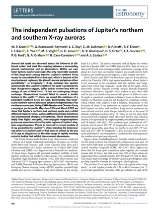
  • 2. © 2017 Macmillan Publishers Limited, part of Springer Nature. All rights reserved. LettersNATUre ASTrOnOMY hot spots for these observations, a Fourier transform was performed on the raw unsmoothed time series to produce power spectral den- sity (PSD) plots (Fig. 3). These PSDs show that on both 24 May and 1 June 2016 the southern spot pulsed with statistically signifi- cant regular periods of 9–11 min. Both Chandra and XMM-Newton independently observed this regular 9–11 min period on 24 May. A northern 12 min periodicity in the X-ray brightness was previously observed during a magnetospheric compression3 . The recurrence of a 9–12 min and 40–45 min period2,3 across multiple observations may suggest bimodal regular periodicity. Surprisingly, whereas the 9–11 min southern spot period is highly statistically significant in both observations (probability of chance occurrence (PCO) 10−5 –10−7 ), the northern spot pulsations show no significant 11 min period on 24 May and only a low-signif- icance 12-min period (PCO 10−2 ) on 1 June. The north does exhibit some lower-significance (PCO <​ 10−4 ) 5–8 min periods, but these are not consistent across hemispheres or instruments. The periodicity is not the only characteristic that seems to behave independently for each spot during these observations. The light- curves (Fig. 2) show that the brightnesses of the two spots are also uncorrelated. We observed 78 ±​ 9 X-ray photons from the southern spot during the first Chandra X-ray Observatory (CXO) observa- tion and 111 ±​ 11 X-ray photons during the second observation — a ~40% increase in X-ray emission. In contrast, we observed 298 ±​ 17 X-rays from the northern spot during the first observation, but only 189 ±​ 14 X-rays during the second; that is, the emission decreased by ~40%. Analysis of the XMM-Newton EPIC spectra (Supplementary Information) shows that the dominant emissions from the north- ern and southern aurora are from precipitating ions of O7+,8+ and S6+,…,14+ and/or C5+,6+ and therefore relate to downward current regions9,10 . To identify more precisely the sources for these precip- itating ions and the associated downward currents, we use a flux equivalence mapping model12,13 to connect magnetic field lines in the ionosphere with the equatorial magnetosphere (using the north- ern Grodent anomaly12 and southern VIP414 models). Our northern distribution (Fig. 4) matches the one observed previously3,8 , with the precipitating ions originating beyond 60RJ and between 10:00 and 19:00 magnetospheric local time (MLT). The southern spot also maps beyond 60RJ, but is concentrated between 10:00 and 14:00 MLT, and it then rotates out of view before we have the opportu- nity to observe it mapping to later MLTs. If, as with the northern spot, southern X-rays continued to be triggered when the spot maps along the afternoon–dusk flank, this emission would be unobserv- able from the Earth, addressing why fewer X-rays are almost always observed from the south15 . This broader local time origin for the northern spot may also explain the distinctive temporal signatures shown in Figs. 2 and 3, as different plasma populations, physical 180° 270° X-raysper2° X-raysper2° 90° 14 12 12 10 10 8 8 6 6 270°90° 270°90° 12 10 8 6 4 2 0 4 3 2 1 0 0.525 0.500 0.475 0.450 0.425 0.400 0.375 0.625 0.600 0.575 0.550 0.525 0.500 0.475 270°90° North North South South 180° 0° 0° 0° 0° 180° 180° Fig. 1 | Polar projections of Jupiter’s northern and southern X-ray auroras. Top row: Projections centred on Jupiter’s north (left) and south (right) poles. The projections combine 11–12 h X-ray observations of Jupiter on 24 May and 1 June 2016. Colours indicate the number of X-rays observed with the Chandra HRC in bins of 1.5° by 1.5° of S3 latitude–longitude. Dotted lines of longitude radiate from the pole, increasing clockwise (anti-clockwise) for the north (south) pole in increments of 30° from 0° at the bottom (top). Concentric dotted circles outward from the pole represent 10º increments in latitude. Thin gold contours with white text labels indicate the VIP414 model magnetic field strength in Gauss. Thick gold contours show the magnetic field ionospheric footprints of field lines intersecting the Jovigraphic equator at 5.9RJ (Io’s orbit), 15RJ and 50RJ (refs 12,13 ) from equator to pole, respectively. The location of Jupiter’s dipole magnetic pole is given by the red dot. These projections reveal that the X-ray aurora is clustered into a hot spot at both poles. The northern spot is between 155° and 180° longitude and 60° and 75° latitude, as previously observed2,3,5,7,8 . The southern spot is longitudinally broader (30°–75°) and poleward of 67° latitude, located closer to the geographic pole. Projection effects lead regions of 1.5° latitude by 1.5° longitude near the poles to appear longer in latitude than in longitude, which leads to the streak-like morphology. This is an artefact of the projection and not a physical feature. Bottom row: North (left) and south (right) polar projection exposure maps. The colour bar indicates the fraction of the total observing time during which each region was observed. These show that the clustering of X-rays in the hot spots is not due to additional observation time in these regions. Nature Astronomy | VOL 1 | NOVEMBER 2017 | 758–764 | www.nature.com/natureastronomy 759
  • 3. © 2017 Macmillan Publishers Limited, part of Springer Nature. All rights reserved. Letters NATUre ASTrOnOMY processes and/or acceleration may be involved along the dusk flank relative to the noon magnetopause. Jupiter’s magnetopause has a typical subsolar standoff distance of 60–90RJ, depending on the dynamic pressure of the solar wind16 . The flux equivalence mapping12,13 is calculated using magnetic field observations averaged over all solar wind conditions so that emis- sion mapping beyond 60RJ could indicate ions precipitating on closed field lines from the outer magnetosphere and/or field lines that are open to the solar wind, depending on solar wind conditions at the time. Of the X-rays in each spot, 30–60% of photons mapped to locations beyond the modelled expanded magnetopause location and are thus not shown on Fig. 4. Currently, the favoured explanation for the northern X-ray hot spot is that it is the signature of Jupiter’s northern cusp3,5,7,8 : that is, the dayside region of the magnetosphere that is open to the solar wind. It might therefore follow that Jupiter’s southern spot locates Jupiter’s southern cusp. For fast solar wind, X-rays are proposed to be gener- ated in this cusp region by vortical flows from pulsed reconnection at the dayside magnetopause9 . These flows change the downward cur- rents into the ionosphere and produce field-aligned potential drops of the order of megavolts9,10 . These potential drops can accelerate ~2 keV O2+ ions17 in the outer magnetosphere to the 16–32 MeV (1–2 MeV per atomic mass unit, amu) needed for Jupiter’s atmo- sphere to strip electrons and produce the observed O6+ X-ray K-shell line emissions4,6,9 . If reconnection pulses occur at Jupiter’s Alfvén- wave transit timescale of about 30–50 min, it is suggested that this mechanism could also explain the 45 min X-ray periodicity9 . However, a varied set of challenges needs to be overcome in order for pulsed dayside reconnection to explain the generation of Jupiter’s X-ray hot spots in the observation reported here: (1) the 9–12 min periodicity observed is on a shorter timescale than predicted; (2) for subsolar point reconnection, both poles should pulse periodically in-phase9 , but the dominant periodicity in the south does not also dominate the northern lightcurves (Fig. 3) and north–south pulsa- tions often appear to be independent of one another (Fig. 2); (3) the overall brightness of the northern spot seems to be uncorrelated to the overall brightness of the southern spot; and (4) a more general challenge to the proposed pulsed reconnection mechanism is that it explains X-ray emissions during fast solar wind conditions, but previously X-rays have also been observed during slow solar wind conditions3,8 . To address these challenges, here we propose adapta- tions and alternative mechanisms to explain the observed soft X-ray hot spot emissions during these observations. Differing pulsation periods for each pole could be produced by orientations of the interplanetary magnetic field that do not favour subsolar reconnection9 . At Saturn, tension associated with east–west motion of field lines during off-equatorial reconnection can produce transient non-conjugate enhancements in ultraviolet polar auroral brightness by disrupting field-aligned currents in the respective poles18 . High-latitude antiparallel reconnection may also provide non- conjugacy. Lobe reconnection has been debated19,20 as Jupiter’s 24 May 2016 CML (°) 40 North South North South 60 50 40 30 Countsperks 20 10 0 350 400 450 500 Time (min) 550 650600 70 100 130 160 190 220 1 June 2016 CML (°) 40 60 50 40 30 Countsperks 20 10 0 50 100 150 200 250 300 350 Time (min) 70 100 130 160 190 220 Fig. 2 | X-ray aurora lightcurves. Chandra X-ray lightcurves from times when the northern (blue) and southern (gold) hot spots were both observable on 24 May 2016 (top) and 1 June 2016 (bottom). The visibility as a fraction of maximum visibility for the northern (blue) and southern (gold) hot spots is indicated by the dashed curves. CML is indicated across the top, and minutes from the observation start times (10:23 and 11:32 ut, respectively) are indicated on the bottom axis. The lightcurves are one- minute binned, with six-minute moving-average smoothing. 24 May CXO southern hot spot 5 Period (min) 0 5 10 15 20 PSD 25 30 35 10–7 10–6 10–5 10–4 10–3 10–2 10–1 10 50 100 24 May CXO northern hot spot 5 Period (min) 0 5 10 15 20 PSD 25 30 35 10–7 10–6 10–5 10–4 10–3 10–2 10–1 10 50 100 1 June CXO southern hot spot 5 Period (min) 0 5 10 15 20 PSD 25 30 35 10–7 10–6 10–5 10–4 10–3 10–2 10–1 10 50 100 1 June CXO northern hot spot 5 Period (min) 0 5 10 15 20 PSD 25 30 35 10–7 10–6 10–5 10–4 10–3 10–2 10–1 10 50 100 24 May XMM southern hot spot 5 Period (min) 0 5 10 15 20 PSD 25 30 35 10–7 10–6 10–5 10–4 10–3 10–2 10–1 10 50 100 24 May XMM northern hot spot 5 Period (min) 0 5 10 15 20 PSD 25 30 35 10–7 10–6 10–5 10–4 10–3 10–2 10–1 10 50 100 Fig. 3 | X-ray aurora periodograms. PSD plots from fast Fourier transforms of X-ray lightcurves from the southern (left) and northern (right) X-ray hot spots in 2016. PSDs are shown from Chandra observations on 24 May (top), simultaneous XMM-Newton observations on 24 May (middle) and from Chandra observations on 1 June (bottom). The dotted horizontal lines show single-frequency PCO for the detected periods43 . The lowest statistical significance and highest PCO of 10−1 is at the bottom of the plot. The dashed red lines show the value obtained if photons from a steady source were randomly distributed over the visibility period. Lightcurves were extracted from 20–70° longitude and poleward of −​60° latitude for the south and from 155–180° longitude and poleward of 60° latitude for the northern hot spot. For XMM, with poorer spatial resolution and therefore subject to increased contamination from the disk emission, the lightcurves are extracted from the same time window as the Chandra observations. Nature Astronomy | VOL 1 | NOVEMBER 2017 | 758–764 | www.nature.com/natureastronomy760
  • 4. © 2017 Macmillan Publishers Limited, part of Springer Nature. All rights reserved. LettersNATUre ASTrOnOMY dominant solar-wind reconnection process. This is predominantly because the planet’s immense size, rapid rotation and internal plasma source lead to long relative timescales for return flows from an Earth-like Dungey cycle, and, under certain conditions, suppress dayside reconnection21 . For high-latitude reconnection, recon- nected/closing lobe field lines may travel equatorward across the cusp and into the dayside magnetosphere22,23 . This could explain the large spatial extent of the X-ray spots. Asymmetric high-latitude reconnection can also produce a persistent reconnection site over one pole and a moving reconnection site over the other pole. This may explain the contrasting regular 9–11 min X-ray period in the south and irregular pulsations in the north. Subsolar dayside recon- nection can produce X-rays from high-charge-state magnetosheath or solar wind ions (such as O7+ ) on open field lines, but these emis- sions are calculated to be orders of magnitude fainter than the total X-ray brightness observed9,10 . However, certain topologies of high- latitude reconnection may offer additional acceleration mecha- nisms, closing and dipolaring of stretched and/or twisted open field lines or lobe field lines in the outer magnetosphere could energize ions through Fermi acceleration. Kelvin Helmholtz instabilities (KHIs) are perhaps one of the most important large-scale instabilities that occur in coronal, mag- netospheric and astrophysical environments, transferring large quantities of energy, momentum and plasma between separate plasma regimes. They are also thought to occur at Jupiter’s mag- netopause21,24 , and they offer an alternative mechanism capable of explaining the periodic X-ray signatures3,8 . For the Earth’s magne- tosphere, KHIs can trigger magnetopause fluctuations and excite compressional ultralow-frequency (ULF) magnetic field oscilla- tions and field line resonances, driving standing Alfvén waves in the ionosphere25,26 . At Jupiter, ULF waves have been observed with 10–20 min periodicity27,28 , the lower bound of which matches our 9–12 min X-ray pulsations. The periodicity of ULF oscillations depends on the magnitude of the magnetospheric cavity, veloc- ity shear and thickness of the interaction boundary. At Jupiter, the size of the magnetosphere varies bimodally between compressed and expanded states (respective standoff distances16 63-92RJ). This could explain the bimodal 9–12 min and 40–45 min X-ray aurora periodicity. If the thickness of the magnetopause boundary, size of the magnetosphere and velocity shear were similar on 24 May and 1 June, then KHI-driven Alfvén waves could produce recurring periodicity. Moreover, KHIs could generate different brightening in each pole by driving oppositely directed field-aligned currents in each hemisphere through Ampere’s law. Traditional KHI studies focus solely on the shear in the flow as the generation mechanism. However, magnetic field orientation, plasma characteristics and thickness of the magnetopause boundary all have critical roles to play in generating wave modes along the boundary. It is for these reasons that, contrary to expectations from planetary rotation, KHIs are often observed along the dusk flank of the magnetospheres of both Earth29 and Saturn30 , as well as the dawn sector, where the velocity shear is largest. Indeed, at larger velocity shears, KHI may also be stabilized30 . The prevalence and locations of KHIs, alongside the possibility of KHI-generated acceleration of the order of the MeV amu-1 required for the observed X-ray signatures, remain to be fully explored at Jupiter. However, wave–particle inter- actions, KHI-driven reconnection and/or modulation of current systems and their associated potential drops are all possible accel- eration mechanisms. The southern X-ray spot rotates out of view while the northern spot rotates into view, so that they are observable simultaneously only when they approach opposite limbs of Jupiter’s observable disk. If the two spots are globally driven, then arguably the simplest explanation for the north–south differences is that magnetospheric conditions changed with time and damped the 11 min southern period. Whether the differences are due to changes with time or North spot X-ray South spot X-ray Noon 100 100 50 50 B J 0 0 –50 –50 x (RJ) y(RJ) –100 –100 Dawn Dusk Fig. 4 | Ionosphere–magnetosphere mapping for the X-ray hot spots with accompanying schematic for a KHI driver. Top: Mapping13 of X-ray photon emission located in the ionosphere to the equatorial magnetosphere source regions for the northern (blue) and southern (gold) hot spots. The solid red lines indicate Jupiter’s magnetopause, for an expanded 92RJ, standoff distance (outer contour) and compressed 63RJ standoff distance (inner contour)16 . We also note that even for the statistical location of the expanded magnetopause, because of the substantial spatial extent of the hot spots, 30–60% of X-rays mapped beyond the magnetopause, meaning that their origins cannot be identified by the model mapping, and they are not plotted here. Bottom: Illustration of a possible source mechanism for the observed hot spot emissions. KHIs along the magnetopause could produce field line resonances that generate regular periodicity in the emissions. Further, these field line resonances could vary bimodally with the compressed or expanded states of Jupiter’s magnetosphere. These KHIs may also generate non-conjugate north–south auroral signatures, as twisting of the magnetic field line (illustrated in red, B) can generate inter-hemispheric currents (green, J). Schematics for drivers relating to field line tension from the Y-component of the Interplanetary Magnetic Field (IMF) or high latitude reconnection can be found in ref. 18 and ref. 23 respectively. Nature Astronomy | VOL 1 | NOVEMBER 2017 | 758–764 | www.nature.com/natureastronomy 761
  • 5. © 2017 Macmillan Publishers Limited, part of Springer Nature. All rights reserved. Letters NATUre ASTrOnOMY due to differing polar dynamics, both auroral spots are fixed in the planet’s rotating coordinate system, so localized magnetic condi- tions may also play some part in ensuring that ion acceleration to energies of the order of MeV amu–1 is produced only in the hot spots and not in any other auroral region. These findings also highlight possible multi-wavelength con- nections for Jupiter’s aurora. Ultraviolet polar auroral flares31 sometimes coincide with X-ray brightenings5 and, like the X-ray pulsations, quasi-periodically enhance on roughly a 10 min tim- escale32 . Bright infrared auroral hot spots are also co-located with the X-ray hot spots, which may suggest that the pulses of precipita- tion of high-energy ions, and their associated drivers, provide an important heating mechanism for Jupiter’s stratosphere down to the 10 mbar pressure level33 . The independent behaviour of Jupiter’s pair of soft X-ray hot spots during these observations raises fundamental questions about what processes at rapidly rotating magnetospheres produce these auroras. For Jupiter, the spectral signatures of the precipitating ions suggest that the spots locate Jupiter’s downward currents10 and may identify the northern and southern cusps9 . However, the observed distinctive behaviour could be indicative of non-equatorial recon- nection, magnetopause-driven ULF waves, tail reconnection or local magnetic conditions at each polar region. Over the coming 2 years, X-ray observing campaigns in conjunction with NASA’s Juno mission will offer the opportunity to determine whether the independent behaviour that we report here is commonplace or is unique to the observations presented here. Critically, they will help to identify the magnetospheric conditions and auroral processes that are able to generate Jupiter’s highest-energy emissions and the seemingly independent behaviour of the northern and southern soft X-ray hot spots. Method Observation times. For all previously published X-ray campaigns with Chandra2,3,5,7,8 and XMM-Newton (XMM)4,8,34,35 , the viewing geometry favoured observations of the northern aurora. At these times, the sub-Earth latitudes of 0.2°–3.9° and north pole distance angles of 18°–23° obscured visibility of the geographic south pole (Supplementary Material). However, during summer 2016 and March 2007, the tilt of Jupiter relative to the X-ray instruments in Earth orbit allowed clear X-ray observations of Jupiter’s southern geographic pole (north pole angle of −​17° and −​16° respectively and sub-Earth latitude of −​1.7° and −​3.3° respectively). It is this viewing geometry, which is rare in the legacy X-ray observations of Jupiter (see Supplementary Materials), that permitted clear observations of the southern X-ray hot spot. The 2016 Chandra observations and XMM observation continuously observed a total CML range of 425° and 482° respectively during the 11.7 h Chandra observations (1.17 Jupiter rotations) and 12.3 h XMM observation (1.23 Jupiter rotations). The Chandra observations on 24 May and 1 June started with a CML of 185° and 350° respectively and finished with a CML of 250° and 55° respectively. The XMM-Newton observation on 24 May started with a CML of 175° and finished with a CML of 297°.The Chandra ACIS 5 h observation on 3 March 2007 covered a CML range of 290°–110°. The entirety of Jupiter’s disk fits within the field of view of both Chandra HRC and ACIS instruments and XMM- Newton’s EPIC-PN instrument, permitting simultaneous observations of Jupiter’s northern and southern hot spots during the CML window when both spots are at least partially on the observed disk. However, we note that the southern spot is rotating out of view when the Northern spot rotates into view, so that both spots can only be simultaneously observed in their entirety between CMLs ~90°–120°, and at these times there are still viewing geometry limitations and possible effects produced by the viewing angle of precipitation and/or the angle at which the X-rays are emitted. Given that each observation continuously covered 1.2 Jupiter rotations, this meant that, for both observations, Jupiter’s northern and southern hot spots were observed at least once, and the 24 May (1 June) observation partially observed Jupiter’s northern (southern) hot spot a second time. To ensure that we did not artificially enhance the X-ray counts by including multiple visits to the same spot (two visits to the north on 24 May and two to the south on 1 June), in each observation we extracted counts only from the longest duration window of these two possible observing windows. A table of the counts recorded by Chandra from every observing window can be found in the Supplementary Information. Supplementary Fig. 1 shows a projection onto the south pole from the Chandra ACIS observation on 3 March 2007. To analyse the ACIS data, we applied a correction to the effective area3,5 to account for the increased energy thresholds applied within ACIS to circumvent optical light leaks through the optical blocking filters. This observation had a lower observer co-latitude (Supplementary Table 1), offering better visibility of the geographic south pole than the 2016 campaign. Although the observations from the 2007 campaign were dimmer than those from 2016 and used a different instrument (Chandra ACIS instead of Chandra HRC), the polar projection shows that the X-rays are again concentrated into the southern hot spot and that this occurs from 70° latitude to the pole and between 30°–60° S3 longitude. Studies of eight X-ray observations of the northern spot have shown that, from observation to observation, the hot spot expands and contracts centred on a persistent location3,8 . This may suggest that although the southern spot is centred on the same location in 2007 and 2016, it also expands and contracts from this location. Alternatively, the apparent expansion in the 2016 observations may be a projection effect produced by the slightly poorer visibility of the region during the 2016 observations relative to the 2007 observations. Supplementary Fig. 2 quantifies the concentrations of X-rays shown in Fig. 1 and Supplementary Fig. 1. In the 2016 and 2007 observations, the southern hot spot occurred in the same longitude range, suggesting that it is a persistent feature of the southern X-ray aurora. We contrast the count concentrations in the auroral zones with emission from fluoresced and scattered solar photons in Jupiter’s equatorial atmosphere. This demonstrates that the distributions are not produced by transient variations in the solar X-ray flux. If this were the case, then the disk distributions might be expected to match the auroral distributions, and they do not. We also plot error bars on the count measurements, highlighting the significance of the spots’ longitudinal concentrations relative to the more uniform equatorial emission. Spectral analysis. We analysed the XMM-Newton EPIC-PN spectral data from 24 May to identify the source populations of the observed emissions. To do this, we applied the standard high-energy astrophysics software packages including XMM-SAS and XSPEC. XMM-Newton has lower spatial resolution than Chandra. To circumvent this, we used the information from Chandra (from the overlapping interval) on the spatial locations of the spots with visibility information from NASA JPL Horizons ephemerides data to select times that corresponded to CML ranges when the hot spots were on Jupiter’s observable disk. For XMM, for the north (south) we extracted hot spot spectra from times when the CML ranges were 60°–270° (300°–170°). The time intervals outside these windows were checked to ensure that the X-ray emission was evenly distributed across Jupiter’s entire disk and no significant auroral concentrations were lost. Given the dynamic nature of the hot spots, we only used the longest observation window and did not combine the shorter partial observation windows with this. This disregarding of times when the hot spot was unobservable is an alteration from previous spectral studies34,36 ; it allowed us to minimize contamination from scattered solar photons and provided a more accurate calculation of X-ray emission rates from the aurora only. Using the standard XMM-SAS package, we then selected the appropriate source regions for the northern and southern aurora from a planet-centred image and extracted the relevant spectral products (spectral data from source region, spectral data from background region, effective area/auxiliary response and redistribution matrix files). To ensure that there were sufficient counts to reliably fit models, we binned the data into 10-channel energy bins. Using the XSPEC modelling package, we then tested model fits for a combination of different Gaussian lines and bremsstrahlung continuum to a non-background-subtracted spectrum (Jupiter’s disk blocks cosmic X-ray background emission5 ). To distinguish between auroral emission and potential contamination in the polar region from fluorescence or scattering of solar photons in Jupiter’s atmosphere, we also extracted the equatorial emission by using the same time window as the auroral emissions. Given the low count rates, we used an equatorial spectrum that covered the times when either hot spot was observable (sub- observer longitude 300°–270°). Modelling of the equatorial spectrum showed clearly distinctive features from the auroral emissions, indicating that the auroral spectra were dominated by a different emission process (that is, not fluorescence and scattering of solar photons). A bremsstrahlung continuum was found not to give good fits for the northern or southern auroral emissions, suggesting that both observed hot spots are dominated by spectral lines from precipitating ions. It was challenging to compare the northern and southern auroras directly because of the low count levels for the south, but both the north (Supplementary Table 6) and south (Supplementary Table 7) best-fit models feature a prominent and well-defined O vii line centred on 568 eV and a high flux line in the region where a range of sulfur and carbon lines are present. Both aurora best-fit models also include a line at 430–470 eV where there are known C vi lines. Interestingly, carbon is much more abundant in the solar wind than in Jupiter’s magnetosphere, so this could suggest some direct solar wind precipitation. However, we note that the 90% confidence errors on the fluxes for this specific line are 50% of the measured flux for the north and more than this for the south. This 430–470 eV line coincides with the lowest data point between 200 and 900 eV on the equatorial spectrum, suggesting that it is not contamination from scattered solar photons, but is a part of the auroral spectrum. The equatorial spectrum (Supplementary Fig. 5) Nature Astronomy | VOL 1 | NOVEMBER 2017 | 758–764 | www.nature.com/natureastronomy762
  • 6. © 2017 Macmillan Publishers Limited, part of Springer Nature. All rights reserved. LettersNATUre ASTrOnOMY does hint at the presence of a line at 400 eV, and we attempted to force model fits to this, but these always led to worse fits and increased the reduced χ2 by at least 0.5. As with previous Jovian disk analysis37 , we could attain a good fit (reduced χ2 of ~0.7) to the equatorial spectrum from 500–1,500 eV with a vmekal hot plasma model using solar abundances with kT ≈​ 0.3 and flux of ~9 ×​ 10−7 photons cm−2  s−1 . To support comparison with the auroral emission (Supplementary Fig. 5), we show a spectral model fitted with known solar spectrum lines38 : this shows that the equatorial emission has a very different structure above 600 eV. If the observed and modelled auroral emissions were due to solar contamination, then one would not expect the auroral emissions to decrease above 600 eV, as they do. Given that both the northern and southern auroras feature similar O vii, sulfur and carbon lines, this may support a similar source population (as suggested by the magnetospheric mapping to the noon magnetopause). This may also suggest that any independent behaviour is locally driven. The northern aurora is better fitted with the inclusion of an O viii line. More energy is required to strip the additional electron in order to produce this line, so the presence of the extra line may hint that a more energetic pulsation process occurs in the observable northern aurora than in the south. This higher-charge- state oxygen would, through charge exchange, subsequently lead to a cascade of emissions from oxygen in lower charge states, which may explain further differences between the oxygen spectra. We note that the source regions for the two spectra are different (see Fig. 4), which may explain some of the spectral differences (there may be changes in acceleration, the driver process or the source ion population when moving from the nose to the dusk flank), and the spectra do not cover the same time interval. However, from this single north–south spectral comparison, it is difficult to quantify the differences between the two spectra conclusively, as the intensities of the southern spectral lines are a factor of 2–4 lower than for the north. Future observations that provide good visibility of both poles will help to address and interpret the spectral characteristics with more statistical certainty. Lightcurves and XMM-Newton periodicity detection. For Chandra, the 1-min-binned lightcurves (Supplementary Fig. 2) from the northern spot were produced by extracting X-rays from 155°–190° longitude and poleward of 60° latitude. For the south, the 1-min-binned lightcurves (Supplementary Fig. 2) were extracted from 20°–70° longitude and poleward of −​60° latitude. The 1-min-binned unsmoothed data were then fast Fourier transformed to produce the PSDs shown in Fig. 4 of the main text. The lightcurves shown in Fig. 3 and Supplementary Figs. 3 and 4 have been smoothed with a 6 minute moving average. As with previous work2,3,5 , no moving-average smoothing was applied to generate the Fourier transform frequency data. Supplementary Fig. 3 shows the complete northern and southern auroral lightcurves for 24 May (Chandra and XMM- Newton) and 1 June (Chandra) 2016. The lightcurves from XMM-Newton’s EPIC contain more noise than the Chandra HRC lightcurves because EPIC’s lower spatial resolution leads to additional contamination from fluoresced and scattered solar X-ray photons on Jupiter’s disk. This limited spatial resolution also prevents lightcurves from being extracted based on S3 coordinate locations. As with the spectra, we therefore extracted XMM-Newton auroral lightcurves from the auroral region, during the same time window as the spectra — times when longitudes connected to the X-ray hot spots were observable (CML 60°–270° or 300°–170° for the northern and southern aurora respectively). The XMM-Newton southern (northern) PSDs shown in Fig. 4 were therefore produced from Fourier transforms of the 300–500 min (450–700 min) unsmoothed data that generated these lightcurves. The lightcurves for XMM-Newton are noisier, as the spatial resolution is not as good as Chandra’s, and it was therefore not possible to select areas in S3 coordinates. Instead, we used auroral regions extracted from the disk of Jupiter, which will include additional contamination from the disk emission. There are also different energy-dependent responses and effective areas for XMM-Newton’s EPIC and Chandra’s HRC and ACIS instruments, which may lead to differing lightcurve morphology for each instrument. Jupiter’s equatorial emissions are produced by solar photons that are fluoresced and scattered in Jupiter’s atmosphere37,39,40 . Lightcurves and PSDs from the Jovian equator on 24 May (day of year (DoY) 145) and 1 June (DoY 153) (Supplementary Fig. 4) between −​30° and 30° latitude demonstrate that the periodic behaviour is not present in the equatorial region and that there was not a significant variation in the solar X-ray output (for example from solar flares) during the observations3,37,40 . To statistically test how similar the PSDs were between each pole, each instrument and each observation, we conducted a range of hypothesis tests and calculated the P-value41 for each compared data set. Direct comparisons of a hot spot PSD from the same pole but in different observations or instruments produced relatively high P-values (Supplementary Table 4), suggesting that the temporal behaviours of the emissions were similar. However, directly comparing the northern PSDs with the southern PSDs produced low P-values, suggesting the inter-hemisphere temporal behaviour is far less similar. Supplementary Table 5 shows results from statistical analyses using the STA/ LTA algorithm42 to identify and characterize the three most prominent peaks in the PSD plots in Fig. 4. This auto-detection of the peaks in the periodogram quantifies and characterizes the strong 9–11 min period observed in the southern spot, which is not also observed in the northern spot. We note, however, that a 5–8 min period does seem to recur in the north. Data availability. The data analysed within this paper are publicly available from the Chandra and XMM-Newton Data Archives. Received: 3 February 2017; Accepted: 25 August 2017; Published online: 30 October 2017 References 1. Hallinan, G. et al. Magnetospherically driven optical and radio aurorae at the end of the stellar main sequence. Nature 523, 568–571 (2015). 2. Gladstone, G. R. et al. A pulsating auroral X-ray hot spot on Jupiter. Nature 415, 1000–1003 (2002). 3. Dunn, W. R. et al. The impact of an ICME on the Jovian X-ray aurora. J. Geophys. Res. A Space Phys. 121, 2274–2307 (2016). 4. Branduardi-Raymont, G. et al. A study of Jupiter’s aurorae with XMM-Newton. Astron. Astrophys. 463, 761–774 (2007). 5. Elsner, R. F. et al. Simultaneous Chandra X ray Hubble Space Telescope ultraviolet, and Ulysses radio observations of Jupiter’s aurora. J. Geophys. Res. Space Phys. 110, 1–16 (2005). 6. Kharchenko, V., Bhardwaj, A., Dalgarno, A., Schultz, D. R. & Stancil, P. C. Modeling spectra of the north and south Jovian X-ray auroras. J. Geophys. Res. Space Phys. 113, 1–11 (2008). 7. Branduardi-Raymont, G. et al. Spectral morphology of the X-ray emission from Jupiter’s aurorae. J. Geophys. Res. Space Phys. 113, 1–11 (2008). 8. Kimura, T. et al. Jupiter’s X-ray and EUV auroras monitored by Chandra, XMM-Newton, and Hisaki satellite. J. Geophys. Res. Space Phys. 121, 2308–2320 (2016). 9. Bunce, E. J., Cowley, S. W. H. & Yeoman, T. K. Jovian cusp processes: Implications for the polar aurora. J. Geophys. Res. Space Phys. 109, 1–26 (2004). 10. Cravens, T. E. et al. Implications of Jovian X-ray emission for magnetosphere- ionosphere coupling. J. Geophys. Res. Space Phys. 108, 1–12 (2003). 11. Cowley, S. W. H. & Bunce, E. J. Origin of the main auroral oval in Jupiter’s coupled magnetosphere-ionosphere system. Planet. Space Sci. 49, 1067–1088 (2001). 12. Grodent, D. et al. Auroral evidence of a localized magnetic anomaly in Jupiter’s northern hemisphere. J. Geophys. Res. Space Phys. 113, 1–10 (2008). 13. Vogt, M. F. et al. Improved mapping of Jupiter’s auroral features to magnetospheric sources. J. Geophys. Res. Space Phys. 116, 1–24 (2011). 14. Connerney, J. E. P., Acuña, M. H., Ness, N. F. & Satoh, T. New models of Jupiter’s magnetic field constrained by the Io flux tube footprint. J. Geophys. Res. 103, 11929–11939 (1998). 15. Waite, J. H. et al. ROSAT observations of the Jupiter aurora. J. Geophys. Res. 99, 799–809 (1994). 16. Joy, S. P. et al. Probabilistic models of the Jovian magnetopause and bow shock locations. J. Geophys. Res. Space Phys. 107, 1–17 (2002). 17. Bagenal, F. Empirical model of the Io plasma torus: Voyager measurements. J. Geophys. Res. 99, 11043 (1994). 18. Meredith, C. J., Cowley, S. W. H., Hansen, K. C., Nichols, J. D. & Yeoman, T. K. Simultaneous conjugate observations of small-scale structures in Saturn’s dayside ultraviolet auroras: implications for physical origins. J. Geophys. Res. Space Phys. 118, 2244–2266 (2013). 19. McComas, D. J. & Bagenal, F. Jupiter: a fundamentally different magnetospheric interaction with the solar wind. Geophys. Res. Lett. 34, 1–5 (2007). 20. Cowley, S. W. H., Badman, S. V., Imber, S. M. & Milan, S. E. Comment on ‘Jupiter: a fundamentally different magnetospheric interaction with the solar wind’ by D. J. McComas and F. Bagenal. Geophys. Res. Lett. 35, 1–3 (2008). 21. Desroche, M., Bagenal, F., Delamere, P. A. & Erkaev, N. Conditions at the expanded Jovian magnetopause and implications for the solar wind interaction. J. Geophys. Res. Space Phys. 117, 1–18 (2012). 22. Lockwood, M. & Moen, J. Reconfiguration and closure of lobe flux by reconnection during northward IMF: possible evidence for signatures in cusp/cleft auroral emissions. Ann. Geophys. 17, 996–1011 (1999). 23. Fuselier, S. A., Trattner, K. J., Petrinec, S. M. & Lavraud, B. Dayside magnetic topology at the Earth’s magnetopause for northward IMF. J. Geophys. Res. Space Phys. 117, 1–14 (2012). 24. Delamere, P. A. & Bagenal, F. Solar wind interaction with Jupiter’s magnetosphere. J. Geophys. Res. Space Phys. 115, 1–20 (2010). 25. Mann, I. R. et al. Coordinated ground-based and Cluster observations of large amplitude global magnetospheric oscillations during a fast solar wind speed interval. Ann. Geophys. 20, 405–426 (2002). 26. Rae, I. J. et al. Evolution and characteristics of global Pc5 ULF waves during a high solar wind speed interval. J. Geophys. Res. Space Phys. 110, 1–16 (2005). 27. Khurana, K. K. & Kivelson, M. G. Ultralow frequency MHD waves in Jupiter’s middle magnetosphere. J. Geophys. Res. 94, 5241 (1989). Nature Astronomy | VOL 1 | NOVEMBER 2017 | 758–764 | www.nature.com/natureastronomy 763
  • 7. © 2017 Macmillan Publishers Limited, part of Springer Nature. All rights reserved. Letters NATUre ASTrOnOMY 28. Wilson, R. J. & Dougherty, M. K. Evidence provided by galileo of ultra low frequency waves within Jupiter’s middle magnetosphere. Geophys. Res. Lett. 27, 835–838 (2000). 29. Hasegawa, H. et al. Transport of solar wind into Earth’s magnetosphere through rolled-up Kelvin–Helmholtz vortices. Nature 430, 755–758 (2004). 30. Ma, X., Stauffer, B., Delamere, P. A. & Otto, A. Asymmetric Kelvin– Helmholtz propagation at Saturn’s dayside magnetopause. J. Geophys. Res. Space Phys. 120, 1867–1875 (2015). 31. Bonfond, B. et al. Quasi-periodic polar flares at Jupiter: a signature of pulsed dayside reconnections? Geophys. Res. Lett. 38, 1–5 (2011). 32. Nichols, J. D. et al. Response of Jupiter’s auroras to conditions in the interplanetary medium as measured by the Hubble Space Telescope and Juno. Geophys. Res. Lett. 44, 7643–7652 (2017). 33. Sinclair, J. A. et al. Independent evolution of stratospheric temperatures in Jupiter’s northern and southern auroral regions from 2014 to 2016. Geophys. Res. Lett. 44, 5345–5354 (2017). 34. Branduardi-Raymont, G., Elsner, R. F., Gladstone, G. R. & Ramsay, G. First observation of Jupiter by XMM-Newton. Astron. Astrophys. 337, 331–337 (2004). 35. Hui, Y. et al. Comparative analysis and variability of the Jovian X-ray spectra detected by the Chandra and XMM-Newton observatories. J. Geophys. Res. Space Phys. 115, A07102 (2010). 36. Branduardi-raymont, G. et al. Thermal and non-thermal components of the X-ray emission from Jupiter. Progr. Theor. Exp. Phys. 169, 75–78 (2007). 37. Branduardi-Raymont, G. et al. Latest results on Jovian disk X-rays from XMM-Newton. Planet. Space Sci. 55, 1126–1134 (2007). 38. Phillips, K. J. H. et al. Solar flare X-ray spectra from the Solar Maximum Mission Flat Crystal Spectrometer. Astrophys. J. 256, 774–787 (1982). 39. Bhardwaj, A. et al. Solar control on Jupiter’s equatorial X-ray emissions: 26–29 November 2003 XMM-Newton observation. Geophys. Res. Lett. 32, 1–5 (2005). 40. Bhardwaj, A. et al. Low- to middle-latitude X-ray emission from Jupiter. J. Geophys. Res. Space Phys. 111, 1–16 (2006). 41. Selke, T., Bayarri, J. J. & Berger, J. O. Calibration of p-values for testing precise hypotheses. Am. Stat. 55, 62–71 (2001). 42. Allen, R. Automatic phase pickers: their present use and future prospects. Bull. Seismol. Soc. Am. 72, S225–242 (1982). 43. Leahy, D. A. et al. On searches for pulsed emission with application to four globular cluster X-ray sources—NGC 1851, 6441, 6624, and 6712. Astrophys. J. 266, 160–170 (1983). Acknowledgements W.R.D. thanks N. Achilleos and R. Gray for discussions on Jovian X-rays, J.-U. Ness and R. Gonzalez-Riestra for extensive help with XMM-Newton observations, and particularly P. Rodriguez for assistance in re-framing them to Jupiter-centred coordinates. We also thank S. Badman, B. Bonfond, E. Chané, G. Clark, P. Delamere, R. Ebert, H. Hasegawa, S. Imber, E. Kronberg, P. Lourn, W. Kurth, A. Masters, J. Nichols, A. Otto, C. Paranicas, A. Radioti, J. Reed, E. Roussos, A. Smith and C. Tao for conversations on Jupiter’s aurora at the Vogt/Masters and Jackman/Paranicas ISSI team meetings. W.R.D. is supported by a Science and Technology Facilities Council (STFC) research grant to University College London (UCL), an SAO fellowship to Harvard-Smithsonian Centre for Astrophysics and by European Space Agency (ESA) contract no. 4000120752/17/NL/MH. I.J.R., G.H.J., G.B.-R. and A.J.C. are supported by STFC Consolidated Grant ST/N000722/1 to the Mullard Space Science Laboratory (MSSL). I.J.R. is supported by NERC grants NE/ L007495/1, NE/P017150/1 and NE/P017185/1. G.A.G. is supported by a UCL IMPACT studentship and ESA. C.M.J. is supported by a STFC Ernest Rutherford Fellowship ST/ L004399/1. M.F.V. is supported by the US National Science Foundation under Award No. 1524651. Z.Y. is a Marie-Curie COFUND postdoctoral fellow at the University of Liege, co-funded by the European Union. G.R.G. thanks Smithsonian Astrophysical Observatory for award GO6-17001A to the Southwest Research Institute. J.A.S. and G.S.O. acknowledge support from NASA to the Jet Propulsion Laboratory, California Institute of Technology. R.C.-C. acknowledges support from Universidad Pontificia Comillas de Madrid-ICAI and Universidad Complutense de Madrid-Facultad de Informática This work is based on observations from the NASA Chandra X-ray Observatory (Observations 18608, 18609 and archival observation 8219) made possible through the HRC grant (NAS8-03060) and observations from the XMM-Newton Observatory (Observations 0781830301 and 0781830601). We thank the Chandra and XMM-Newton Projects for their support in setting up the observations Author contributions All authors were involved in the writing of the paper. W.R.D. led the work, organized the XMM-Newton observations and conducted most of the analysis for both CXO and XMM-Newton data sets. G.B.-R. provided expertise on XMM-Newton and analysis for the XMM-Newton data. L.C.R. provided knowledge of planetary magnetospheric dynamics and critical review of the techniques applied, along with extensive paper writing and code to support the analysis. C.M.J. and R.P.K. organized the Chandra observations and reviewed the Chandra data analysis. R.F.E. provided essential and invaluable analysis tools for the CXO data. I.J.R. and Z.Y. provided expertise on auroral drivers, magnetospheric processes and periodicity, and wrote several paragraphs of the paper. M.F.V. provided model mapping to identify origins for the auroral emissions. G.R.G. provided expertise on the Jovian auroral emissions and was Principal Investigator of the 2007 Chandra observation reported here. G.H.J. provided the sketch of the KHI mechanism that could produce the non-conjugacy observed in the emissions. G.S.O. and J.A.S. triggered the initial analysis through discussions and critical review combining infrared and X-ray emissions from the south pole. P.G.F. provided code to reduce data from CXO given ACIS instrument degradation. G.A.G. provided code to support mapping of emissions. R.C.-C. provided statistical analysis tools for the timings. A.J.C. provided detailed knowledge of planetary magnetospheres. Competing interests The authors declare no competing financial interests. Additional information Supplementary information is available for this paper at https://doi.org/10.1038/s41550- 017-0262-6. Reprints and permissions information is available at www.nature.com/reprints. Correspondence and requests for materials should be addressed to W.R.D. Publisher’s note: Springer Nature remains neutral with regard to jurisdictional claims in published maps and institutional affiliations. Nature Astronomy | VOL 1 | NOVEMBER 2017 | 758–764 | www.nature.com/natureastronomy764