SlideShare una empresa de Scribd logo
1 de 40
Introduction to Calculus
Calculus is all about changes.
Sam and Alex are travelling in the car ... but the
speedometer is broken.
Alex: "Hey Sam! How fast are we going now?"
Sam: "Wait a minute ..."
"Well in the last minute we went 1.2 km, so we are going:"
1.2 km/minute x 60 minutes in an hour = 72 km/h
Alex: "No, Sam! Not our average for the last minute, or even the last second,
I want to know our speed RIGHT NOW."
Sam: "OK, let us measure it up here ... at this road sign... NOW!"
"OK, we were AT the sign for zero seconds, and the distance was
... zero meters!"
The speed is 0m / 0s = 0/0 = I Don't Know!
"I can't calculate it Sam! I need to know some distance
over some time, and you are saying the time should be zero? Can't be
done."
That is pretty amazing ... you'd think it is easy to work out the speed of a car at
any point in time, but it isn't.
Even the speedometer of a car (when it works!) just shows us an average of
how fast we were going for the last very short amount of time.
How About Getting Real Close
But our story is not finished yet!
Sam and Alex get out of the car, because they have arrived on location. Sam is
about to do a stunt:
Sam will do a jump off a 20 m building.
Alex, as photographer, asks:
"How fast will you be falling after 1 second?"
Sam uses this simplified formula to find the distance fallen:
d = 5t2
 d = distance fallen, in meters
 t = time from jump, in seconds
Example: at 1 second Sam has fallen
d = 5t2
= 5 × 12
= 5 m
But how fast is that? Speed is distance over time:
Speed =
distance
time
So at 1 second:
Speed =
5 m
= 5 m/s
1 second
"BUT", says Alex, "again that is an average speed, since you started the jump,
... I want to know the speed at exactly 1 second, so I can set up the camera
properly."
Well ... at exactly 1 second the speed is:
Speed =
5 − 5 m
=
0 m
= ????
1 − 1 s 0 s
So again Sam has a problem.
Think about it ... how do we figure out a speed at an exact instant in time?
What is the distance? What is the time difference?
They are both zero, giving us nothing to calculate with!
But Sam has an idea ... invent a time so short it won't matter.
Sam won't even give it a value, and will just call it "Δt" (called "delta t").
So Sam works out the difference in distance between t and t+Δt
At 1 second Sam has fallen
d = 5t2
= 5 × (1)2
= 5 m
At (1+Δt) seconds Sam has fallen
d = 5t2
= 5 × (1+Δt)2
m
We can expand (1+Δt)2
:
(1+Δt)2 = (1+Δt)(1+Δt)
= 1 + 2Δt + (Δt)2
And we get:
d = 5 × (1+2Δt+(Δt)2
) m
= 5 + 10Δt + 5(Δt)2
m
So between 1 second and (1+Δt) seconds the distance fallen is:
Change in d = (5 + 10Δt + 5(Δt)2
) − 5 m
= 10Δt + 5(Δt)2
m
Now divide that distance by time to get the speed:
Speed= 10Δt +5(Δt)2 mΔt s
= 10 + 5Δt m/s
So the speed is 10 + 5Δt m/s, and Sam thinks about that Δt value ... he
wants Δt to be so small it won't matter ... so he imagines it shrinking
towards zero and he gets:
Speed = 10 m/s
Wow! Sam got an answer!
Sam: "I will be falling at exactly 10 m/s"
Alex: "I thought you said you couldn't calculate it?"
Sam: "That was before I used Calculus!"
Yes, indeed, that was Calculus.
The word Calculus comes from Latin meaning "small stone".
Because it is like understanding something by looking at small pieces.
Differential Calculus cuts something into small pieces to find how it changes.
Integral Calculus joins (integrates) the small pieces together to find how
much there is.
And Differential Calculus and Integral Calculus are like inverses of each other,
just like multiplication and division are inverses.
Sam used Differential calculus to cut time and distance into such small pieces
that a pure answer came out.
So ... was Sam's result just luck? Does it work for other things?
Let's try doing this for the function y = x3
This is going to be very similar to the previous example, but it will be just a
slope on a graph, no one has to jump for this one!
Example: What is the slope of the function y = x3
at x=1 ?
At x = 1, y = 13
= 1
At x = (1+Δx), y = (1+Δx)3
We can expand (1+Δx)3
to 1 + 3Δx + 3(Δx)2
+ (Δx)3
, and we get:
y = 1 + 3Δx + 3(Δx)2
+ (Δx)3
And the difference between the y values from x = 1 to x = 1+Δx is:
Change in y = 1 + 3Δx + 3(Δx)2
+ (Δx)3
− 1
= 3Δx + 3(Δx)2
+ (Δx)3
Now we can calculate slope:
Slope = 3Δx + 3(Δx)2
+ (Δx)3
Δx
= 3 + 3Δx + (Δx)2
Once again, as Δx shrinks towards zero we are left with:
Slope = 3
And here we see the graph of y = x3
The slope is continually changing, but at the
point (1,1) we can draw a line tangent to the curve
and find the slope there really is 3.
(Count the squares if you want!)
Question for you: what is the slope at the point (2,8)?
Try It Yourself!
Go to the Slope of a Function page, put in the formula "x^3", then try to find
the slope at the point (1,1).
Zoom in closer and closer and see what value the slope is heading towards.
Conclusion
Calculus is about changes.
Differential calculus cuts something into small pieces to find how it changes.
 Learn more at Introduction to Derivatives
Integral calculus joins (integrates) the small pieces together to find how
much there is.
 Learn more at Introduction to Integration
Introduction to Derivatives
It is all about slope!
Slope = Change in YChange in X
We can find an average slope between two points.
But how do we find the slope at a point?
There is nothing to measure!
But with derivatives we use a small difference ...
... then have it shrink towards zero.
Let us Find a Derivative!
We will use the slope formula:
Slope = Change in YChange in X = ΔyΔx
to find the derivative of a function y = f(x)
x changes from x to x+Δx
y changes from f(x) to f(x+Δx)
Follow these steps:
• Fill in this slope formula: ΔyΔx = f(x+Δx) − f(x)Δx
• Simplify it as best we can,
• Then make Δx shrink towards zero.
Here we go:
Example: the function f(x) = x2
We know f(x) = x2, and can calculate f(x+Δx) :
Start with: f(x+Δx) = (x+Δx)2
Expand (x + Δx)2
: f(x+Δx) = x2
+ 2x Δx + (Δx)2
The slope formula is:
f(x+Δx) − f(x)
Δx
Put in f(x+Δx) and f(x):
x2
+ 2x Δx + (Δx)2
− x2
Δx
Simplify (x2
and −x2
cancel): =
2x Δx + (Δx)2
Δx
Simplify more (divide through by Δx): = 2x + Δx
And then as Δx heads towards 0 we get: = 2x
Result: the derivative of x2
is 2x
We write dx instead of "Δx heads towards 0", so "the derivative of" is
commonly written
x2 = 2x
"The derivative of x2 equals 2x"
or simply "d dx of x2
equals 2x"
What does x2 = 2x mean?
It means that, for the function x2
, the slope or "rate of change" at any point
is 2x.
So when x=2 the slope is 2x = 4, as shown here:
Or when x=5 the slope is 2x = 10, and so on.
Note: sometimes f’(x) is also used for "the derivative of":
f’(x) = 2x
"The derivative of f(x) equals 2x"
Let's try another example.
Example: What is x3 ?
We know f(x) = x3
, and can calculate f(x+Δx) :
Start with: f(x+Δx) = (x+Δx)3
Expand (x + Δx)3
: f(x+Δx) = x3
+ 3x2
Δx + 3x (Δx)2
+ (Δx)3
The slope formula:
f(x+Δx) − f(x)
Δx
Put in f(x+Δx) and f(x):
x3
+ 3x2
Δx + 3x (Δx)2
+ (Δx)3
− x3
Δx
Simplify (x3
and −x3
cancel): =
3x2 Δx + 3x (Δx)2 + (Δx)3
Δx
Simplify more (divide through by Δx): = 3x2
+ 3x Δx + (Δx)2
And then as Δx heads towards 0 we get: x3 = 3x2
Have a play with it using the Derivative Plotter.
Derivatives of Other Functions
We can use the same method to work out derivatives of other functions (like
sine, cosine, logarithms, etc).
But in practice the usual way to find derivatives is to use:
Derivative Rules
Example: what is the derivative of sin(x) ?
On Derivative Rules it is listed as being cos(x)
Done.
Using the rules can be tricky!
Example: what is the derivative of cos(x)sin(x) ?
You can't just find the derivative of cos(x) and multiply it by the derivative of
sin(x) ... you must use the "Product Rule" as explained on the Derivative
Rules page.
It actually works out to be cos2
(x) - sin2
(x)
So that is your next step: learn how to use the rules.
Notation
"Shrink towards zero" is actually written as a limit like this:
"The derivative of f equals the limit as Δx goes to zero of f(x+Δx) - f(x)
over Δx"
Or sometimes the derivative is written like this (explained on Derivatives as
dy/dx):
The process of finding a derivative is called "differentiation".
You do differentiation ... to get a derivative.
Rules of calculus - functions of one variable
Derivatives: definitions, notation, and rules
A derivative is a function which measures the slope. It depends upon x in some way,
and is found by differentiating a function of the form y = f (x). When x is substituted
into the derivative, the result is the slope of the original function y = f (x).
There are many different ways to indicate the operation of differentiation, also known
as finding or taking the derivative. The choice of notation depends on the type of
function being evaluated and upon personal preference.
Suppose you have a general function: y = f(x). All of the following notations can be
read as "the derivative of y with respect to x" or less formally, "the derivative of the
function."
f'(x) f' y' df/dx dy/dx d/dx [f(x)].
[HINT: don't read the last three terms as fractions, read them as an operation.
For example, read: " dx/dy = 3x"
As: "the function that gives the slope is equal to 3x"
Let's try some examples. Suppose we have the function : y = 4x3 + x2 + 3.
After applying the rules of differentiation, we end up with the following result:
dy/dx = 12x2 + 2x.
How do we interpret this? First, decide what part of the original function (y = 4x3 +
x2 + 3) you are interested in. For example, suppose you would like to know the slope
of y when the variable x takes on a value of 2. Substitute x = 2 into the function of
the slope and solve:
dy/dx = 12 ( 2 )2 + 2 ( 2 ) = 48 + 4 = 52.
Therefore, we have found that when x = 2, the function y has a slope of + 52.
Now for the practical part. How do we actually determine the function of the slope?
Almost all functions you will see in economics can be differentiated using a fairly
short list of rules or formulas, which will be presented in the next several sections.
How to apply the rules of differentiation
Once you understand that differentiation is the process of finding the function of the
slope, the actual application of the rules is straightforward.
First, some overall strategy. The rules are applied to each term within a function
separately. Then the results from the differentiation of each term are added together,
being careful to preserve signs. [For example, the sum of 3x and negative 2x2 is 3x
minus 2x2.].
Don't forget that a term such as "x" has a coefficient of positive one. Coefficients and
signs must be correctly carried through all operations, especially in differentiation.
The rules of differentiation are cumulative, in the sense that the more parts a function
has, the more rules that have to be applied. Let's start here with some specific
examples, and then the general rules will be presented in table form.
Take the simple function: y = C, and let C be a constant, such as 15. The derivative
of any constant term is 0, according to our first rule. This makes sense since slope is
defined as the change in the y variable for a given change in the x variable. Suppose x
goes from 10 to 11; y is still equal to 15 in this function, and does not change,
therefore the slope is 0. Note that this function graphs as a horizontal line.
Now, add another term to form the linear function y = 2x + 15. The next rule states
that when the x is to the power of one, the slope is the coefficient on that x. This
continues to make sense, since a change in x is multiplied by 2 to determine the
resulting change in y. We add this to the derivative of the constant, which is 0 by our
previous rule, and the slope of the total function is 2.
Now, suppose that the variable is carried to some higher power. We can then form a
typical nonlinear function such as y = 5x3 + 10. The power rule combined with the
coefficient rule is used as follows: pull out the coefficient, multiply it by the power of
x, then multiply that term by x, carried to the power of n - 1. Therefore, the derivative
of 5x3 is equal to (5)(3)(x)(3 - 1); simplify to get 15x2. Add to the derivative of the
constant which is 0, and the total derivative is 15x2.
Note that we don't yet know the slope, but rather the formula for the slope. For a
given x, such as x = 1, we can calculate the slope as 15. In plainer terms, when x is
equal to 1, the function ( y = 5x3 + 10) has a slope of 15.
These rules cover all polynomials, and now we add a few rules to deal with other
types of nonlinear functions. It is not as obvious why the application of the rest of
the rules still results in finding a function for the slope, and in a regular calculus class
you would prove this to yourself repeatedly. Here, we want to focus on the economic
application of calculus, so we'll take Newton's word for it that the rules work,
memorize a few, and get on with the economics! The most important step for the
remainder of the rules is to properly identify the form, or how the terms are combined,
and then the application of the rule is straightforward.
For functions that are sums or differences of terms, we can formalize the strategy
above as follows:
If y = f(x) + g(x), then dy/dx = f'(x) + g'(x). Here's a chance to practice reading the
symbols. Read this rule as: if y is equal to the sum of two terms or functions, both of
which depend upon x, then the function of the slope is equal to the sum of the
derivatives of the two terms. If the total function is f minus g, then the derivative is
the derivative of the f term minus the derivative of the g term.
The product rule is applied to functions that are the product of two terms, which both
depend on x, for example, y = (x - 3)(2x2 - 1). The most straightforward approach
would be to multiply out the two terms, then take the derivative of the resulting
polynomial according to the above rules. Or you have the option of applying the
following rule.
Given y = f(x) g(x); dy/dx = f'g + g'f. Read this as follows: the derivative of y with
respect to x is the derivative of the f term multiplied by the g term, plus the derivative
of the g term multiplied by the f term. To apply it to the above problem, note that f(x)
= (x - 3) and g(x) = (2x2 - 1); f'(x) = 1 and g'(x) = 4x. Then dy/dx = (1)(2x2 - 1) +
(4x)(x - 3). Simplify, and dy/dx = 2x2 - 1 + 4x2 - 12x, or 6x2 - 12x - 1.
The quotient rule is similarly applied to functions where the f and g terms are a
quotient. Suppose you have the function y = (x + 3)/ (- x2). Then follow this rule:
Given y = f(x)/g(x), dy/dx = (f'g - g'f) / g2. Again, identify f= (x + 3) and g = -x2 ;
f'(x) = 1 and g'(x) = - 2; and g2 = x4. Then substitute in: dy/dx = [(1)(- x2) - (- 2)(x +
3)] / x4 . Simplify to dy/dx = (-x2 + 2x + 6)/ x4 .
Now, let's combine rules by type of function and their corresponding graphs.
Type of function Form of
function
Graph Rule Interpretation
y = constant y = C Horizontal line dy/dx = 0 Slope = 0;
y = linear
function
y = ax + b Straight line dy/dx = a Slope = coefficient
on x
y = polynomial
of order 2 or
higher
y = axn + b Nonlinear, one
or more turning
points
dy/dx = anxn-1 Derivative is a
function, actual
slope depends
upon location (ie
value of x)
y = sums or
differences of 2
functions
y = f(x) + g(x) Nonlinear dy/dx =
f'(x) + g'(x).
Take derivative of
each term
separately, then
combine.
y = product of
two functions,
y = [ f(x) g(x) ] Typically
nonlinear
dy/dx = f'g + g'f. Start by
identifying
f, g, f', g'
y = quotient or
ratio of two
functions
y = f ( x) / g (
x)
Typically
nonlinear
dy/dx = (f'g - g'f) /
g2.
Start by
identifying
f, g, f', g', and g2
Not-so-basic rules of differentiation
There are two more rules that you are likely to encounter in your economics studies.
The hardest part of these rules is identifying to which parts of the functions the rules
apply. Actually applying the rule is a simple matter of substituting in and multiplying
through. Notice that the two rules of this section build upon the rules from the
previous section, and provide you with ways to deal with increasingly complicated
functions, while still using the same techniques.
The power function rule:
In the previous rules, we dealt with powers attached to a single variable, such as x2 ,
or x5. Suppose, however, that your equation carries more than just the single variable
x to a power. For example,
y = (2x + 3)4
In this case, the entire term (2x + 3) is being raised to the fourth power. To deal with
cases like this, first identify and rename the inner term in the parenthesis: 2x + 3 =
g(x). Then the problem becomes
Now, note that your goal is still to take the derivative of y with respect to x.
However, x is being operated on by two functions; first by g (multiplies x by 2 and
adds to 3), and then that result is carried to the power of four. Therefore, when we
take the derivatives, we have to account for both operations on x. First, use the power
rule from the table above to get:
.
Note that the rule was applied to g(x) as a whole. Then take the derivative of g(x) =
2x + 3, using the appropriate rule from the table:
.
Note the change in notation. "g" is used because we were finding the change in g,
with respect to a change in x. Now, both parts are multiplied to get the final result:
Recall that derivatives are defined as being a function of x. Replace the g(x) in the
above term with (2x + 3) in order to satisfy that requirement. Then simplify by
combining the coefficients 4 and 2, and changing the power (4-1) to 3:
Now, we can set up the general rule. When a function takes the following form:
Then the rule for taking the derivative is:
The chain rule:
The second rule in this section is actually just a generalization of the above power
rule. It is used when x is operated on more than once, but it isn't limited only to cases
involving powers. Since you already understand the above problem, let's redo it using
the chain rule, so you can focus on the technique.
Given the same problem:
rename the parts of the problem as follows:
and
Then the entire problem can be expressed as:
This type of function is also known as a composite function. The derivative of a
composite function is equal to the derivative of y with respect to u, times the
derivative of u with respect to x:
specifically in our problem:
Recall that a derivative is defined as a function of x, not u. Substitute in 2x + 3 for u:
and the problem is complete. The formal chain rule is as follows. When a function
takes the following form:
Then the derivative of y with respect to x is defined as:
Updated table of derivatives
Let's add these two rules to our table of derivatives from the previous section:
Type of
function
Form of function Graph Rule Interpretation
y = constant y = C Horizontal line dy/dx = 0 Slope = 0;
y = linear
function
y = ax + b Straight line dy/dx = a Slope =
coefficient on x
y = polynomial
of order 2 or
higher
y = axn + b Nonlinear, one
or more
turning points
dy/dx = anxn-1 Derivative is a
function, actual
slope depends
upon location
(i.e. value of x)
y = sums or
differences of
2 functions
y = f(x) + g(x) Nonlinear dy/dx = f'(x) + g'(x). Take derivative
of each term
separately, then
combine.
y = product of
two functions
y = [ f(x) g(x) ] Typically
nonlinear
dy/dx = f'g + g'f. Start by
identifying
f, g, f', g'
y = quotient or
ratio of two
functions
y = f ( x) / g ( x) Typically
nonlinear
dy/dx = (f'g - g'f) / g2. Start by
identifying
f, g, f', g', and g2
y=generalized
power function
Nonlinear Identify g(x)
y=composite
function/chain
rule
Nonlinear y is a function of
u, and u is a
function of x.
Special cases
There are two special cases of derivative rules that apply to functions that are used
frequently in economic analysis. You may want to review the sections on natural
logarithmic functions and graphs and exponential functions and graphs before starting
this section.
Natural logarithmic functions
When a function takes the logarithmic form:
Then the derivative of the function follows the rule:
If the function y is a natural log of a function of y, then you use the log rule and the
chain rule. For example, If the function is:
Then we apply the chain rule, first by identifying the parts:
Now, take the derivative of each part:
And finally, multiply according to the rule.
Now, replace the u with 5x2, and simplify
Note that the generalized natural log rule is a special case of the chain rule:
Then the derivative of y with respect to x is defined as:
Exponential functions
Taking the derivative of an exponential function is also a special case of the chain
rule. First, let's start with a simple exponent and its derivative. When a function takes
the logarithmic form:
Then the derivative of the function follows the rule:
.
No, it's not a misprint! The derivative of ex is ex .
If the power of e is a function of x, not just the variable x, then use the chain rule:
Then the derivative of y with respect to x is defined as:
For example, suppose you are taking the derivative of the following function:
Define the parts y and u, and take their respective derivatives:
Then the derivative of y with respect to x is:
Updated table of derivatives
Now we can add these two special cases to our table:
Type of
function
Form of function Graph Rule Interpretatio
n
y = constant y = C Horizontal
line
dy/dx = 0 Slope = 0;
y = linear
function
y = ax + b Straight
line
dy/dx = a Slope =
coefficient on
x
y =
polynomial of
order 2 or
higher
y = axn + b Nonlinear,
one or
more
turning
points
dy/dx = anxn-1 Derivative is a
function,
actual slope
depends upon
location (i.e.
value of x)
y = sums or
differences of
2 functions
y = f(x) + g(x) Nonlinear dy/dx = f'(x) + g'(x). Take
derivative of
each term
separately,
then combine.
y = product
of two
functions,
y = [ f(x) g(x) ] Typically
nonlinear
dy/dx = f'g + g'f. Start by
identifying
f, g, f', g'
y = quotient
or ratio of
two functions
y = f ( x) / g ( x) Typically
nonlinear
dy/dx = (f'g - g'f) / g2. Start by
identifying
f, g, f', g', and
g2
y=generalized
power
function
Nonlinear identify g(x)
y=composite
function/
chain rule
Nonlinear y is a function
of u, and u is a
function of x.
y=natural log
function
Natural log Special case of
chain rule
y=exponentia
l function
Exponentia
l
Special case of
chain rule
Higher order derivatives
Just as a first derivative gives the slope or rate of change of a function, a higher order
derivative gives the rate of change of the previous derivative. We'll tak more about
how this fits into economic analysis in a future section, [link: economic
interpretation of higher order derivatives] but for now, we'll just define the
technique and then describe the behavior with a few simple examples.
To find a higher order derivative, simply reapply the rules of differentiation to the
previous derivative. For example, suppose you have the following function:
According to our rules, we can find the formula for the slope by taking the first
derivative:
Take the second derivative by applying the rules again, this time to y', NOT y:
If we need a third derivative, we differentiate the second derivative, and so on for
each successive derivative.
Note that the notation for second derivative is created by adding a second prime.
Other notations are also based on the corresponding first derivative form. Here are
some examples of the most common notations for derivatives and higher order
derivatives.
Function First derivative Second derivative Third derivative
Now for some examples of what a higher order derivative actually is. Let's start with
a nonlinear function and take a first and second derivative. Recall from previous
sections that this equation will graph as a parabola that opens downward [link:
graphing binomial functions].
Function First derivative Second derivative
In order to understand the meaning of derivatives, let's pick a couple of values of x,
and calculate the value of the derivatives at those points.
Value of
x
Value of function
at x
first derivative at x second
derivative at x
x=0
x=1
x=2
So, how do we interpret this information? When x equals 0, we know that the slope
of the function, or rate of change in y for a given change in x (from the first
derivative) is 6. Similarly, the second derivative tells us that the rate of change of the
first derivative for a given change in x is -2. In other words, when x changes, we
expect the slope to change by -2, or to decrease by 2. We can check this by changing
x from 0 to 1, and noting that the slope did change from 6 to 4, therefore decreasing
by 2.
To sum up, the first derivative gives us the slope, and the second derivative gives the
change in the slope. In economics, the first two derivatives will be the most useful, so
we'll stop there for now.
[Index]
Higher Order Derivatives
Because the derivative of a function y = f( x) is itself a function y′ = f′( x), you can take
the derivative of f′( x), which is generally referred to as thesecond derivative of f(x) and
written f“( x) or f 2( x). This differentiation process can be continued to find the third,
fourth, and successive derivatives of f( x), which are called higher order
derivatives of f( x). Because the “prime” notation for derivatives would eventually
become somewhat messy, it is preferable to use the numerical notation f( n
)( x) =y( n
) to
denote the nth derivative of f( x).
Example 1: Find the first, second, and third derivatives of f( x) = 5 x 4 − 3x 3 + 7x 2 − 9x
+ 2.
Example 2: Find the first, second, and third derivatives of y = sin 2 x.
Example 3: Find f (3) (4) if .
Higher Order Derivatives
Let’s start this section with the following function.
By this point we should be able to differentiate this function without any problems. Doing this
we get,
Now, this is a function and so it can be differentiated. Here is the notation that we’ll use for that,
as well as the derivative.
This is called the second derivative and is now called the first derivative.
Again, this is a function so we can differentiate it again. This will be called the third
derivative. Here is that derivative as well as the notation for the third derivative.
Continuing, we can differentiate again. This is called, oddly enough, the fourth derivative.
We’re also going to be changing notation at this point. We can keep adding on primes, but that
will get cumbersome after awhile.
This process can continue but notice that we will get zero for all derivatives after this point. This
set of derivatives leads us to the following fact about the differentiation of polynomials.
Fact
If p(x) is a polynomial of degree n (i.e. the largest exponent in the polynomial) then,
We will need to be careful with the “non-prime” notation for derivatives. Consider each of the
following.
The presence of parenthesis in the exponent denotes differentiation while the absence of
parenthesis denotes exponentiation.
Collectively the second, third, fourth, etc. derivatives are called higher order derivatives.
Let’s take a look at some examples of higher order derivatives.
Example 1 Find the first four derivatives for each of the following.
(a) [Solution]
(b) [Solution]
(c)
[Solution]
Solution
(a)
There really isn’t a lot to do here other than do the derivatives.
Notice that differentiating an exponential function is very simple. It doesn’t change with each
differentiation.
[Return to Problems]
(b)
Again, let’s just do some derivatives.
Note that cosine (and sine) will repeat every four derivatives. The other four trig functions will
not exhibit this behavior. You might want to take a few derivatives to convince yourself of this.
[Return to Problems]
(c)
In the previous two examples we saw some patterns in the differentiation of exponential
functions, cosines and sines. We need to be careful however since they only work if there is just
a t or an x in the argument. This is the point of this example. In this example we will need to use
the chain rule on each derivative.
So, we can see with slightly more complicated arguments the patterns that we saw for
exponential functions, sines and cosines no longer completely hold.
[Return to Problems]
Let’s do a couple more examples to make a couple of points.
Example 2 Find the second derivative for each of the following functions.
(a) [Solution]
(b) [Solution]
(c) [Solution]
Solution
(a)
Here’s the first derivative.
Notice that the second derivative will now require the product rule.
Notice that each successive derivative will require a product and/or chain rule and that as noted
above this will not end up returning back to just a secant after four (or another other number for
that matter) derivatives as sine and cosine will.
[Return to Problems]
(b)
Again, let’s start with the first derivative.
As with the first example we will need the product rule for the second derivative.
[Return to Problems]
(c)
Same thing here.
The second derivative this time will require the quotient rule.
[Return to Problems]
As we saw in this last set of examples we will often need to use the product or quotient rule for
the higher order derivatives, even when the first derivative didn’t require these rules.
Let’s work one more example that will illustrate how to use implicit differentiation to find higher
order derivatives.
Example 3 Find for
Solution
Okay, we know that in order to get the second derivative we need the first derivative and in order
to get that we’ll need to do implicit differentiation. Here is the work for that.
Now, this is the first derivative. We get the second derivative by differentiating this, which will
require implicit differentiation again.
This is fine as far as it goes. However, we would like there to be no derivatives in the answer.
We don’t, generally, mind having x’s and/or y’s in the answer when doing implicit
differentiation, but we really don’t like derivatives in the answer. We can get rid of the
derivative however by acknowledging that we know what the first derivative is and substituting
this into the second derivative equation. Doing this gives,
Now that we’ve found some higher order derivatives we should probably talk about an
interpretation of the second derivative.
If the position of an object is given by s(t) we know that the velocity is the first derivative of the
position.
The acceleration of the object is the first derivative of the velocity, but since this is the first
derivative of the position function we can also think of the acceleration as the second derivative
of the position function.
Alternate Notation
There is some alternate notation for higher order derivatives as well. Recall that there was a
fractional notation for the first derivative.
We can extend this to higher order derivatives.
Basic Concepts of Optimization
The concept of optimization is basic to much of what we do in our daily lives: a desire to do better or be
the best in one field or another. In engineering we wish to produce the best possible result with the
available resources. In a highly competitive modern world it is no longer sufficient to design a system
whose performance of the required task is just satisfactory. It is essential to design the best system. Thus
in “designing” new products in any field: aerospace, automotive, chemical, electrical, biomedical,
agricultural, etc, we must use design tools which provide the desired results in a timely and economical
fashion. Numerical optimization is one of the tools at our disposal.
Optimization is a very general automated design technique. In studying this technique it is important to
distinguish between analysis and design. Analysis is the process of determining the response of the
specified system to the certain combination of input parameters. For example, calculatin stresses in the
structure as a result of certain loads. Design on the other hand, means the process of defining a system.
For example, designing a structure would mean selecting specific dimensions and location of the
structural members that will allow the structure to withstand the specified load.
Much of the design task in engineering is quantifiable, and so we are able to use computers to analyze
alternative designs rapidly. The purpose of numerical optimization is to aid us in rationally searching
among alternative designs for the best design to meet our needs.
The alternative designs of the same system differ from each other because some parameters of the
system are not the same. The parameters that could be changed in the system while searching for the
best design are called design variables. Although we may not always think of it this way, design process
may be defined as the process of finding the minimum or maximum of some characteristic, which may be
called the objective function. For the design to be acceptable it must also satisfy certain requirements.
These requirements are called design constraints. Optimization automatically changes the design
variables to help us find the minimum or maximum of the objective function, while satisfying all the
required design constraints.
Figure 1. Locate the top of the hill while blindfolded.
Consider example in Figure 1. One boy bets that he can locate the top of the hill while blindfolded. The
other boy agrees but asks the first boy to also stay inside the fences. Translating this situation into
optimization problem formulation, we see that the objective is to find the highest point on the hill.
Therefore, objective function is the height achieved by the first boy with respect to his original position.
The design variables are longitude and latitude – the coordinates, defining position of the boy. The
constraints are that the boy has to stay inside the fences. Note here, that in general, the boy may start the
search from outside the fences.
It is possible to define this physical problem mathematically, thus converting it to the engineering problem
as shown in Figure 2:
Figure 2. Engineering problem formulation for the physical problem
Optimization is a very simple extension of the engineering problem:
Maximize: (objective)
Subject to: (constraints)
(design variables)
Recall, that optimization automatically changes the design variables to helps us find the minimum or
maximum of the objective function, while satisfying all the required constraints. The optimization process
is illustrated in Figure 3. It may be broken down into the following steps:
• Find a search direction that will improve the objective while staying inside the fences;
• Search in this direction until no more improvement can be made by going in this direction;
• Repeat the process, until no search direction can be found that improves the objective.
Figure 3. Optimization process.
The optimization problem formulation and the optimization process presented above are very general and
can be applied to any design problem in any field. For example, if we wish to design the internal
combustion engine, the objective may be to maximize the combustion efficiency. The engine may be
required to provide a specific power output with an upper limit on the amount of harmful pollutants emitted
into the atmosphere. These parameters will serve as constraints for optimization. The design variables
that are allowed to be changed during optimization may be the compression ratio, air-fuel mixture ratio,
bore and stroke, etc.
Optimization is not limited to engineering only. It is possible to optimize the financial portfolio, optimize the
revenue and expenditures of a company, optimize the route of a delivery truck, optimize the chemical
processing, optimize protein models, etc.
It is not debatable that optimization is useful. It has been successfully working for many years. However,
at the same time it is by no means a replacement for a designer. It is also not a “push-button” tool that
instantly produces the best design without human intervention. It is a process that reduces the design
time, improves the design quality, and free engineers and designers for creative work by taking over
tedious operations.
Optimization is the most powerful design improvement tool that is available today!

Más contenido relacionado

La actualidad más candente

Exponential and logarithmic functions
Exponential and logarithmic functionsExponential and logarithmic functions
Exponential and logarithmic functions
Njabulo Nkabinde
 
5.1 anti derivatives
5.1 anti derivatives5.1 anti derivatives
5.1 anti derivatives
math265
 
Inequalities ppt revised
Inequalities ppt revisedInequalities ppt revised
Inequalities ppt revised
troxellm
 
Linear equations in one variable
Linear equations in one variableLinear equations in one variable
Linear equations in one variable
Abhaya Gupta
 
Evaluating Algebraic Expressions
Evaluating Algebraic ExpressionsEvaluating Algebraic Expressions
Evaluating Algebraic Expressions
bizarregirl
 
Linear Equations and Inequalities in One Variable
Linear Equations and Inequalities in One VariableLinear Equations and Inequalities in One Variable
Linear Equations and Inequalities in One Variable
misey_margarette
 
5 4 function notation
5 4 function notation5 4 function notation
5 4 function notation
hisema01
 
2.8 Absolute Value Functions
2.8 Absolute Value Functions2.8 Absolute Value Functions
2.8 Absolute Value Functions
hisema01
 

La actualidad más candente (20)

Exponential and logarithmic functions
Exponential and logarithmic functionsExponential and logarithmic functions
Exponential and logarithmic functions
 
5.1 anti derivatives
5.1 anti derivatives5.1 anti derivatives
5.1 anti derivatives
 
Quadratic Equation
Quadratic EquationQuadratic Equation
Quadratic Equation
 
Transformations ppt
Transformations pptTransformations ppt
Transformations ppt
 
Inequalities ppt revised
Inequalities ppt revisedInequalities ppt revised
Inequalities ppt revised
 
Linear equations in one variable
Linear equations in one variableLinear equations in one variable
Linear equations in one variable
 
Application of Calculus in Real World
Application of Calculus in Real World Application of Calculus in Real World
Application of Calculus in Real World
 
Application of definite integrals
Application of definite integralsApplication of definite integrals
Application of definite integrals
 
Evaluating Algebraic Expressions
Evaluating Algebraic ExpressionsEvaluating Algebraic Expressions
Evaluating Algebraic Expressions
 
Calculus
CalculusCalculus
Calculus
 
Basic algebra
Basic algebraBasic algebra
Basic algebra
 
Limit of functions
Limit of functionsLimit of functions
Limit of functions
 
Introduction to Function, Domain and Range - Mohd Noor
Introduction to Function, Domain and Range - Mohd Noor Introduction to Function, Domain and Range - Mohd Noor
Introduction to Function, Domain and Range - Mohd Noor
 
Area of a triangle
Area of a triangleArea of a triangle
Area of a triangle
 
Linear Equations and Inequalities in One Variable
Linear Equations and Inequalities in One VariableLinear Equations and Inequalities in One Variable
Linear Equations and Inequalities in One Variable
 
5 4 function notation
5 4 function notation5 4 function notation
5 4 function notation
 
Surface area and volume powerpoint
Surface area and volume powerpointSurface area and volume powerpoint
Surface area and volume powerpoint
 
2.8 Absolute Value Functions
2.8 Absolute Value Functions2.8 Absolute Value Functions
2.8 Absolute Value Functions
 
2.4 Linear Functions
2.4 Linear Functions2.4 Linear Functions
2.4 Linear Functions
 
Mathematical Logic
Mathematical LogicMathematical Logic
Mathematical Logic
 

Similar a Introduction to calculus

Math lecture 9 (Absolute Value in Algebra)
Math lecture 9 (Absolute Value in Algebra)Math lecture 9 (Absolute Value in Algebra)
Math lecture 9 (Absolute Value in Algebra)
Osama Zahid
 
Math lecture 10 (Introduction to Integration)
Math lecture 10 (Introduction to Integration)Math lecture 10 (Introduction to Integration)
Math lecture 10 (Introduction to Integration)
Osama Zahid
 
Calculus 08 techniques_of_integration
Calculus 08 techniques_of_integrationCalculus 08 techniques_of_integration
Calculus 08 techniques_of_integration
tutulk
 
Math lecture 7 (Arithmetic Sequence)
Math lecture 7 (Arithmetic Sequence)Math lecture 7 (Arithmetic Sequence)
Math lecture 7 (Arithmetic Sequence)
Osama Zahid
 
Maths Revision - GCSE And Additional Notes
Maths Revision - GCSE And Additional NotesMaths Revision - GCSE And Additional Notes
Maths Revision - GCSE And Additional Notes
Katie B
 
Based on the readings and content for this course.docxBased on.docx
Based on the readings and content for this course.docxBased on.docxBased on the readings and content for this course.docxBased on.docx
Based on the readings and content for this course.docxBased on.docx
ikirkton
 

Similar a Introduction to calculus (20)

Math lecture 9 (Absolute Value in Algebra)
Math lecture 9 (Absolute Value in Algebra)Math lecture 9 (Absolute Value in Algebra)
Math lecture 9 (Absolute Value in Algebra)
 
Math lecture 10 (Introduction to Integration)
Math lecture 10 (Introduction to Integration)Math lecture 10 (Introduction to Integration)
Math lecture 10 (Introduction to Integration)
 
Calculus 08 techniques_of_integration
Calculus 08 techniques_of_integrationCalculus 08 techniques_of_integration
Calculus 08 techniques_of_integration
 
Integration - Mathematics - UoZ
Integration - Mathematics - UoZ Integration - Mathematics - UoZ
Integration - Mathematics - UoZ
 
Math lecture 7 (Arithmetic Sequence)
Math lecture 7 (Arithmetic Sequence)Math lecture 7 (Arithmetic Sequence)
Math lecture 7 (Arithmetic Sequence)
 
Computing limits
Computing limitsComputing limits
Computing limits
 
Local linear approximation
Local linear approximationLocal linear approximation
Local linear approximation
 
Lesson all about Derivatives PPT (with examples)
Lesson all about Derivatives PPT (with examples)Lesson all about Derivatives PPT (with examples)
Lesson all about Derivatives PPT (with examples)
 
DerivativesXP.ppt
DerivativesXP.pptDerivativesXP.ppt
DerivativesXP.ppt
 
Calculus Assignment Help
Calculus Assignment HelpCalculus Assignment Help
Calculus Assignment Help
 
Understanding the "Chain Rule" for Derivatives by Deriving Your Own Version
Understanding the "Chain Rule" for Derivatives by Deriving Your Own VersionUnderstanding the "Chain Rule" for Derivatives by Deriving Your Own Version
Understanding the "Chain Rule" for Derivatives by Deriving Your Own Version
 
Integration by parts
Integration by partsIntegration by parts
Integration by parts
 
Maths Revision - GCSE And Additional Notes
Maths Revision - GCSE And Additional NotesMaths Revision - GCSE And Additional Notes
Maths Revision - GCSE And Additional Notes
 
Calculus Homework Help
Calculus Homework HelpCalculus Homework Help
Calculus Homework Help
 
Based on the readings and content for this course.docxBased on.docx
Based on the readings and content for this course.docxBased on.docxBased on the readings and content for this course.docxBased on.docx
Based on the readings and content for this course.docxBased on.docx
 
Slope Fields For Snowy Days
Slope Fields For Snowy DaysSlope Fields For Snowy Days
Slope Fields For Snowy Days
 
30 Simple Algebra Tricks for Students
30 Simple Algebra Tricks for Students30 Simple Algebra Tricks for Students
30 Simple Algebra Tricks for Students
 
solving a trig problem and sketching a graph example problems
solving a trig problem and sketching a graph example problemssolving a trig problem and sketching a graph example problems
solving a trig problem and sketching a graph example problems
 
Act_Fin_IAMT
Act_Fin_IAMTAct_Fin_IAMT
Act_Fin_IAMT
 
Graphs of the Sine and Cosine Functions Lecture
Graphs of the Sine and Cosine Functions LectureGraphs of the Sine and Cosine Functions Lecture
Graphs of the Sine and Cosine Functions Lecture
 

Más de sheetslibrary

Más de sheetslibrary (20)

Organizationandmanagement 101113012453-phpapp01
Organizationandmanagement 101113012453-phpapp01Organizationandmanagement 101113012453-phpapp01
Organizationandmanagement 101113012453-phpapp01
 
Griffin11ech01 150122062422-conversion-gate01
Griffin11ech01 150122062422-conversion-gate01Griffin11ech01 150122062422-conversion-gate01
Griffin11ech01 150122062422-conversion-gate01
 
Chapter7foundationsofplanningppt07 100224000005-phpapp01
Chapter7foundationsofplanningppt07 100224000005-phpapp01Chapter7foundationsofplanningppt07 100224000005-phpapp01
Chapter7foundationsofplanningppt07 100224000005-phpapp01
 
Chapter6decisionmakingtheessenceofthemanagersjobppt06 100223215436-phpapp01
Chapter6decisionmakingtheessenceofthemanagersjobppt06 100223215436-phpapp01Chapter6decisionmakingtheessenceofthemanagersjobppt06 100223215436-phpapp01
Chapter6decisionmakingtheessenceofthemanagersjobppt06 100223215436-phpapp01
 
Chapter02 130706024358-phpapp02
Chapter02 130706024358-phpapp02Chapter02 130706024358-phpapp02
Chapter02 130706024358-phpapp02
 
Ch2managementhistory 130304100224-phpapp02
Ch2managementhistory 130304100224-phpapp02Ch2managementhistory 130304100224-phpapp02
Ch2managementhistory 130304100224-phpapp02
 
Ch1introductiontomanagementandorganizations 130304095937-phpapp01
Ch1introductiontomanagementandorganizations 130304095937-phpapp01Ch1introductiontomanagementandorganizations 130304095937-phpapp01
Ch1introductiontomanagementandorganizations 130304095937-phpapp01
 
Singlevaropt
SinglevaroptSinglevaropt
Singlevaropt
 
Opt simple single_000
Opt simple single_000Opt simple single_000
Opt simple single_000
 
Intro diffcall3b
Intro diffcall3bIntro diffcall3b
Intro diffcall3b
 
Chap07
Chap07Chap07
Chap07
 
Business math by md aziz
Business math by md azizBusiness math by md aziz
Business math by md aziz
 
Business math by mahmud
Business math by mahmudBusiness math by mahmud
Business math by mahmud
 
02 basics i-handout
02 basics i-handout02 basics i-handout
02 basics i-handout
 
Sets
SetsSets
Sets
 
Real number-classification
Real number-classificationReal number-classification
Real number-classification
 
Properties of-logarithms
Properties of-logarithmsProperties of-logarithms
Properties of-logarithms
 
Non linearequationsmatlab
Non linearequationsmatlabNon linearequationsmatlab
Non linearequationsmatlab
 
New doc 11
New doc 11New doc 11
New doc 11
 
Media,265106,en
Media,265106,enMedia,265106,en
Media,265106,en
 

Último

Jual Obat Aborsi Hongkong ( Asli No.1 ) 085657271886 Obat Penggugur Kandungan...
Jual Obat Aborsi Hongkong ( Asli No.1 ) 085657271886 Obat Penggugur Kandungan...Jual Obat Aborsi Hongkong ( Asli No.1 ) 085657271886 Obat Penggugur Kandungan...
Jual Obat Aborsi Hongkong ( Asli No.1 ) 085657271886 Obat Penggugur Kandungan...
ZurliaSoop
 
Spellings Wk 3 English CAPS CARES Please Practise
Spellings Wk 3 English CAPS CARES Please PractiseSpellings Wk 3 English CAPS CARES Please Practise
Spellings Wk 3 English CAPS CARES Please Practise
AnaAcapella
 
Salient Features of India constitution especially power and functions
Salient Features of India constitution especially power and functionsSalient Features of India constitution especially power and functions
Salient Features of India constitution especially power and functions
KarakKing
 
Activity 01 - Artificial Culture (1).pdf
Activity 01 - Artificial Culture (1).pdfActivity 01 - Artificial Culture (1).pdf
Activity 01 - Artificial Culture (1).pdf
ciinovamais
 

Último (20)

Mixin Classes in Odoo 17 How to Extend Models Using Mixin Classes
Mixin Classes in Odoo 17  How to Extend Models Using Mixin ClassesMixin Classes in Odoo 17  How to Extend Models Using Mixin Classes
Mixin Classes in Odoo 17 How to Extend Models Using Mixin Classes
 
Jual Obat Aborsi Hongkong ( Asli No.1 ) 085657271886 Obat Penggugur Kandungan...
Jual Obat Aborsi Hongkong ( Asli No.1 ) 085657271886 Obat Penggugur Kandungan...Jual Obat Aborsi Hongkong ( Asli No.1 ) 085657271886 Obat Penggugur Kandungan...
Jual Obat Aborsi Hongkong ( Asli No.1 ) 085657271886 Obat Penggugur Kandungan...
 
UGC NET Paper 1 Mathematical Reasoning & Aptitude.pdf
UGC NET Paper 1 Mathematical Reasoning & Aptitude.pdfUGC NET Paper 1 Mathematical Reasoning & Aptitude.pdf
UGC NET Paper 1 Mathematical Reasoning & Aptitude.pdf
 
Dyslexia AI Workshop for Slideshare.pptx
Dyslexia AI Workshop for Slideshare.pptxDyslexia AI Workshop for Slideshare.pptx
Dyslexia AI Workshop for Slideshare.pptx
 
Spellings Wk 3 English CAPS CARES Please Practise
Spellings Wk 3 English CAPS CARES Please PractiseSpellings Wk 3 English CAPS CARES Please Practise
Spellings Wk 3 English CAPS CARES Please Practise
 
Understanding Accommodations and Modifications
Understanding  Accommodations and ModificationsUnderstanding  Accommodations and Modifications
Understanding Accommodations and Modifications
 
Application orientated numerical on hev.ppt
Application orientated numerical on hev.pptApplication orientated numerical on hev.ppt
Application orientated numerical on hev.ppt
 
How to Create and Manage Wizard in Odoo 17
How to Create and Manage Wizard in Odoo 17How to Create and Manage Wizard in Odoo 17
How to Create and Manage Wizard in Odoo 17
 
Python Notes for mca i year students osmania university.docx
Python Notes for mca i year students osmania university.docxPython Notes for mca i year students osmania university.docx
Python Notes for mca i year students osmania university.docx
 
SKILL OF INTRODUCING THE LESSON MICRO SKILLS.pptx
SKILL OF INTRODUCING THE LESSON MICRO SKILLS.pptxSKILL OF INTRODUCING THE LESSON MICRO SKILLS.pptx
SKILL OF INTRODUCING THE LESSON MICRO SKILLS.pptx
 
Google Gemini An AI Revolution in Education.pptx
Google Gemini An AI Revolution in Education.pptxGoogle Gemini An AI Revolution in Education.pptx
Google Gemini An AI Revolution in Education.pptx
 
How to Manage Global Discount in Odoo 17 POS
How to Manage Global Discount in Odoo 17 POSHow to Manage Global Discount in Odoo 17 POS
How to Manage Global Discount in Odoo 17 POS
 
Unit-V; Pricing (Pharma Marketing Management).pptx
Unit-V; Pricing (Pharma Marketing Management).pptxUnit-V; Pricing (Pharma Marketing Management).pptx
Unit-V; Pricing (Pharma Marketing Management).pptx
 
Single or Multiple melodic lines structure
Single or Multiple melodic lines structureSingle or Multiple melodic lines structure
Single or Multiple melodic lines structure
 
TỔNG ÔN TẬP THI VÀO LỚP 10 MÔN TIẾNG ANH NĂM HỌC 2023 - 2024 CÓ ĐÁP ÁN (NGỮ Â...
TỔNG ÔN TẬP THI VÀO LỚP 10 MÔN TIẾNG ANH NĂM HỌC 2023 - 2024 CÓ ĐÁP ÁN (NGỮ Â...TỔNG ÔN TẬP THI VÀO LỚP 10 MÔN TIẾNG ANH NĂM HỌC 2023 - 2024 CÓ ĐÁP ÁN (NGỮ Â...
TỔNG ÔN TẬP THI VÀO LỚP 10 MÔN TIẾNG ANH NĂM HỌC 2023 - 2024 CÓ ĐÁP ÁN (NGỮ Â...
 
Accessible Digital Futures project (20/03/2024)
Accessible Digital Futures project (20/03/2024)Accessible Digital Futures project (20/03/2024)
Accessible Digital Futures project (20/03/2024)
 
Salient Features of India constitution especially power and functions
Salient Features of India constitution especially power and functionsSalient Features of India constitution especially power and functions
Salient Features of India constitution especially power and functions
 
Activity 01 - Artificial Culture (1).pdf
Activity 01 - Artificial Culture (1).pdfActivity 01 - Artificial Culture (1).pdf
Activity 01 - Artificial Culture (1).pdf
 
Kodo Millet PPT made by Ghanshyam bairwa college of Agriculture kumher bhara...
Kodo Millet  PPT made by Ghanshyam bairwa college of Agriculture kumher bhara...Kodo Millet  PPT made by Ghanshyam bairwa college of Agriculture kumher bhara...
Kodo Millet PPT made by Ghanshyam bairwa college of Agriculture kumher bhara...
 
SOC 101 Demonstration of Learning Presentation
SOC 101 Demonstration of Learning PresentationSOC 101 Demonstration of Learning Presentation
SOC 101 Demonstration of Learning Presentation
 

Introduction to calculus

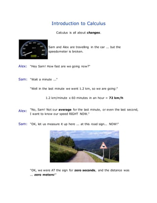
  • 1. Introduction to Calculus Calculus is all about changes. Sam and Alex are travelling in the car ... but the speedometer is broken. Alex: "Hey Sam! How fast are we going now?" Sam: "Wait a minute ..." "Well in the last minute we went 1.2 km, so we are going:" 1.2 km/minute x 60 minutes in an hour = 72 km/h Alex: "No, Sam! Not our average for the last minute, or even the last second, I want to know our speed RIGHT NOW." Sam: "OK, let us measure it up here ... at this road sign... NOW!" "OK, we were AT the sign for zero seconds, and the distance was ... zero meters!"
  • 2. The speed is 0m / 0s = 0/0 = I Don't Know! "I can't calculate it Sam! I need to know some distance over some time, and you are saying the time should be zero? Can't be done." That is pretty amazing ... you'd think it is easy to work out the speed of a car at any point in time, but it isn't. Even the speedometer of a car (when it works!) just shows us an average of how fast we were going for the last very short amount of time. How About Getting Real Close But our story is not finished yet! Sam and Alex get out of the car, because they have arrived on location. Sam is about to do a stunt: Sam will do a jump off a 20 m building. Alex, as photographer, asks: "How fast will you be falling after 1 second?" Sam uses this simplified formula to find the distance fallen: d = 5t2  d = distance fallen, in meters  t = time from jump, in seconds
  • 3. Example: at 1 second Sam has fallen d = 5t2 = 5 × 12 = 5 m But how fast is that? Speed is distance over time: Speed = distance time So at 1 second: Speed = 5 m = 5 m/s 1 second "BUT", says Alex, "again that is an average speed, since you started the jump, ... I want to know the speed at exactly 1 second, so I can set up the camera properly." Well ... at exactly 1 second the speed is: Speed = 5 − 5 m = 0 m = ???? 1 − 1 s 0 s So again Sam has a problem. Think about it ... how do we figure out a speed at an exact instant in time? What is the distance? What is the time difference? They are both zero, giving us nothing to calculate with! But Sam has an idea ... invent a time so short it won't matter. Sam won't even give it a value, and will just call it "Δt" (called "delta t").
  • 4. So Sam works out the difference in distance between t and t+Δt At 1 second Sam has fallen d = 5t2 = 5 × (1)2 = 5 m At (1+Δt) seconds Sam has fallen d = 5t2 = 5 × (1+Δt)2 m We can expand (1+Δt)2 : (1+Δt)2 = (1+Δt)(1+Δt) = 1 + 2Δt + (Δt)2 And we get: d = 5 × (1+2Δt+(Δt)2 ) m = 5 + 10Δt + 5(Δt)2 m So between 1 second and (1+Δt) seconds the distance fallen is: Change in d = (5 + 10Δt + 5(Δt)2 ) − 5 m = 10Δt + 5(Δt)2 m Now divide that distance by time to get the speed:
  • 5. Speed= 10Δt +5(Δt)2 mΔt s = 10 + 5Δt m/s So the speed is 10 + 5Δt m/s, and Sam thinks about that Δt value ... he wants Δt to be so small it won't matter ... so he imagines it shrinking towards zero and he gets: Speed = 10 m/s Wow! Sam got an answer! Sam: "I will be falling at exactly 10 m/s" Alex: "I thought you said you couldn't calculate it?" Sam: "That was before I used Calculus!" Yes, indeed, that was Calculus. The word Calculus comes from Latin meaning "small stone". Because it is like understanding something by looking at small pieces. Differential Calculus cuts something into small pieces to find how it changes.
  • 6. Integral Calculus joins (integrates) the small pieces together to find how much there is. And Differential Calculus and Integral Calculus are like inverses of each other, just like multiplication and division are inverses. Sam used Differential calculus to cut time and distance into such small pieces that a pure answer came out. So ... was Sam's result just luck? Does it work for other things? Let's try doing this for the function y = x3 This is going to be very similar to the previous example, but it will be just a slope on a graph, no one has to jump for this one! Example: What is the slope of the function y = x3 at x=1 ? At x = 1, y = 13 = 1 At x = (1+Δx), y = (1+Δx)3 We can expand (1+Δx)3 to 1 + 3Δx + 3(Δx)2 + (Δx)3 , and we get: y = 1 + 3Δx + 3(Δx)2 + (Δx)3 And the difference between the y values from x = 1 to x = 1+Δx is: Change in y = 1 + 3Δx + 3(Δx)2 + (Δx)3 − 1 = 3Δx + 3(Δx)2 + (Δx)3
  • 7. Now we can calculate slope: Slope = 3Δx + 3(Δx)2 + (Δx)3 Δx = 3 + 3Δx + (Δx)2 Once again, as Δx shrinks towards zero we are left with: Slope = 3 And here we see the graph of y = x3 The slope is continually changing, but at the point (1,1) we can draw a line tangent to the curve and find the slope there really is 3. (Count the squares if you want!) Question for you: what is the slope at the point (2,8)? Try It Yourself! Go to the Slope of a Function page, put in the formula "x^3", then try to find the slope at the point (1,1). Zoom in closer and closer and see what value the slope is heading towards.
  • 8. Conclusion Calculus is about changes. Differential calculus cuts something into small pieces to find how it changes.  Learn more at Introduction to Derivatives Integral calculus joins (integrates) the small pieces together to find how much there is.  Learn more at Introduction to Integration Introduction to Derivatives It is all about slope! Slope = Change in YChange in X We can find an average slope between two points.
  • 9. But how do we find the slope at a point? There is nothing to measure! But with derivatives we use a small difference ... ... then have it shrink towards zero. Let us Find a Derivative! We will use the slope formula: Slope = Change in YChange in X = ΔyΔx to find the derivative of a function y = f(x) x changes from x to x+Δx y changes from f(x) to f(x+Δx) Follow these steps:
  • 10. • Fill in this slope formula: ΔyΔx = f(x+Δx) − f(x)Δx • Simplify it as best we can, • Then make Δx shrink towards zero. Here we go: Example: the function f(x) = x2 We know f(x) = x2, and can calculate f(x+Δx) : Start with: f(x+Δx) = (x+Δx)2 Expand (x + Δx)2 : f(x+Δx) = x2 + 2x Δx + (Δx)2 The slope formula is: f(x+Δx) − f(x) Δx Put in f(x+Δx) and f(x): x2 + 2x Δx + (Δx)2 − x2 Δx Simplify (x2 and −x2 cancel): = 2x Δx + (Δx)2 Δx Simplify more (divide through by Δx): = 2x + Δx And then as Δx heads towards 0 we get: = 2x
  • 11. Result: the derivative of x2 is 2x We write dx instead of "Δx heads towards 0", so "the derivative of" is commonly written x2 = 2x "The derivative of x2 equals 2x" or simply "d dx of x2 equals 2x" What does x2 = 2x mean? It means that, for the function x2 , the slope or "rate of change" at any point is 2x. So when x=2 the slope is 2x = 4, as shown here: Or when x=5 the slope is 2x = 10, and so on. Note: sometimes f’(x) is also used for "the derivative of": f’(x) = 2x "The derivative of f(x) equals 2x"
  • 12. Let's try another example. Example: What is x3 ? We know f(x) = x3 , and can calculate f(x+Δx) : Start with: f(x+Δx) = (x+Δx)3 Expand (x + Δx)3 : f(x+Δx) = x3 + 3x2 Δx + 3x (Δx)2 + (Δx)3 The slope formula: f(x+Δx) − f(x) Δx Put in f(x+Δx) and f(x): x3 + 3x2 Δx + 3x (Δx)2 + (Δx)3 − x3 Δx Simplify (x3 and −x3 cancel): = 3x2 Δx + 3x (Δx)2 + (Δx)3 Δx Simplify more (divide through by Δx): = 3x2 + 3x Δx + (Δx)2 And then as Δx heads towards 0 we get: x3 = 3x2 Have a play with it using the Derivative Plotter. Derivatives of Other Functions We can use the same method to work out derivatives of other functions (like sine, cosine, logarithms, etc). But in practice the usual way to find derivatives is to use: Derivative Rules
  • 13. Example: what is the derivative of sin(x) ? On Derivative Rules it is listed as being cos(x) Done. Using the rules can be tricky! Example: what is the derivative of cos(x)sin(x) ? You can't just find the derivative of cos(x) and multiply it by the derivative of sin(x) ... you must use the "Product Rule" as explained on the Derivative Rules page. It actually works out to be cos2 (x) - sin2 (x) So that is your next step: learn how to use the rules. Notation "Shrink towards zero" is actually written as a limit like this: "The derivative of f equals the limit as Δx goes to zero of f(x+Δx) - f(x) over Δx" Or sometimes the derivative is written like this (explained on Derivatives as dy/dx):
  • 14. The process of finding a derivative is called "differentiation". You do differentiation ... to get a derivative. Rules of calculus - functions of one variable Derivatives: definitions, notation, and rules A derivative is a function which measures the slope. It depends upon x in some way, and is found by differentiating a function of the form y = f (x). When x is substituted into the derivative, the result is the slope of the original function y = f (x). There are many different ways to indicate the operation of differentiation, also known as finding or taking the derivative. The choice of notation depends on the type of function being evaluated and upon personal preference. Suppose you have a general function: y = f(x). All of the following notations can be read as "the derivative of y with respect to x" or less formally, "the derivative of the function." f'(x) f' y' df/dx dy/dx d/dx [f(x)]. [HINT: don't read the last three terms as fractions, read them as an operation. For example, read: " dx/dy = 3x" As: "the function that gives the slope is equal to 3x" Let's try some examples. Suppose we have the function : y = 4x3 + x2 + 3. After applying the rules of differentiation, we end up with the following result:
  • 15. dy/dx = 12x2 + 2x. How do we interpret this? First, decide what part of the original function (y = 4x3 + x2 + 3) you are interested in. For example, suppose you would like to know the slope of y when the variable x takes on a value of 2. Substitute x = 2 into the function of the slope and solve: dy/dx = 12 ( 2 )2 + 2 ( 2 ) = 48 + 4 = 52. Therefore, we have found that when x = 2, the function y has a slope of + 52. Now for the practical part. How do we actually determine the function of the slope? Almost all functions you will see in economics can be differentiated using a fairly short list of rules or formulas, which will be presented in the next several sections. How to apply the rules of differentiation Once you understand that differentiation is the process of finding the function of the slope, the actual application of the rules is straightforward. First, some overall strategy. The rules are applied to each term within a function separately. Then the results from the differentiation of each term are added together, being careful to preserve signs. [For example, the sum of 3x and negative 2x2 is 3x minus 2x2.]. Don't forget that a term such as "x" has a coefficient of positive one. Coefficients and signs must be correctly carried through all operations, especially in differentiation. The rules of differentiation are cumulative, in the sense that the more parts a function has, the more rules that have to be applied. Let's start here with some specific examples, and then the general rules will be presented in table form. Take the simple function: y = C, and let C be a constant, such as 15. The derivative of any constant term is 0, according to our first rule. This makes sense since slope is defined as the change in the y variable for a given change in the x variable. Suppose x goes from 10 to 11; y is still equal to 15 in this function, and does not change, therefore the slope is 0. Note that this function graphs as a horizontal line. Now, add another term to form the linear function y = 2x + 15. The next rule states that when the x is to the power of one, the slope is the coefficient on that x. This continues to make sense, since a change in x is multiplied by 2 to determine the
  • 16. resulting change in y. We add this to the derivative of the constant, which is 0 by our previous rule, and the slope of the total function is 2. Now, suppose that the variable is carried to some higher power. We can then form a typical nonlinear function such as y = 5x3 + 10. The power rule combined with the coefficient rule is used as follows: pull out the coefficient, multiply it by the power of x, then multiply that term by x, carried to the power of n - 1. Therefore, the derivative of 5x3 is equal to (5)(3)(x)(3 - 1); simplify to get 15x2. Add to the derivative of the constant which is 0, and the total derivative is 15x2. Note that we don't yet know the slope, but rather the formula for the slope. For a given x, such as x = 1, we can calculate the slope as 15. In plainer terms, when x is equal to 1, the function ( y = 5x3 + 10) has a slope of 15. These rules cover all polynomials, and now we add a few rules to deal with other types of nonlinear functions. It is not as obvious why the application of the rest of the rules still results in finding a function for the slope, and in a regular calculus class you would prove this to yourself repeatedly. Here, we want to focus on the economic application of calculus, so we'll take Newton's word for it that the rules work, memorize a few, and get on with the economics! The most important step for the remainder of the rules is to properly identify the form, or how the terms are combined, and then the application of the rule is straightforward. For functions that are sums or differences of terms, we can formalize the strategy above as follows: If y = f(x) + g(x), then dy/dx = f'(x) + g'(x). Here's a chance to practice reading the symbols. Read this rule as: if y is equal to the sum of two terms or functions, both of which depend upon x, then the function of the slope is equal to the sum of the derivatives of the two terms. If the total function is f minus g, then the derivative is the derivative of the f term minus the derivative of the g term. The product rule is applied to functions that are the product of two terms, which both depend on x, for example, y = (x - 3)(2x2 - 1). The most straightforward approach would be to multiply out the two terms, then take the derivative of the resulting polynomial according to the above rules. Or you have the option of applying the following rule. Given y = f(x) g(x); dy/dx = f'g + g'f. Read this as follows: the derivative of y with respect to x is the derivative of the f term multiplied by the g term, plus the derivative of the g term multiplied by the f term. To apply it to the above problem, note that f(x)
  • 17. = (x - 3) and g(x) = (2x2 - 1); f'(x) = 1 and g'(x) = 4x. Then dy/dx = (1)(2x2 - 1) + (4x)(x - 3). Simplify, and dy/dx = 2x2 - 1 + 4x2 - 12x, or 6x2 - 12x - 1. The quotient rule is similarly applied to functions where the f and g terms are a quotient. Suppose you have the function y = (x + 3)/ (- x2). Then follow this rule: Given y = f(x)/g(x), dy/dx = (f'g - g'f) / g2. Again, identify f= (x + 3) and g = -x2 ; f'(x) = 1 and g'(x) = - 2; and g2 = x4. Then substitute in: dy/dx = [(1)(- x2) - (- 2)(x + 3)] / x4 . Simplify to dy/dx = (-x2 + 2x + 6)/ x4 . Now, let's combine rules by type of function and their corresponding graphs. Type of function Form of function Graph Rule Interpretation y = constant y = C Horizontal line dy/dx = 0 Slope = 0; y = linear function y = ax + b Straight line dy/dx = a Slope = coefficient on x y = polynomial of order 2 or higher y = axn + b Nonlinear, one or more turning points dy/dx = anxn-1 Derivative is a function, actual slope depends upon location (ie value of x) y = sums or differences of 2 functions y = f(x) + g(x) Nonlinear dy/dx = f'(x) + g'(x). Take derivative of each term separately, then combine. y = product of two functions, y = [ f(x) g(x) ] Typically nonlinear dy/dx = f'g + g'f. Start by identifying f, g, f', g' y = quotient or ratio of two functions y = f ( x) / g ( x) Typically nonlinear dy/dx = (f'g - g'f) / g2. Start by identifying f, g, f', g', and g2 Not-so-basic rules of differentiation There are two more rules that you are likely to encounter in your economics studies. The hardest part of these rules is identifying to which parts of the functions the rules apply. Actually applying the rule is a simple matter of substituting in and multiplying through. Notice that the two rules of this section build upon the rules from the
  • 18. previous section, and provide you with ways to deal with increasingly complicated functions, while still using the same techniques. The power function rule: In the previous rules, we dealt with powers attached to a single variable, such as x2 , or x5. Suppose, however, that your equation carries more than just the single variable x to a power. For example, y = (2x + 3)4 In this case, the entire term (2x + 3) is being raised to the fourth power. To deal with cases like this, first identify and rename the inner term in the parenthesis: 2x + 3 = g(x). Then the problem becomes Now, note that your goal is still to take the derivative of y with respect to x. However, x is being operated on by two functions; first by g (multiplies x by 2 and adds to 3), and then that result is carried to the power of four. Therefore, when we take the derivatives, we have to account for both operations on x. First, use the power rule from the table above to get: . Note that the rule was applied to g(x) as a whole. Then take the derivative of g(x) = 2x + 3, using the appropriate rule from the table: . Note the change in notation. "g" is used because we were finding the change in g, with respect to a change in x. Now, both parts are multiplied to get the final result: Recall that derivatives are defined as being a function of x. Replace the g(x) in the above term with (2x + 3) in order to satisfy that requirement. Then simplify by combining the coefficients 4 and 2, and changing the power (4-1) to 3:
  • 19. Now, we can set up the general rule. When a function takes the following form: Then the rule for taking the derivative is: The chain rule: The second rule in this section is actually just a generalization of the above power rule. It is used when x is operated on more than once, but it isn't limited only to cases involving powers. Since you already understand the above problem, let's redo it using the chain rule, so you can focus on the technique. Given the same problem: rename the parts of the problem as follows: and Then the entire problem can be expressed as: This type of function is also known as a composite function. The derivative of a composite function is equal to the derivative of y with respect to u, times the derivative of u with respect to x:
  • 20. specifically in our problem: Recall that a derivative is defined as a function of x, not u. Substitute in 2x + 3 for u: and the problem is complete. The formal chain rule is as follows. When a function takes the following form: Then the derivative of y with respect to x is defined as: Updated table of derivatives Let's add these two rules to our table of derivatives from the previous section: Type of function Form of function Graph Rule Interpretation y = constant y = C Horizontal line dy/dx = 0 Slope = 0; y = linear function y = ax + b Straight line dy/dx = a Slope = coefficient on x y = polynomial of order 2 or higher y = axn + b Nonlinear, one or more turning points dy/dx = anxn-1 Derivative is a function, actual slope depends upon location (i.e. value of x) y = sums or differences of 2 functions y = f(x) + g(x) Nonlinear dy/dx = f'(x) + g'(x). Take derivative of each term separately, then
  • 21. combine. y = product of two functions y = [ f(x) g(x) ] Typically nonlinear dy/dx = f'g + g'f. Start by identifying f, g, f', g' y = quotient or ratio of two functions y = f ( x) / g ( x) Typically nonlinear dy/dx = (f'g - g'f) / g2. Start by identifying f, g, f', g', and g2 y=generalized power function Nonlinear Identify g(x) y=composite function/chain rule Nonlinear y is a function of u, and u is a function of x. Special cases There are two special cases of derivative rules that apply to functions that are used frequently in economic analysis. You may want to review the sections on natural logarithmic functions and graphs and exponential functions and graphs before starting this section. Natural logarithmic functions When a function takes the logarithmic form: Then the derivative of the function follows the rule: If the function y is a natural log of a function of y, then you use the log rule and the chain rule. For example, If the function is:
  • 22. Then we apply the chain rule, first by identifying the parts: Now, take the derivative of each part: And finally, multiply according to the rule. Now, replace the u with 5x2, and simplify Note that the generalized natural log rule is a special case of the chain rule: Then the derivative of y with respect to x is defined as: Exponential functions Taking the derivative of an exponential function is also a special case of the chain rule. First, let's start with a simple exponent and its derivative. When a function takes the logarithmic form: Then the derivative of the function follows the rule:
  • 23. . No, it's not a misprint! The derivative of ex is ex . If the power of e is a function of x, not just the variable x, then use the chain rule: Then the derivative of y with respect to x is defined as: For example, suppose you are taking the derivative of the following function: Define the parts y and u, and take their respective derivatives: Then the derivative of y with respect to x is: Updated table of derivatives Now we can add these two special cases to our table: Type of function Form of function Graph Rule Interpretatio n y = constant y = C Horizontal line dy/dx = 0 Slope = 0; y = linear function y = ax + b Straight line dy/dx = a Slope = coefficient on
  • 24. x y = polynomial of order 2 or higher y = axn + b Nonlinear, one or more turning points dy/dx = anxn-1 Derivative is a function, actual slope depends upon location (i.e. value of x) y = sums or differences of 2 functions y = f(x) + g(x) Nonlinear dy/dx = f'(x) + g'(x). Take derivative of each term separately, then combine. y = product of two functions, y = [ f(x) g(x) ] Typically nonlinear dy/dx = f'g + g'f. Start by identifying f, g, f', g' y = quotient or ratio of two functions y = f ( x) / g ( x) Typically nonlinear dy/dx = (f'g - g'f) / g2. Start by identifying f, g, f', g', and g2 y=generalized power function Nonlinear identify g(x) y=composite function/ chain rule Nonlinear y is a function of u, and u is a function of x. y=natural log function Natural log Special case of chain rule y=exponentia l function Exponentia l Special case of chain rule Higher order derivatives Just as a first derivative gives the slope or rate of change of a function, a higher order derivative gives the rate of change of the previous derivative. We'll tak more about
  • 25. how this fits into economic analysis in a future section, [link: economic interpretation of higher order derivatives] but for now, we'll just define the technique and then describe the behavior with a few simple examples. To find a higher order derivative, simply reapply the rules of differentiation to the previous derivative. For example, suppose you have the following function: According to our rules, we can find the formula for the slope by taking the first derivative: Take the second derivative by applying the rules again, this time to y', NOT y: If we need a third derivative, we differentiate the second derivative, and so on for each successive derivative. Note that the notation for second derivative is created by adding a second prime. Other notations are also based on the corresponding first derivative form. Here are some examples of the most common notations for derivatives and higher order derivatives. Function First derivative Second derivative Third derivative Now for some examples of what a higher order derivative actually is. Let's start with a nonlinear function and take a first and second derivative. Recall from previous sections that this equation will graph as a parabola that opens downward [link: graphing binomial functions].
  • 26. Function First derivative Second derivative In order to understand the meaning of derivatives, let's pick a couple of values of x, and calculate the value of the derivatives at those points. Value of x Value of function at x first derivative at x second derivative at x x=0 x=1 x=2 So, how do we interpret this information? When x equals 0, we know that the slope of the function, or rate of change in y for a given change in x (from the first derivative) is 6. Similarly, the second derivative tells us that the rate of change of the first derivative for a given change in x is -2. In other words, when x changes, we expect the slope to change by -2, or to decrease by 2. We can check this by changing
  • 27. x from 0 to 1, and noting that the slope did change from 6 to 4, therefore decreasing by 2. To sum up, the first derivative gives us the slope, and the second derivative gives the change in the slope. In economics, the first two derivatives will be the most useful, so we'll stop there for now. [Index] Higher Order Derivatives Because the derivative of a function y = f( x) is itself a function y′ = f′( x), you can take the derivative of f′( x), which is generally referred to as thesecond derivative of f(x) and written f“( x) or f 2( x). This differentiation process can be continued to find the third, fourth, and successive derivatives of f( x), which are called higher order derivatives of f( x). Because the “prime” notation for derivatives would eventually become somewhat messy, it is preferable to use the numerical notation f( n )( x) =y( n ) to denote the nth derivative of f( x). Example 1: Find the first, second, and third derivatives of f( x) = 5 x 4 − 3x 3 + 7x 2 − 9x + 2.
  • 28. Example 2: Find the first, second, and third derivatives of y = sin 2 x. Example 3: Find f (3) (4) if . Higher Order Derivatives Let’s start this section with the following function.
  • 29. By this point we should be able to differentiate this function without any problems. Doing this we get, Now, this is a function and so it can be differentiated. Here is the notation that we’ll use for that, as well as the derivative. This is called the second derivative and is now called the first derivative. Again, this is a function so we can differentiate it again. This will be called the third derivative. Here is that derivative as well as the notation for the third derivative. Continuing, we can differentiate again. This is called, oddly enough, the fourth derivative. We’re also going to be changing notation at this point. We can keep adding on primes, but that will get cumbersome after awhile. This process can continue but notice that we will get zero for all derivatives after this point. This set of derivatives leads us to the following fact about the differentiation of polynomials. Fact If p(x) is a polynomial of degree n (i.e. the largest exponent in the polynomial) then,
  • 30. We will need to be careful with the “non-prime” notation for derivatives. Consider each of the following. The presence of parenthesis in the exponent denotes differentiation while the absence of parenthesis denotes exponentiation. Collectively the second, third, fourth, etc. derivatives are called higher order derivatives. Let’s take a look at some examples of higher order derivatives. Example 1 Find the first four derivatives for each of the following. (a) [Solution] (b) [Solution] (c) [Solution] Solution (a) There really isn’t a lot to do here other than do the derivatives.
  • 31. Notice that differentiating an exponential function is very simple. It doesn’t change with each differentiation. [Return to Problems] (b) Again, let’s just do some derivatives. Note that cosine (and sine) will repeat every four derivatives. The other four trig functions will not exhibit this behavior. You might want to take a few derivatives to convince yourself of this. [Return to Problems] (c) In the previous two examples we saw some patterns in the differentiation of exponential functions, cosines and sines. We need to be careful however since they only work if there is just a t or an x in the argument. This is the point of this example. In this example we will need to use the chain rule on each derivative.
  • 32. So, we can see with slightly more complicated arguments the patterns that we saw for exponential functions, sines and cosines no longer completely hold. [Return to Problems] Let’s do a couple more examples to make a couple of points. Example 2 Find the second derivative for each of the following functions. (a) [Solution] (b) [Solution] (c) [Solution] Solution (a) Here’s the first derivative. Notice that the second derivative will now require the product rule.
  • 33. Notice that each successive derivative will require a product and/or chain rule and that as noted above this will not end up returning back to just a secant after four (or another other number for that matter) derivatives as sine and cosine will. [Return to Problems] (b) Again, let’s start with the first derivative. As with the first example we will need the product rule for the second derivative. [Return to Problems] (c) Same thing here. The second derivative this time will require the quotient rule.
  • 34. [Return to Problems] As we saw in this last set of examples we will often need to use the product or quotient rule for the higher order derivatives, even when the first derivative didn’t require these rules. Let’s work one more example that will illustrate how to use implicit differentiation to find higher order derivatives. Example 3 Find for Solution Okay, we know that in order to get the second derivative we need the first derivative and in order to get that we’ll need to do implicit differentiation. Here is the work for that. Now, this is the first derivative. We get the second derivative by differentiating this, which will require implicit differentiation again.
  • 35. This is fine as far as it goes. However, we would like there to be no derivatives in the answer. We don’t, generally, mind having x’s and/or y’s in the answer when doing implicit differentiation, but we really don’t like derivatives in the answer. We can get rid of the derivative however by acknowledging that we know what the first derivative is and substituting this into the second derivative equation. Doing this gives,
  • 36. Now that we’ve found some higher order derivatives we should probably talk about an interpretation of the second derivative. If the position of an object is given by s(t) we know that the velocity is the first derivative of the position. The acceleration of the object is the first derivative of the velocity, but since this is the first derivative of the position function we can also think of the acceleration as the second derivative of the position function. Alternate Notation There is some alternate notation for higher order derivatives as well. Recall that there was a fractional notation for the first derivative.
  • 37. We can extend this to higher order derivatives. Basic Concepts of Optimization The concept of optimization is basic to much of what we do in our daily lives: a desire to do better or be the best in one field or another. In engineering we wish to produce the best possible result with the available resources. In a highly competitive modern world it is no longer sufficient to design a system whose performance of the required task is just satisfactory. It is essential to design the best system. Thus in “designing” new products in any field: aerospace, automotive, chemical, electrical, biomedical, agricultural, etc, we must use design tools which provide the desired results in a timely and economical fashion. Numerical optimization is one of the tools at our disposal. Optimization is a very general automated design technique. In studying this technique it is important to distinguish between analysis and design. Analysis is the process of determining the response of the specified system to the certain combination of input parameters. For example, calculatin stresses in the structure as a result of certain loads. Design on the other hand, means the process of defining a system. For example, designing a structure would mean selecting specific dimensions and location of the structural members that will allow the structure to withstand the specified load. Much of the design task in engineering is quantifiable, and so we are able to use computers to analyze alternative designs rapidly. The purpose of numerical optimization is to aid us in rationally searching among alternative designs for the best design to meet our needs. The alternative designs of the same system differ from each other because some parameters of the system are not the same. The parameters that could be changed in the system while searching for the best design are called design variables. Although we may not always think of it this way, design process may be defined as the process of finding the minimum or maximum of some characteristic, which may be called the objective function. For the design to be acceptable it must also satisfy certain requirements. These requirements are called design constraints. Optimization automatically changes the design
  • 38. variables to help us find the minimum or maximum of the objective function, while satisfying all the required design constraints. Figure 1. Locate the top of the hill while blindfolded. Consider example in Figure 1. One boy bets that he can locate the top of the hill while blindfolded. The other boy agrees but asks the first boy to also stay inside the fences. Translating this situation into optimization problem formulation, we see that the objective is to find the highest point on the hill. Therefore, objective function is the height achieved by the first boy with respect to his original position. The design variables are longitude and latitude – the coordinates, defining position of the boy. The constraints are that the boy has to stay inside the fences. Note here, that in general, the boy may start the search from outside the fences. It is possible to define this physical problem mathematically, thus converting it to the engineering problem as shown in Figure 2: Figure 2. Engineering problem formulation for the physical problem Optimization is a very simple extension of the engineering problem:
  • 39. Maximize: (objective) Subject to: (constraints) (design variables) Recall, that optimization automatically changes the design variables to helps us find the minimum or maximum of the objective function, while satisfying all the required constraints. The optimization process is illustrated in Figure 3. It may be broken down into the following steps: • Find a search direction that will improve the objective while staying inside the fences; • Search in this direction until no more improvement can be made by going in this direction; • Repeat the process, until no search direction can be found that improves the objective. Figure 3. Optimization process. The optimization problem formulation and the optimization process presented above are very general and can be applied to any design problem in any field. For example, if we wish to design the internal combustion engine, the objective may be to maximize the combustion efficiency. The engine may be required to provide a specific power output with an upper limit on the amount of harmful pollutants emitted into the atmosphere. These parameters will serve as constraints for optimization. The design variables that are allowed to be changed during optimization may be the compression ratio, air-fuel mixture ratio, bore and stroke, etc. Optimization is not limited to engineering only. It is possible to optimize the financial portfolio, optimize the revenue and expenditures of a company, optimize the route of a delivery truck, optimize the chemical processing, optimize protein models, etc. It is not debatable that optimization is useful. It has been successfully working for many years. However, at the same time it is by no means a replacement for a designer. It is also not a “push-button” tool that instantly produces the best design without human intervention. It is a process that reduces the design time, improves the design quality, and free engineers and designers for creative work by taking over tedious operations.
  • 40. Optimization is the most powerful design improvement tool that is available today!