Descargar como PDF, PPTX


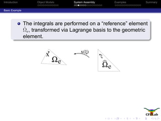
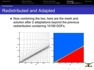
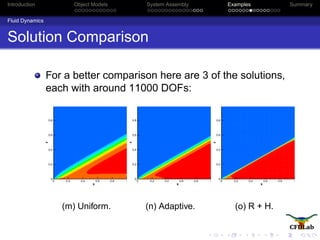
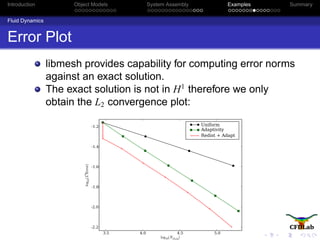
![Introduction Object Models System Assembly Examples Summary
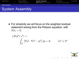
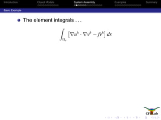
Basic Example
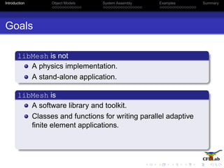
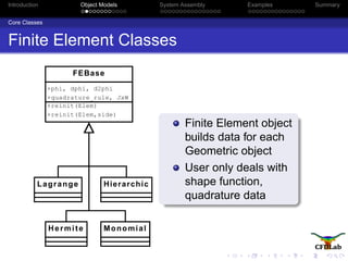
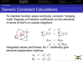
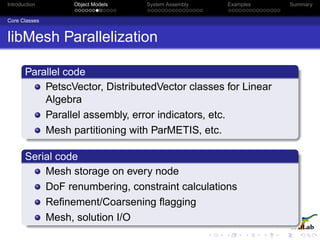
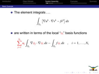
At the qth quadrature point, LibMesh can provide
variables including:
Code Math Description
JxW[q] |J(ξq)|wq Jacobian times weight
phi[i][q] φi(ξq) value of ith
shape fn.
dphi[i][q] φi(ξq) value of ith
shape fn. gradient
d2phi[i][q] φi(ξq) value of ith
shape fn. Hessian
xyz[q] x(ξq) location of ξq in physical space
normals[q] n(x(ξq)) normal vector at x on a side](https://image.slidesharecdn.com/sandialibmesh-130818143356-phpapp01/85/Finite-Elements-libmesh-52-320.jpg)
![Introduction Object Models System Assembly Examples Summary
Basic Example
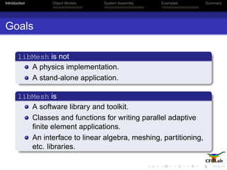
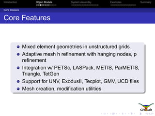
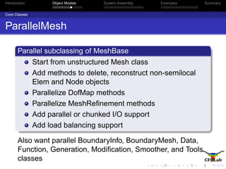
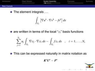
The LibMesh representation of the matrix and rhs
assembly is similar to the mathematical statements.
for (q=0; q<Nq; ++q)
for (i=0; i<Ns; ++i) {
Fe(i) += JxW[q]*f(xyz[q])*phi[i][q];
for (j=0; j<Ns; ++j)
Ke(i,j) += JxW[q]*(dphi[j][q]*dphi[i][q]);
}](https://image.slidesharecdn.com/sandialibmesh-130818143356-phpapp01/85/Finite-Elements-libmesh-53-320.jpg)
![Introduction Object Models System Assembly Examples Summary
Basic Example
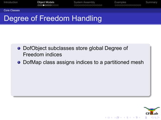
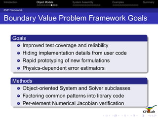
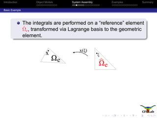
The LibMesh representation of the matrix and rhs
assembly is similar to the mathematical statements.
for (q=0; q<Nq; ++q)
for (i=0; i<Ns; ++i) {
Fe(i) += JxW[q]*f(xyz[q])*phi[i][q];
for (j=0; j<Ns; ++j)
Ke(i,j) += JxW[q]*(dphi[j][q]*dphi[i][q]);
}
Fe
i =
Nq
q=1
f(x(ξq))φi(ξq)|J(ξq)|wq](https://image.slidesharecdn.com/sandialibmesh-130818143356-phpapp01/85/Finite-Elements-libmesh-54-320.jpg)
![Introduction Object Models System Assembly Examples Summary
Basic Example
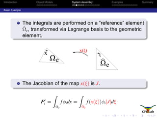
The LibMesh representation of the matrix and rhs
assembly is similar to the mathematical statements.
for (q=0; q<Nq; ++q)
for (i=0; i<Ns; ++i) {
Fe(i) += JxW[q]*f(xyz[q])*phi[i][q];
for (j=0; j<Ns; ++j)
Ke(i,j) += JxW[q]*(dphi[j][q]*dphi[i][q]);
}
Fe
i =
Nq
q=1
f(x(ξq))φi(ξq)|J(ξq)|wq](https://image.slidesharecdn.com/sandialibmesh-130818143356-phpapp01/85/Finite-Elements-libmesh-55-320.jpg)
![Introduction Object Models System Assembly Examples Summary
Basic Example
The LibMesh representation of the matrix and rhs
assembly is similar to the mathematical statements.
for (q=0; q<Nq; ++q)
for (i=0; i<Ns; ++i) {
Fe(i) += JxW[q]*f(xyz[q])*phi[i][q];
for (j=0; j<Ns; ++j)
Ke(i,j) += JxW[q]*(dphi[j][q]*dphi[i][q]);
}
Fe
i =
Nq
q=1
f(x(ξq))φi(ξq)|J(ξq)|wq](https://image.slidesharecdn.com/sandialibmesh-130818143356-phpapp01/85/Finite-Elements-libmesh-56-320.jpg)
![Introduction Object Models System Assembly Examples Summary
Basic Example
The LibMesh representation of the matrix and rhs
assembly is similar to the mathematical statements.
for (q=0; q<Nq; ++q)
for (i=0; i<Ns; ++i) {
Fe(i) += JxW[q]*f(xyz[q])*phi[i][q];
for (j=0; j<Ns; ++j)
Ke(i,j) += JxW[q]*(dphi[j][q]*dphi[i][q]);
}
Fe
i =
Nq
q=1
f(x(ξq))φi(ξq)|J(ξq)|wq](https://image.slidesharecdn.com/sandialibmesh-130818143356-phpapp01/85/Finite-Elements-libmesh-57-320.jpg)
![Introduction Object Models System Assembly Examples Summary
Basic Example
The LibMesh representation of the matrix and rhs
assembly is similar to the mathematical statements.
for (q=0; q<Nq; ++q)
for (i=0; i<Ns; ++i) {
Fe(i) += JxW[q]*f(xyz[q])*phi[i][q];
for (j=0; j<Ns; ++j)
Ke(i,j) += JxW[q]*(dphi[j][q]*dphi[i][q]);
}
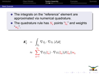
Ke
ij =
Nq
q=1
ˆξφj(ξq) · ˆξφi(ξq)|J(ξq)|wq](https://image.slidesharecdn.com/sandialibmesh-130818143356-phpapp01/85/Finite-Elements-libmesh-58-320.jpg)
![Introduction Object Models System Assembly Examples Summary
Basic Example
The LibMesh representation of the matrix and rhs
assembly is similar to the mathematical statements.
for (q=0; q<Nq; ++q)
for (i=0; i<Ns; ++i) {
Fe(i) += JxW[q]*f(xyz[q])*phi[i][q];
for (j=0; j<Ns; ++j)
Ke(i,j) += JxW[q]*(dphi[j][q]*dphi[i][q]);
}
Ke
ij =
Nq
q=1
ˆξφj(ξq) · ˆξφi(ξq)|J(ξq)|wq](https://image.slidesharecdn.com/sandialibmesh-130818143356-phpapp01/85/Finite-Elements-libmesh-59-320.jpg)
![Introduction Object Models System Assembly Examples Summary
Basic Example
The LibMesh representation of the matrix and rhs
assembly is similar to the mathematical statements.
for (q=0; q<Nq; ++q)
for (i=0; i<Ns; ++i) {
Fe(i) += JxW[q]*f(xyz[q])*phi[i][q];
for (j=0; j<Ns; ++j)
Ke(i,j) += JxW[q]*(dphi[j][q]*dphi[i][q]);
}
Ke
ij =
Nq
q=1
ˆξφj(ξq) · ˆξφi(ξq)|J(ξq)|wq](https://image.slidesharecdn.com/sandialibmesh-130818143356-phpapp01/85/Finite-Elements-libmesh-60-320.jpg)
![Introduction Object Models System Assembly Examples Summary
Basic Example
Convection-Diffusion Equation
The matrix assembly routine for the linear
convection-diffusion equation,
−k∆u + b · u = f
for (q=0; q<Nq; ++q)
for (i=0; i<Ns; ++i) {
Fe(i) += JxW[q]*f(xyz[q])*phi[i][q];
for (j=0; j<Ns; ++j)
Ke(i,j) += JxW[q]*(k*(dphi[j][q]*dphi[i][q])
+ (b*dphi[j][q])*phi[i][q]);
}](https://image.slidesharecdn.com/sandialibmesh-130818143356-phpapp01/85/Finite-Elements-libmesh-61-320.jpg)
![Introduction Object Models System Assembly Examples Summary
Basic Example
Convection-Diffusion Equation
The matrix assembly routine for the linear
convection-diffusion equation,
−k∆u + b · u = f
for (q=0; q<Nq; ++q)
for (i=0; i<Ns; ++i) {
Fe(i) += JxW[q]*f(xyz[q])*phi[i][q];
for (j=0; j<Ns; ++j)
Ke(i,j) += JxW[q]*(k*(dphi[j][q]*dphi[i][q])
+ (b*dphi[j][q])*phi[i][q]);
}](https://image.slidesharecdn.com/sandialibmesh-130818143356-phpapp01/85/Finite-Elements-libmesh-62-320.jpg)
![Introduction Object Models System Assembly Examples Summary
Basic Example
Convection-Diffusion Equation
The matrix assembly routine for the linear
convection-diffusion equation,
−k∆u + b · u = f
for (q=0; q<Nq; ++q)
for (i=0; i<Ns; ++i) {
Fe(i) += JxW[q]*f(xyz[q])*phi[i][q];
for (j=0; j<Ns; ++j)
Ke(i,j) += JxW[q]*(k*(dphi[j][q]*dphi[i][q])
+ (b*dphi[j][q])*phi[i][q]);
}](https://image.slidesharecdn.com/sandialibmesh-130818143356-phpapp01/85/Finite-Elements-libmesh-63-320.jpg)
![Introduction Object Models System Assembly Examples Summary
Coupled Variables
Stokes Flow
For multi-variable systems like Stokes flow,
p − ν∆u = f
· u = 0
∈ Ω ⊂ R2
The element stiffness matrix concept can extended to
include sub-matrices
Ke
u1u1
Ke
u1u2
Ke
u1p
Ke
u2u1
Ke
u2u2
Ke
u2p
Ke
pu1
Ke
pu2
Ke
pp
Ue
u1
Ue
u2
Ue
p
−
Fe
u1
Fe
u2
Fe
p
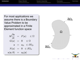
We have an array of submatrices: Ke[ ][ ]](https://image.slidesharecdn.com/sandialibmesh-130818143356-phpapp01/85/Finite-Elements-libmesh-64-320.jpg)
![Introduction Object Models System Assembly Examples Summary
Coupled Variables
Stokes Flow
For multi-variable systems like Stokes flow,
p − ν∆u = f
· u = 0
∈ Ω ⊂ R2
The element stiffness matrix concept can extended to
include sub-matrices
Ke
u1u1
Ke
u1u2
Ke
u1p
Ke
u2u1
Ke
u2u2
Ke
u2p
Ke
pu1
Ke
pu2
Ke
pp
Ue
u1
Ue
u2
Ue
p
−
Fe
u1
Fe
u2
Fe
p
We have an array of submatrices: Ke[1][1]](https://image.slidesharecdn.com/sandialibmesh-130818143356-phpapp01/85/Finite-Elements-libmesh-65-320.jpg)
![Introduction Object Models System Assembly Examples Summary
Coupled Variables
Stokes Flow
For multi-variable systems like Stokes flow,
p − ν∆u = f
· u = 0
∈ Ω ⊂ R2
The element stiffness matrix concept can extended to
include sub-matrices
Ke
u1u1
Ke
u1u2
Ke
u1p
Ke
u2u1
Ke
u2u2
Ke
u2p
Ke
pu1
Ke
pu2
Ke
pp
Ue
u1
Ue
u2
Ue
p
−
Fe
u1
Fe
u2
Fe
p
We have an array of submatrices: Ke[2][2]](https://image.slidesharecdn.com/sandialibmesh-130818143356-phpapp01/85/Finite-Elements-libmesh-66-320.jpg)
![Introduction Object Models System Assembly Examples Summary
Coupled Variables
Stokes Flow
For multi-variable systems like Stokes flow,
p − ν∆u = f
· u = 0
∈ Ω ⊂ R2
The element stiffness matrix concept can extended to
include sub-matrices
Ke
u1u1
Ke
u1u2
Ke
u1p
Ke
u2u1
Ke
u2u2
Ke
u2p
Ke
pu1
Ke
pu2
Ke
pp
Ue
u1
Ue
u2
Ue
p
−
Fe
u1
Fe
u2
Fe
p
We have an array of submatrices: Ke[3][2]](https://image.slidesharecdn.com/sandialibmesh-130818143356-phpapp01/85/Finite-Elements-libmesh-67-320.jpg)
![Introduction Object Models System Assembly Examples Summary
Coupled Variables
Stokes Flow
For multi-variable systems like Stokes flow,
p − ν∆u = f
· u = 0
∈ Ω ⊂ R2
The element stiffness matrix concept can extended to
include sub-matrices
Ke
u1u1
Ke
u1u2
Ke
u1p
Ke
u2u1
Ke
u2u2
Ke
u2p
Ke
pu1
Ke
pu2
Ke
pp
Ue
u1
Ue
u2
Ue
p
−
Fe
u1
Fe
u2
Fe
p
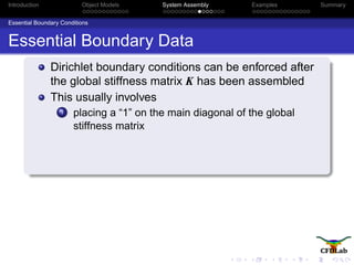
And an array of right-hand sides: Fe[].](https://image.slidesharecdn.com/sandialibmesh-130818143356-phpapp01/85/Finite-Elements-libmesh-68-320.jpg)
![Introduction Object Models System Assembly Examples Summary
Coupled Variables
Stokes Flow
For multi-variable systems like Stokes flow,
p − ν∆u = f
· u = 0
∈ Ω ⊂ R2
The element stiffness matrix concept can extended to
include sub-matrices
Ke
u1u1
Ke
u1u2
Ke
u1p
Ke
u2u1
Ke
u2u2
Ke
u2p
Ke
pu1
Ke
pu2
Ke
pp
Ue
u1
Ue
u2
Ue
p
−
Fe
u1
Fe
u2
Fe
p
And an array of right-hand sides: Fe[1].](https://image.slidesharecdn.com/sandialibmesh-130818143356-phpapp01/85/Finite-Elements-libmesh-69-320.jpg)
![Introduction Object Models System Assembly Examples Summary
Coupled Variables
Stokes Flow
For multi-variable systems like Stokes flow,
p − ν∆u = f
· u = 0
∈ Ω ⊂ R2
The element stiffness matrix concept can extended to
include sub-matrices
Ke
u1u1
Ke
u1u2
Ke
u1p
Ke
u2u1
Ke
u2u2
Ke
u2p
Ke
pu1
Ke
pu2
Ke
pp
Ue
u1
Ue
u2
Ue
p
−
Fe
u1
Fe
u2
Fe
p
And an array of right-hand sides: Fe[2].](https://image.slidesharecdn.com/sandialibmesh-130818143356-phpapp01/85/Finite-Elements-libmesh-70-320.jpg)
 += JxW[q]*f(xyz[q],d)*phi[i][q];
for (j=0; j<Ns; ++j)
Ke[d][d](i,j) +=
JxW[q]*nu*(dphi[j][q]*dphi[i][q]);
}](https://image.slidesharecdn.com/sandialibmesh-130818143356-phpapp01/85/Finite-Elements-libmesh-71-320.jpg)

![Introduction Object Models System Assembly Examples Summary
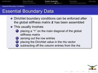
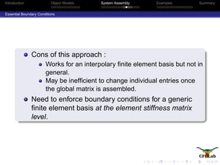
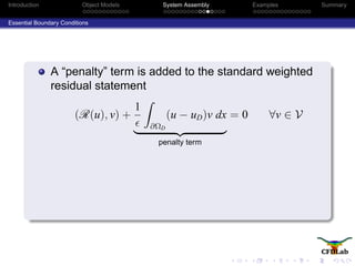
Essential Boundary Conditions
LibMesh provides:
A quadrature rule with Nqf points and JxW f[]
A finite element coincident with the boundary face
that has shape function values phi f[][]
for (qf=0; qf<Nqf; ++qf) {
for (i=0; i<Nf; ++i) {
Fe(i) += JxW_f[qf]*
penalty*uD(xyz[q])*phi_f[i][qf];
for (j=0; j<Nf; ++j)
Ke(i,j) += JxW_f[qf]*
penalty*phi_f[j][qf]*phi_f[i][qf];
}
}](https://image.slidesharecdn.com/sandialibmesh-130818143356-phpapp01/85/Finite-Elements-libmesh-84-320.jpg)
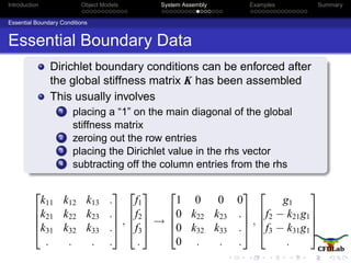
![Introduction Object Models System Assembly Examples Summary
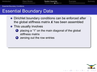
Essential Boundary Conditions
LibMesh provides:
A quadrature rule with Nqf points and JxW f[]
A finite element coincident with the boundary face
that has shape function values phi f[][]
for (qf=0; qf<Nqf; ++qf) {
for (i=0; i<Nf; ++i) {
Fe(i) += JxW_f[qf]*
penalty*uD(xyz[q])*phi_f[i][qf];
for (j=0; j<Nf; ++j)
Ke(i,j) += JxW_f[qf]*
penalty*phi_f[j][qf]*phi_f[i][qf];
}
}](https://image.slidesharecdn.com/sandialibmesh-130818143356-phpapp01/85/Finite-Elements-libmesh-85-320.jpg)
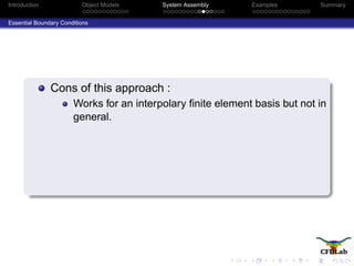
![Introduction Object Models System Assembly Examples Summary
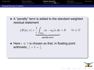
Essential Boundary Conditions
LibMesh provides:
A quadrature rule with Nqf points and JxW f[]
A finite element coincident with the boundary face
that has shape function values phi f[][]
for (qf=0; qf<Nqf; ++qf) {
for (i=0; i<Nf; ++i) {
Fe(i) += JxW_f[qf]*
penalty*uD(xyz[q])*phi_f[i][qf];
for (j=0; j<Nf; ++j)
Ke(i,j) += JxW_f[qf]*
penalty*phi_f[j][qf]*phi_f[i][qf];
}
}](https://image.slidesharecdn.com/sandialibmesh-130818143356-phpapp01/85/Finite-Elements-libmesh-86-320.jpg)

![Introduction Object Models System Assembly Examples Summary
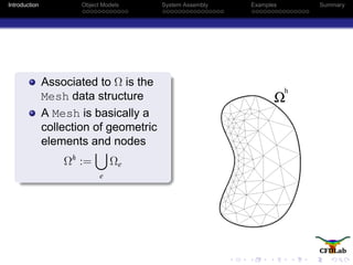
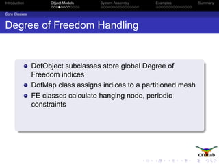
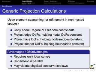
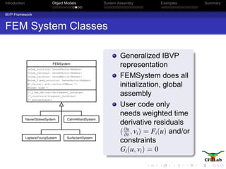
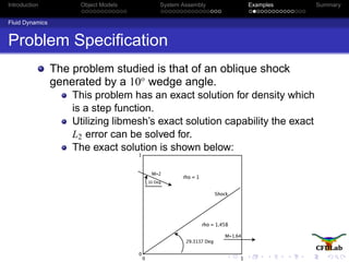
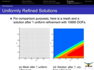
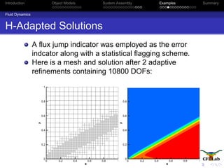
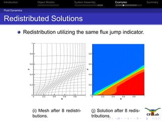
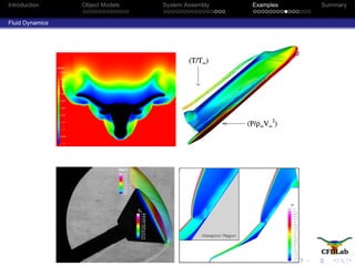
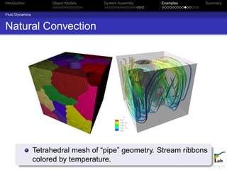
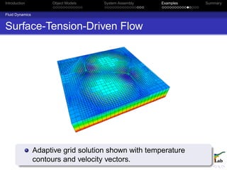
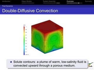
Fluid Dynamics
Instead of explicitly finding the Jacobian, we’ll use FEMSystem to finite difference the weak form.
element constraint()
for (unsigned int qp=0; qp != n_qpoints; qp++) {
Number u = interior_value(0, qp);
Gradient grad_u = interior_gradient(0, qp);
Number K = 1. / sqrt(1. + (grad_u * grad_u));
for (unsigned int i=0; i != n_u_dofs; i++) {
Fu(i) += JxW[qp] * ((_kappa * u * phi[i][qp]) +
(K * grad_u * dphi[i][qp]));
}
}
side constraint()
for (unsigned int qp=0; qp != n_qpoints; qp++) {
for (unsigned int i=0; i != n_u_dofs; i++) {
Fu(i) -= JxW[qp] * _gamma * phi[i][qp];
}
}
0
B
@
u
q
1 + | u|2
, ϕ
1
C
A
Ω
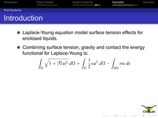
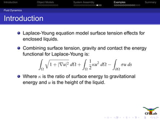
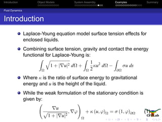
+ κ (u, ϕ)Ω − σ (1, ϕ)∂Ω = 0 ∀ϕ ∈ V](https://image.slidesharecdn.com/sandialibmesh-130818143356-phpapp01/85/Finite-Elements-libmesh-92-320.jpg)
![Introduction Object Models System Assembly Examples Summary
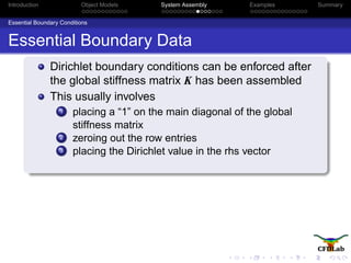
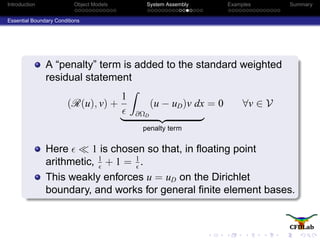
Fluid Dynamics
Instead of explicitly finding the Jacobian, we’ll use FEMSystem to finite difference the weak form.
element constraint()
for (unsigned int qp=0; qp != n_qpoints; qp++) {
Number u = interior_value(0, qp);
Gradient grad_u = interior_gradient(0, qp);
Number K = 1. / sqrt(1. + (grad_u * grad_u));
for (unsigned int i=0; i != n_u_dofs; i++) {
Fu(i) += JxW[qp] * ((_kappa * u * phi[i][qp]) +
(K * grad_u * dphi[i][qp]));
}
}
side constraint()
for (unsigned int qp=0; qp != n_qpoints; qp++) {
for (unsigned int i=0; i != n_u_dofs; i++) {
Fu(i) -= JxW[qp] * _gamma * phi[i][qp];
}
}
0
B
@
u
q
1 + | u|2
, ϕ
1
C
A
Ω
+ κ (u, ϕ)Ω − σ (1, ϕ)∂Ω = 0 ∀ϕ ∈ V](https://image.slidesharecdn.com/sandialibmesh-130818143356-phpapp01/85/Finite-Elements-libmesh-93-320.jpg)
![Introduction Object Models System Assembly Examples Summary
Fluid Dynamics
Instead of explicitly finding the Jacobian, we’ll use FEMSystem to finite difference the weak form.
element constraint()
for (unsigned int qp=0; qp != n_qpoints; qp++) {
Number u = interior_value(0, qp);
Gradient grad_u = interior_gradient(0, qp);
Number K = 1. / sqrt(1. + (grad_u * grad_u));
for (unsigned int i=0; i != n_u_dofs; i++) {
Fu(i) += JxW[qp] * ((_kappa * u * phi[i][qp]) +
(K * grad_u * dphi[i][qp]));
}
}
side constraint()
for (unsigned int qp=0; qp != n_qpoints; qp++) {
for (unsigned int i=0; i != n_u_dofs; i++) {
Fu(i) -= JxW[qp] * _gamma * phi[i][qp];
}
}
0
B
@
u
q
1 + | u|2
, ϕ
1
C
A
Ω
+ κ (u, ϕ)Ω − σ (1, ϕ)∂Ω = 0 ∀ϕ ∈ V](https://image.slidesharecdn.com/sandialibmesh-130818143356-phpapp01/85/Finite-Elements-libmesh-94-320.jpg)
![Introduction Object Models System Assembly Examples Summary
Fluid Dynamics
Instead of explicitly finding the Jacobian, we’ll use FEMSystem to finite difference the weak form.
element constraint()
for (unsigned int qp=0; qp != n_qpoints; qp++) {
Number u = interior_value(0, qp);
Gradient grad_u = interior_gradient(0, qp);
Number K = 1. / sqrt(1. + (grad_u * grad_u));
for (unsigned int i=0; i != n_u_dofs; i++) {
Fu(i) += JxW[qp] * ((_kappa * u * phi[i][qp]) +
(K * grad_u * dphi[i][qp]));
}
}
side constraint()
for (unsigned int qp=0; qp != n_qpoints; qp++) {
for (unsigned int i=0; i != n_u_dofs; i++) {
Fu(i) -= JxW[qp] * _gamma * phi[i][qp];
}
}
0
B
@
u
q
1 + | u|2
, ϕ
1
C
A
Ω
+ κ (u, ϕ)Ω − σ (1, ϕ)∂Ω = 0 ∀ϕ ∈ V](https://image.slidesharecdn.com/sandialibmesh-130818143356-phpapp01/85/Finite-Elements-libmesh-95-320.jpg)
![Introduction Object Models System Assembly Examples Summary
Fluid Dynamics
Instead of explicitly finding the Jacobian, we’ll use FEMSystem to finite difference the weak form.
element constraint()
for (unsigned int qp=0; qp != n_qpoints; qp++) {
Number u = interior_value(0, qp);
Gradient grad_u = interior_gradient(0, qp);
Number K = 1. / sqrt(1. + (grad_u * grad_u));
for (unsigned int i=0; i != n_u_dofs; i++) {
Fu(i) += JxW[qp] * ((_kappa * u * phi[i][qp]) +
(K * grad_u * dphi[i][qp]));
}
}
side constraint()
for (unsigned int qp=0; qp != n_qpoints; qp++) {
for (unsigned int i=0; i != n_u_dofs; i++) {
Fu(i) -= JxW[qp] * _gamma * phi[i][qp];
}
}
0
B
@
u
q
1 + | u|2
, ϕ
1
C
A
Ω
+ κ (u, ϕ)Ω − σ (1, ϕ)∂Ω = 0 ∀ϕ ∈ V](https://image.slidesharecdn.com/sandialibmesh-130818143356-phpapp01/85/Finite-Elements-libmesh-96-320.jpg)
![Introduction Object Models System Assembly Examples Summary
Fluid Dynamics
Instead of explicitly finding the Jacobian, we’ll use FEMSystem to finite difference the weak form.
element constraint()
for (unsigned int qp=0; qp != n_qpoints; qp++) {
Number u = interior_value(0, qp);
Gradient grad_u = interior_gradient(0, qp);
Number K = 1. / sqrt(1. + (grad_u * grad_u));
for (unsigned int i=0; i != n_u_dofs; i++) {
Fu(i) += JxW[qp] * ((_kappa * u * phi[i][qp]) +
(K * grad_u * dphi[i][qp]));
}
}
side constraint()
for (unsigned int qp=0; qp != n_qpoints; qp++) {
for (unsigned int i=0; i != n_u_dofs; i++) {
Fu(i) -= JxW[qp] * _gamma * phi[i][qp];
}
}
0
B
@
u
q
1 + | u|2
, ϕ
1
C
A
Ω
+ κ (u, ϕ)Ω − σ (1, ϕ)∂Ω = 0 ∀ϕ ∈ V](https://image.slidesharecdn.com/sandialibmesh-130818143356-phpapp01/85/Finite-Elements-libmesh-97-320.jpg)
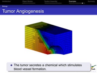
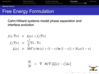
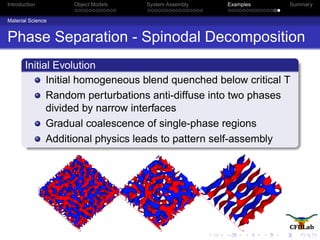
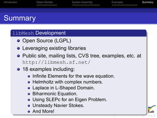

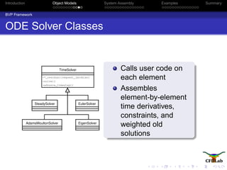
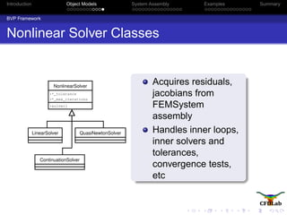
El documento presenta libMesh, una biblioteca de elementos finitos de código abierto. Introduce los objetivos de libMesh, que es proporcionar clases y funciones para escribir aplicaciones de elementos finitos paralelas y adaptativas, actuando como interfaz a bibliotecas de álgebra lineal, mapeado y particionado. Describe brevemente los modelos de objetos, ensamblaje de sistemas y ejemplos de aplicaciones en dinámica de fluidos, biología y ciencia de materiales.