Environmental impact of economic cable sizing

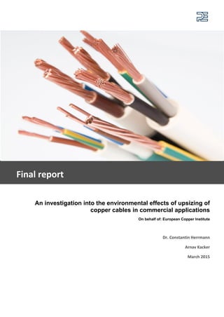
An investigation into the environmental effects of upsizing of
copper cables in commercial applications
On behalf of: European Copper Institute
Dr. Constantin Herrmann
Arnav Kacker
March 2015
Final report

This report has been prepared by PE INTERNATIONAL with all reasonable skill and diligence within the terms and conditions
of the contract between PE and the client. PE is not accountable to the client, or any others, with respect to any matters
outside the scope agreed upon for this project.
Regardless of report confidentiality, PE does not accept responsibility of whatsoever nature to any third parties to whom this
report, or any part thereof, is made known. Any such party relies on the report at its own risk. Interpretations, analyses, or
statements of any kind made by a third party and based on this report are beyond PE’s responsibility.
If you have any suggestions, complaints, or any other feedback, please contact PE at servicequality@pe-international.com.
Contact:
Dr. Constantin Herrmann
Arnav Kacker
Hauptstraße 111-115
Leinfelden-Echterdingen
70771 Germany
Phone +49 711 3418 17-0
E-mail
c.herrmann@pe-international.com
a.kacker@pe-international.com

3
TABLE OF CONTENTS
LIST OF FIGURES............................................................................................................................. 4
LIST OF TABLES .............................................................................................................................. 7
ACRONYMS ............................................................................................................................... 8
GLOSSARY (ISO 14040/44:2006) .................................................................................................. 9
EXECUTIVE SUMMARY................................................................................................................... 10
1 GOAL OF THE STUDY ............................................................................................................. 12
2 SCOPE OF THE STUDY ............................................................................................................ 12
2.1 Product System(s) to be studied ........................................................................................ 12
2.2 System Boundaries ............................................................................................................. 13
2.3 Cut-Off Criteria ................................................................................................................... 13
2.4 Selection of LCIA Methodology and Types of Impacts ....................................................... 14
2.5 Assumptions and Limitations ............................................................................................. 15
2.6 Software and Database ...................................................................................................... 15
2.7 Critical Review .................................................................................................................... 16
3 LIFE CYCLE INVENTORY (LCI) ANALYSIS..................................................................................... 17
3.1 Data Collection ................................................................................................................... 17
3.2 Product System................................................................................................................... 19
4 LIFE CYCLE IMPACT ASSESSMENT (LCIA) .................................................................................. 22
5 INTERPRETATION.................................................................................................................. 49
5.1 Identification of Relevant Findings..................................................................................... 49
5.2 Data Quality Assessment.................................................................................................... 49
5.3 Completeness, Sensitivity, and Consistency....................................................................... 50
5.4 Conclusions, Limitations, and Recommendations.............................................................. 50
6 REFERENCES........................................................................................................................ 51

4
LIST OF FIGURES
Figure 1: Global Warming Potential of Baseline vs. Economic scenario cables in large offices ...........11
Figure 2: Life cycle flowchart of the product system............................................................................19
Figure 3: Example GaBi plan for manufacturing of cables....................................................................20
Figure 4: Example GaBi plan for end-of-life of cables...........................................................................21
Figure 4-1: Contributions to the Acidification Potential of the manufacturing of the copper cable used
in small offices..............................................................................................................................23
Figure 4-2: Acidification Potential for the manufacturing and EoL of copper cables in a small office.24
Figure 4-3: Acidification Potential for the life cycle including the use phase of copper cables in a small
office.............................................................................................................................................25
in large offices ..............................................................................................................................25
Figure 4-5: Acidification Potential for the manufacturing and EoL of copper cables in a large office .26
Figure 4-6: Acidification Potential for the life cycle including the use phase of copper cables in a large
office.............................................................................................................................................26
in large industrial plants...............................................................................................................27
Figure 4-8: Acidification Potential for the manufacturing and EoL of copper cables in a large industrial
plant .............................................................................................................................................28
Figure 4-9: Acidification Potential for the life cycle including the use phase of copper cables in a large
industrial plant .............................................................................................................................28
Figure 4-10: Contributions to the Eutrophication Potential of the manufacturing of the copper cable
used in small offices .....................................................................................................................29
Figure 4-11: Eutrophication Potential for the manufacturing and EoL of copper cables in a small office
......................................................................................................................................................30
Figure 4-12: Eutrophication Potential for the life cycle including the use phase of copper cables in a
small office ...................................................................................................................................30
used in large offices......................................................................................................................31
Figure 4-14: Eutrophication Potential for the manufacturing and EoL of copper cables in a large office
......................................................................................................................................................31
large office....................................................................................................................................32

5
used in large industrial plants ......................................................................................................32
Figure 4-17: Eutrophication Potential for the manufacturing and EoL of copper cables in a large
large industrial plant ....................................................................................................................33
Figure 4-19: Contributions to the Global Warming Potential of the manufacturing of the copper cable
Figure 4-20: Global Warming Potential for the manufacturing and EoL of copper cables in a small office
......................................................................................................................................................35
Figure 4-21: Global Warming Potential for the life cycle including the use phase of copper cables in a
small office ...................................................................................................................................35
Figure 4-23: Global Warming Potential for the manufacturing and EoL of copper cables in a large office
......................................................................................................................................................36
large office....................................................................................................................................37
Figure 4-26: Global Warming Potential for the manufacturing and EoL of copper cables in a large
large industrial plant ....................................................................................................................38
Figure 4-28: Contributions to the Photochemical Ozone Creation Potential of the manufacturing of the
copper cable used in small offices ...............................................................................................39
Figure 4-29: Photochemical Ozone Creation Potential Potential for the manufacturing and EoL of
copper cables in a small office .....................................................................................................40
Figure 4-30: Photochemical Ozone Creation Potential Potential for the life cycle including the use
phase of copper cables in a small office ......................................................................................40
copper cable used in large offices................................................................................................41
copper cables in a large office......................................................................................................41
phase of copper cables in a large office.......................................................................................42

6
copper cable used in large industrial plant..................................................................................42
copper cables in a large industrial plant ......................................................................................43
phase of copper cables in a large industrial plant........................................................................43
Figure 4-37: Contributions to the Primary Energy Demand of the manufacturing of the copper cable
Figure 4-38: Primary Energy Demand (renewable and non-renewable) for the manufacturing and EoL
of copper cables in a small office.................................................................................................45
of copper cables in a small office.................................................................................................45
Figure 4-41: Primary Energy Demand (renewable and non-renewable) for the life cycle including the
use phase of copper cables in a small office................................................................................46
use phase of copper cables in a large office ................................................................................47
of copper cables in a large industrial plant..................................................................................48
use phase of copper cables in a large industrial plant.................................................................48

7
LIST OF TABLES
Table 2-1: System Boundaries...............................................................................................................13
Table 2-2: Impact Assessment Category Descriptions..........................................................................14
Table 2-3: Other Environmental Indicators ..........................................................................................15
Table 3-1: Key energy datasets used in inventory analysis ..................................................................17
Table 3-2: Key material datasets used in inventory analysis................................................................18
Table 3-3: Composition of the cables used in the scenarios small office, large office and large industrial
plant .............................................................................................................................................21
Table 4-1: Acidification Potential for the manufacturing and EoL of copper cables in a small office, large
office and large industrial plant ...................................................................................................23
Table 4-2: Eutrophication Potential for the manufacturing and EoL of copper cables in a small office,
large office and large industrial plant ..........................................................................................29
Table 4-3: Global Warming Potential for the manufacturing and EoL of copper cables in a small office,
large office and large industrial plant ..........................................................................................34
Table 4-4: Photochemical Ozone Creation Potential for the manufacturing and EoL of copper cables in
a small office, large office and large industrial plant ...................................................................39
Table 4-5: Primary Energy Demand (renewable and non-renewable) for the manufacturing and EoL of
copper cables in a small office, large office and large industrial plant........................................43

8
ACRONYMS
ADP Abiotic Depletion Potential
AP Acidification Potential
CML Centre of Environmental Science at Leiden
ELCD European Life Cycle Database
EoL End-of-Life
EP Eutrophication Potential
GWP Global Warming Potential
ILCD International Cycle Data System
ISO International Organization for Standardization
LCA Life Cycle Assessment
LCI Life Cycle Inventory
LCIA Life Cycle Impact Assessment
ODP Ozone Depletion Potential
PE PE INTERNATIONAL
POCP Photochemical Ozone Creation Potential

9
GLOSSARY (ISO 14040/44:2006)
ISO 14040:2006, Environmental management - Life cycle assessment - Principles and framework,
International Organization for Standardization (ISO), Geneva.
Allocation
Partitioning the input or output flows of a process or a product system between the product system
under study and one or more other product systems
Functional Unit
Quantified performance of a product system for use as a reference unit
Cradle to grave
Addresses the environmental aspects and potential environmental impacts (e.g. use of resources and
environmental consequences of releases) throughout a product's life cycle from raw material
acquisition until the end of life.
Cradle to gate
Addresses the environmental aspects and potential environmental impacts (e.g. use of resources and
environmental consequences of releases) throughout a product's life cycle from raw material
acquisition until the end of the production process (“gate of the factory”).
Life cycle
A unit operations view of consecutive and interlinked stages of a product system, from raw material
acquisition or generation from natural resources to final disposal. This includes all materials and
energy input as well as waste generated to air, land and water.
Life Cycle Assessment - LCA
Compilation and evaluation of the inputs, outputs and the potential environmental impacts of a
product system throughout its life cycle
Life Cycle Inventory - LCI
Phase of Life Cycle Assessment involving the compilation and quantification of inputs and outputs for
a product throughout its life cycle.
Life Cycle Impact assessment - LCIA
Phase of life cycle assessment aimed at understanding and evaluating the magnitude and significance
of the potential environmental impacts for a product system throughout the life cycle.
Life Cycle Interpretation
Phase of life cycle assessment in which the findings of either the inventory analysis or the impact
assessment, or both, are evaluated in relation to the defined goal and scope in order to reach
conclusions and recommendations.

10
EXECUTIVE SUMMARY
This study was commissioned to examine the environmental effects of the use of copper cables of
larger sizes in offices and industrial applications. Common opinion cites that the environmental impact
of production of additional copper makes the use of larger cable sizes environmentally
disadvantageous. In order to investigate this claim to a greater degree of detail and include the use-
phase implications of upsized cables, PE INTERNATIONAL conducted a comparative life cycle
assessment of standard cables against upsized cables. The study follows ISO14040/44 requirements
in its structure, quality on data, scope, and impact categories and it is ready for external review, which
would be necessary to reflect full conformity.
For the purposes of this study, three application locations have been considered: small offices, large
offices, and industrial areas. The definition of each of these application domains is available in the
report ‘Modified Cable Sizing Strategies’ by Egemin Automation /EGEMIN/, which this study builds
upon.
For the small and large offices, low voltage copper cables have been taken into consideration whereas
for industrial areas, where power demand is higher, medium voltage copper cables have been
considered. The amount of cable required for each of the three application cases is based upon the
copper demand specified in the Egemin Automation /EGEMIN/ report. This data is enhanced by
including the various layers of a cable (insulation, sheathing etc.). Using PE INTERNATIONAL’s
extensive and quality approved GaBi Databases and system modelling, the environmental impacts
associated with the cable production (including production of all inputs, up each branch of the supply
chain) have been quantified. The relative difference in power losses between standard cables and
upsized cables has been considered. The difference arises from the fact that cables with larger cross-
sectional area are subject to lower transmission losses. Lastly, at the end-of-life of the cables the
collection and recycling has been accounted for. The recycled metal and plastic components are used
in downstream material uses or energy generation through incineration. This downstream value takes
the form of an environmental credit in the system under consideration. The credit represent the
avoided burden of material or energy generation facilitated by the recycling of the product (cable).
Our study finds that in the production of the cable 60-90% of impacts result from the production of
the copper required for the cable with the rest coming from the production of the plastic components.
The exceptions to this range is the summer smog (photochemical oxidant creation potential, POCP)
impact category. 44% of POCP impact stems from copper production because plastic production
releases significant nitrogenous emissions that impact this category. It must, however, be noted here
that toxicity indicators have been deliberately excluded from analysis. These indicators are in a
nascent stage of development and yield contested results which are actively being debated in
European forums. It is generally recommended to avoid the use of toxicity indicators for
environmental decision-making without an in-depth discussion on inventory analysis and applied
method approval. This discussion is out of scope of this study and therefore toxicity results have not
been analysed in this report.
Extending the scope beyond production to include the entire life cycle (production, use, and end-of-
life), it becomes clear that within a few years of use the impact from the production of the cables is
overshadowed by the impacts due to energy losses. These impacts are represented by the emissions
associated with the production of the same quantity of energy in the European power grid mix.
The cables with smaller cross sections (Baseline scenario) have a lower starting (production) impact
but a greater annual energy loss rate. The upsized cables (Economic scenario), delivering equivalent
electrical function, have a higher starting (production) impact but a lower annual energy loss rate.

11
Therefore the cumulative impacts for different impact categories (acidification, global warming etc.)
intersect at a certain point before which the baseline scenario is advantageous and after which the
economic scenario is environmentally advantageous. A reference chart for the Global Warming
Potential in large offices is presented below.
Figure 1: Global Warming Potential of Baseline vs. Economic scenario cables in large offices
For the impact categories considered (acidification, eutrophication, global warming, summer
smog/ozone creation), this inflexion point lies before 1 year for all three application cases.
Overall, the environmental advantages of the upsized copper cables are apparent in our analysis. The
mitigation of increased production impact by use-phase savings is visible in the early inflexion point
(within 1 year compared to average cable lifetimes of about 30 years).

12
1 GOAL OF THE STUDY
The European Copper Institute (ECI) commissioned PE INTERNATIONAL to conduct an investigation
into the environmental implications of upsizing copper cables used in commercial applications in
Europe.
The commonly held view is that greater copper content is environmentally disadvantageous due to
the environmental impact of copper production. However, cables of larger sizes contribute to reduced
electricity losses. The goal of this study is to evaluate the reduced losses against the larger copper
production impact to investigate viability of copper upsizing from an environmental perspective.
This study builds on the findings of the EGEMIN study, ‘Modified Cable Sizing Strategies’ (2011). The
EGEMIN study specifies the copper cable content in the three commercial applications (small office,
large office and industrial plants) investigated in this study. Furthermore, the EGEMIN study also
quantifies the losses under the different cable sizes. These findings were to be used as a basis for the
environmental evaluation by PE INTERNATIONAL.
This study will be used by the ECI to present the case for copper upsizing to the internal (copper and
cable industry) stakeholders.
According ISO standards, in order to communicate the results externally (customers, LCA practitioners,
public in general, etc.) a critical review is mandated. At this stage, the results are not intended to be
used for communication disclosed to the public.
A critical review has not been conducted for this study.
2 SCOPE OF THE STUDY
The following section describes the general scope of the project to achieve the stated goals. This
includes, amongst others, the identification of specific product systems to be assessed, the functional
unit and reference flows, the system boundary, allocation procedures, and cut-off criteria of the study.
2.1 PRODUCT SYSTEM(S) TO BE STUDIED
The product system under consideration in this study is ‘Total copper cables used in the specified
commercial application’. The three commercial application cases considered are:
 Small offices
 Large offices
 Industrial plants
Low voltage copper cables have been used for the first two applications and medium voltage copper
cables for the industrial plants application case.

13
The quantity of cables used in each of these individual cases was specified in terms of the copper used
(EGEMIN study). This information was used by PE INTERNATIONAL together with bills of materials
provided by DNV-GL on behalf of ECI for the different cable types.
The cable consists of a core copper conductor, plastic isolation and additional layers such as swelling
tape and wire sheathing. All these materials have been accounted for in the model for this study.
The functional unit for this assessment is ‘Mass of copper cables required to provide electrical
demand of specific application case’.
2.2 SYSTEM BOUNDARIES
Table 2-1: System Boundaries
Included Excluded
 Raw materials
 Waste treatment
 Recycling impacts
 Environmental credits
 Use phase losses
 Capital equipment and maintenance
 Overhead (heating, lighting) of
manufacturing facilities when easily
differentiated
 Installation of cables
 Human labour
 Transports between all stages
2.2.1 Time Coverage
Foreground data is provided by DNV-GL, citing industry datasheets published in 2014 for low-voltage
cables and 2011 of the other products as well as through the results of the EGEMIN study. All
secondary data come from the Ga-Bi 2013 databases and are representative of the years 2009-2013.
As the study intended to compare the product systems for the reference year 2014, temporal
representativeness is warranted.
2.2.2 Technology Coverage
The technology mixes used are up-to-date for 2013 production of the respective materials. Further
details on the technological process mixes for the various materials is available in the GaBi
documentation online.
2.2.3 Geographical Coverage
The geographical scope of this project is the EU-27 region. Wherever available, European production
data has been used for the manufacturing of the raw materials. Where no relevant European data is
available, a suitable substitute has been used.
2.3 CUT-OFF CRITERIA
No cut-off criteria are defined for this study. All available energy and material flow data have been
included in the model.

14
2.4 SELECTION OF LCIA METHODOLOGY AND TYPES OF IMPACTS
A set of impact assessment categories and other metrics considered to be of high relevance to the
goals of the project are shown in Table 2-2 and Table 2-3. The CML impact assessment methodology
framework was selected for this assessment. The CML characterization factors are applicable to the
European context and are widely used and respected within the LCA community.
Table 2-2: Impact Assessment Category Descriptions
Impact Category Description Unit Reference
Global Warming
Potential (GWP)
A measure of greenhouse gas emissions, such as
CO2 and methane. These emissions are causing an
increase in the absorption of radiation emitted by
the earth, increasing the natural greenhouse effect.
This may in turn have adverse impacts on
ecosystem health, human health and material
welfare.
kg CO2
equivalent
[GUINÉE
2001]
Eutrophication
Potential
Eutrophication covers all potential impacts of
excessively high levels of macronutrients, the most
important of which nitrogen (N) and phosphorus
(P). Nutrient enrichment may cause an undesirable
shift in species composition and elevated biomass
production in both aquatic and terrestrial
ecosystems. In aquatic ecosystems increased
biomass production may lead to depressed oxygen
levels, because of the additional consumption of
oxygen in biomass decomposition.
kg Phosphate
equivalent
[GUINÉE
2001]
Acidification
Potential
A measure of emissions that cause acidifying effects
to the environment. The acidification potential is a
measure of a molecule’s capacity to increase the
hydrogen ion (H+) concentration in the presence of
water, thus decreasing the pH value. Potential
effects include fish mortality, forest decline and the
deterioration of building materials.
kg SO2
equivalent
[GUINÉE
2001]
Photochemical
Ozone Creation
Potential (POCP)
A measure of emissions of precursors that
contribute to ground level smog formation (mainly
ozone, O3), produced by the reaction of VOC and
carbon monoxide in the presence of nitrogen oxides
under the influence of UV light. Ground level ozone
may be injurious to human health and ecosystems
and may also damage crops.
kg ethene
equivalent
[GUINÉE
2001]

15
Table 2-3: Other Environmental Indicators
Indicator Description Unit Reference
Primary Energy
Demand (PED)
A measure of the total amount of primary energy
extracted from the earth. PED is expressed in
energy demand from non-renewable resources
(e.g. petroleum, natural gas, etc.) and energy
demand from renewable resources (e.g.
hydropower, wind energy, solar, etc.). Efficiencies
in energy conversion (e.g. power, heat, steam, etc.)
are taken into account.
MJ (net calorific
value)
[GUINÉE
2001]
It shall be noted that the above impact categories represent impact potentials, i.e., they are
approximations of environmental impacts that could occur if the emitted molecules would (a) actually
follow the underlying impact pathway and (b) meet certain conditions in the receiving environment
while doing so. In addition, the inventory only captures that fraction of the total environmental load
that corresponds to the chosen functional unit (relative approach).
LCIA results are therefore relative expressions only and do not predict actual impacts, the exceeding
of thresholds, safety margins, or risks.
2.5 ASSUMPTIONS AND LIMITATIONS
The limitations and assumptions associated with this LCA are listed below:
 The energy for the assembly of cables using the individual component materials has been
excluded from the analysis. This energy consumption represents a relatively small fraction of
net environmental impact and is not expected to skew the representativeness of the overall
results.
 The transport of the raw materials to the production site and the transport of the finished
product to the site of installation has not been accounted for. This impact is also relatively
small in relation to the net impact per functional unit.
 The packaging of the products has not been included in the scope of the manufacturing phase
of the products
 The effort of installation of cables is outside the scope of this study.
 An in-depth discussion or investigation of the applicability of available toxicity calculation
methods for facilitating comparability of the toxicity aspects from metals, plastics and grid
mixes lies outside the scope of this study.
2.6 SOFTWARE AND DATABASE
The LCA model was created using the GaBi 6 Software system for life cycle engineering, developed by
PE INTERNATIONAL AG. The GaBi 2013 LCI database /GaBi/ (documented at http://www.gabi-

16
software.com/support/gabi/gabi-database-2013-lci-documentation/) provides the life cycle inventory
data for several of the raw and process materials obtained from the background system.
2.7 CRITICAL REVIEW
No critical review has been conducted for this assessment. However the study follows the
ISO14040/44 requirements and is therefore ready for external review.

17
3 LIFE CYCLE INVENTORY (LCI) ANALYSIS
3.1 DATA COLLECTION
The data for the manufacturing phase of the cables was sourced from the DNV-GL report, ‘Typical
cables for input LCA’. This report specifies the bills of material for different types of copper cables –
high voltage, low voltage, medium voltage etc.
For the small and large office applications, low voltage cables have been taken into consideration. For
the industrial plant application, medium voltage cables have been considered. The data for the
quantities of cables required for the various applications has been sourced from the EGEMIN study
‘Modified Cable Sizing Strategies, 2011’.
The data on the end of life collection rates for the cable industry have been based off the findings of
the ECI market research consultant, Mr. Volker Schneider. Mr. Schneider interviews 8 cable recyclers
and scrap dealers in Europe to determine expert estimates on the recovery of cables after their service
lives. Furthermore, his findings provide a basis to determine the optimal recycling process through
which the recovered copper re-enters the production loops.
3.1.1 Fuels and Energy – Background Data
National and regional averages for fuel inputs and electricity grid mixes were obtained from the GaBi
6 database 2013. Table 3-2 shows the most relevant LCI datasets used in modelling the product
systems.
Table 3-1: Key energy datasets used in inventory analysis
* data were developed on-demand by PE for this specific project
3.1.2 Raw Materials and Processes – Background Data
Data for up- and downstream raw materials and unit processes were obtained from the GaBi 6
database 2012. Table 3-2 shows the most relevant LCI datasets used in modelling the product systems.
Documentation for all non-project-specific datasets can be found at www.gabi-
software.com/support/gabi/gabi-6-lci-documentation. /GaBi/

18
Table 3-2: Key material datasets used in inventory analysis

19
3.2 PRODUCT SYSTEM
3.2.1 Overview of Life Cycle
Figure 2: Life cycle flowchart of the product system
The life cycle of the product system considered in this study include the manufacturing of the cable
subcomponents. This entails quantifying all the impacts and emissions associated with the production
of the various cable parts such as the conductors, isolation sheathing etc.
For the use phase of the cables, this LCA includes the losses incurred per year of use of the cables in
each respective application case.
At the end of their serviceable lives, the cables are recovered and recycled. The rate of recovery and
efforts associated with the recycling of these products has been assessed in this study to estimate the
environmental credits to be accorded for the return of secondary material to the market (and
subsequent substitution of primary production.)

20
3.2.2 Description of Process Flow
3.2.2.1 Manufacturing
Figure 3: Example GaBi plan for manufacturing of cables
As seen in the figure above, the GaBi model for the manufacturing of the cables used in the respective
application cases quantifies the inputs and outputs of the production of the various cable
subcomponents. This study does not account for the energy required for the assembly of these
individual components into the final cable but this energy impact is considered to be small in relation
to the overall impact of the production of all the materials.

21
Table 3-3: Composition of the cables used in the scenarios small office, large office and large
industrial plant
Composition
[kg per m]
Small office
(low voltage cable)
Large office
(low voltage cable)
Large industrial plant
(medium voltage cable)
Copper 0.851 0.851 2.912
PE 0.000 0.000 0.505
Polyester 0.000 0.000 0.059
PVC 0.755 0.755 0.000
XLPE 0.052 0.052 0.569
3.2.2.2 Transport
No transport has been considered in the foreground system this life cycle assessment.
3.2.2.3 Use
The use phase losses associated with each cable system for each application case has been sourced
from the EGEMIN study. These losses have been simulated as an additional consumption of power
from the EU-27 Electricity Grid Mix.
3.2.2.4 End-of-Life
Figure 4: Example GaBi plan for end-of-life of cables
The figure above shows the GaBi plan for the end-of-life stage of the life cycle of a power cable. This
part of the model quantifies the collection rates (fraction of cables recovered from the ground after
cessation of service), the impacts from the recycling processes and associated material losses, and the
incineration and energy recovery during the recycling of the plastic fractions. Furthermore, the

22
recovered material and energy is granted an environmental credit to acknowledge the fact that these
recycled quantities substitute primary production on the market and thereby offset impacts that
would have otherwise occurred.
4 LIFE CYCLE IMPACT ASSESSMENT (LCIA)
The software model described above enables the calculation of various environmental impact
categories. The impact categories describe potential effects of the life cycle stages on the
environment. As different resources and emissions are summed up per impact category the impacts
are normalised to a specific emission and reported in “equivalents”, e.g. Greenhouse gas emissions
are reported in kg CO2 equivalents.
Environmental impact categories are calculated from “elementary” material and energy flows.
Elementary flows describe the origin of resources from the environment as basis for the
manufacturing of the pre-products and generating energy, as well as emissions into the environment,
which are caused by a product system.
A set of impact assessment categories considered to be of high relevance to the goals of the project
has been chosen. The CML (Center voor Milieukunde at Leiden, NL) impact assessment methodology
framework was selected for this assessment. The CML characterization factors are applicable to the
European context and are widely used and respected within the LCA community. The most recently
published list of characterisation factors “CML 2001 – Apr. 2013” has been applied.
Global warming potential and primary energy were chosen because of their relevance to climate
change and to energy and resource efficiency, which are strongly interlinked, of high public and
institutional interest, and deemed to be some of the most pressing environmental issues of our times.
Eutrophication, acidification, and photochemical ozone creation potentials were chosen because they
are closely connected to air, soil, and water quality and capture the environmental burden associated
with commonly regulated emissions such as NOx, SO2, VOC, and others.
Toxicity impact categories have been excluded from this study for the following reasons:
- The application of general toxicity criteria within the life cycle impact assessment (LCIA) of
metals, i.e. related to emissions of metal and metal compounds, currently poses significant
methodological and scientific problems as stated in the specific ILCD handbook. For metals,
the USEtox method does not consider some metal specificities (e.g. essentiality) or is highly
uncertain regarding the model parameters related to the long term behaviour, i.e. ageing, due
to their permanent character. Therefore, the USEtox characterization factors for metals are
rated as interim in the USEtox website and should then only be used with caution and not for
product comparison purposes.
- LCIA results for toxicity indicators are strongly impacted by the degree of development of the
LCI dataset since several thousands of substances are contributing to this impact
category. Therefore, the toxicity indicators are highly sensitive to the degree of completeness
of the LCI datasets not only for the foreground processes but also for all the background
processes. Hence, even if the quality of the LCIA methodologies is improving, the level of
completeness of the various LCI datasets is not sufficiently homogeneous to secure robust and
non-discriminatory results.

23
- For toxicity indicators, the PEF normalisation factors based on domestic European production
is largely underestimated compared to normalisation factors based on the European
consumption. Such underestimation is particularly significant for the indicators related to
toxicity and resource depletion. Hence, the contribution of USEtox indicators is largely
overestimated due to this inadequate choice of PEF normalisation factors.
It shall be noted that the above impact categories represent impact potentials, i.e., they are
approximations of environmental impacts that could occur if the emitted molecules would (a) actually
follow the underlying impact pathway and (b) meet certain conditions in the receiving environment
while doing so.
LCIA results are therefore relative expressions only and do not predict actual impacts, the exceeding
of thresholds, safety margins, or risks.
In fact, the results from the impact assessment are only relative statements, which give no information
about the endpoint of the impact categories, exceeding of threshold values, safety margins or risk.
The following information on environmental impacts is expressed with the impact category
parameters of LCIA using characterisation factors. Used method is CML 2001 (latest updated in 2013)
and USEtox.
4.1.1 Acidification Potential (AP)
Table 4-1: Acidification Potential for the manufacturing and EoL of copper cables in a small office,
large office and large industrial plant
AP
[kg SO2-equiv.]
Small office Large office Large industrial plant
Baseline Economic Baseline Economic Baseline Economic
Total 1.85 2.51 5.01 8.04 61.62 131.29
Manufacturing 2.39 4.40 10.58 19.79 171.04 388.59
EoL -0.54 -1.89 -5.57 -11.76 -109.42 -257.30
4.1.1.1 Small office
Figure 4-1: Contributions to the Acidification Potential of the manufacturing of the copper cable
used in small offices

24
In the Acidification Potential Category, 79% of the impacts from the manufacturing of raw materials is
associated with the production of the copper for the conductor. This stems mainly from the sulphur
dioxide emissions during the smelting and converting processes in the production of primary copper
cathode from ore. The plastic components of the cable (isolation, tape) contribute the remainder for
the AP impacts in manufacturing.
Figure 4-2: Acidification Potential for the manufacturing and EoL of copper cables in a small office
When looking at the manufacturing and end-of-life impacts together, it is seen that a significant
proportion of impacts are offset at EoL through credits. This is due to the fraction of copper that is
recovered and recycled and thereby ‘avoids the burden’ of production of primary copper when it re-
enters the market. To a smaller extent, these credits also account for the energy recovered from the
incineration of the plastic components from the recovered cables.
In the ‘Economic case’, with upsized copper cables, we see and larger impact from the production of
copper and a larger credit. The net value for the Economic Case is is higher than the Baseline when we
assess only the manufacturing and EoL stages. The chart below shows the life cycle impacts when we
take the effects of the use-phase losses into account as well.

25
Figure 4-3: Acidification Potential for the life cycle including the use phase of copper cables in a
small office
In the chart above, the time-scale is plotted on the X-axis while the AP impacts are on the Y-axis. At
the start of its life, each cable system is represented only by the net (manufacturing+EoL) impacts
from the previous chart. As the cable systems are used, the losses from the Baseline scenario
contribute quickly to higher cumulative losses than the Economic scenario, where upsized cables lead
to lower loss rates.
The high AP impact from the use-phase losses makes the manufacturing and EoL impacts almost
negligible. The greater net manufacturing impact of upsized cables in the Economic scenario is offset
in under 1 year of use, seen in the intersection of the orange and blue lines.
4.1.1.2 Large office
used in large offices

26
Since both small and large offices use low voltage cables, albeit in different quantities, the relative
contribution from the different components remains the same as in the previous application case –
79% from the production of the copper conductor and 21% from the plastic components of the cable.
Figure 4-5: Acidification Potential for the manufacturing and EoL of copper cables in a large office
large office

27
Similar to the application case for small offices, the net manufacturing impact (manufacturing+EoL) in
negligible to the scale of impact associated with the use phase losses. When comparing the Baseline
and Economic (upsized cables) scenario, the latter quickly offsets the greater production impact in
under a year.
4.1.1.3 Large industrial plant
used in large industrial plants
For industrial plants, larger medium voltage cables have been taken into consideration in this LCA.
With this bigger cables, the copper conductor has a higher share of the manufacturing stage impacts.
88% of total manufacturing impact comes from the conductor while 12% is from the plastic
components.

28
Figure 4-8: Acidification Potential for the manufacturing and EoL of copper cables in a large
industrial plant
large industrial plant
The large difference in loss rates between regular cables in the Baseline scenario and the upsized
cables in the Economics scenario ensure that the larger manufacturing impact is offset in a couple of
month and diverges greatly there on wards.

29
4.1.2 Eutrophication Potential (EP)
Table 4-2: Eutrophication Potential for the manufacturing and EoL of copper cables in a small office,
EP
[kg PO4
3-
-equiv.]
Total 0.12 0.19 0.41 0.71 5.00 10.95
Manufacturing 0.17 0.35 0.88 1.71 14.50 33.29
EoL -0.05 -0.16 -0.47 -1.00 -9.50 -22.34
Figure 4-10: Contributions to the Eutrophication Potential of the manufacturing of the copper
cable used in small offices
75% of the manufacturing phase EP impacts stem from the production of the copper conductor in the
cable systems. The plastic components contribute 25%.
These impacts are mostly associated with nitrogenous emissions from the production of the copper
conductor and the aluminium sheathing required for the low voltage cables.

30
Figure 4-11: Eutrophication Potential for the manufacturing and EoL of copper cables in a small
office
small office
The net manufacturing impacts are offset in under 1 year for the upsized cables due to the large
savings in use phase impacts.

31
cable used in large offices
office

32
large office
For large offices, the duration for the offset of manufacturing phase impacts is longer than that for
small offices but still under 1 year. Beyond that threshold the Economic scenario upsized cables are
advantageous in the EP category.
cable used in large industrial plants
For industrial plants, a greater share of the manufacturing stage impacts comes from the greater
copper conductor required for medium voltage cables. In this application case, 87% of the EP

33
contribution stems from the production of the copper while 13% is associated with the production of
plastics used in the cable construction.
industrial plant
large industrial plant
The payback of greater EP impacts for the upsized Economic case, through lower impacts for the use
phase, is less than 1 year for the industrial plant application case.

34
4.1.3 Global Warming Potential (GWP)
Table 4-3: Global Warming Potential for the manufacturing and EoL of copper cables in a small office,
GWP
[kg CO2-equiv.]
Total 547 921 2113 3822 21313 46702
Manufacturing 600 1107 2662 4980 37203 84068
EoL -53 -186 -549 -1159 -15890 -37366
Figure 4-19: Contributions to the Global Warming Potential of the manufacturing of the copper
In the GWP category, over 90% of the impacts for this category are associated with carbon dioxide
emissions at various stages of the life cycle.
These carbon dioxide emissions for low voltage cables are mostly through the production of the
copper conductor and through the production of the PVC isolation used.

35
Figure 4-20: Global Warming Potential for the manufacturing and EoL of copper cables in a small
office
Figure 4-21: Global Warming Potential for the life cycle including the use phase of copper cables in
a small office
The carbon dioxide emissions associate with the electricity losses are far higher than that associated
with the manufacturing of the upsized cables. As a result, the greater manufacturing phase impacts
due to upsizing the copper cables are offset in half a year. From that point onwards, all use of upsized
cables leads to a lower GWP over the life cycle compared to the regular cables of the baseline scenario.

36
The low voltage cables used for large offices have the same component contribution to GWP as in the
small offices application case.
office

37
a large office
The greater amount of cables required for large offices requires a longer payback period for GWP
impacts than in the case for small offices. In 1 year, the greater manufacturing GWp impact of upsized
low voltage cables in large offices is offset by use phase savings.
For the medium voltage cables used in aluminium plants, copper is the largest contributor to the GWP
impacts during the manufacturing phase, through the carbon dioxide emissions, followed by the
sheathing used.

38
industrial plant
a large industrial plant
The payback period for the larger GWP impacts for upsized cables in the Economic scenario is less
than half a year.

39
4.1.4 Photochemical Ozone Creation Potential (POCP)
Table 4-4: Photochemical Ozone Creation Potential for the manufacturing and EoL of copper cables
in a small office, large office and large industrial plant
POCP
[kg Ethene-
equiv.]
Total 0.15 0.28 0.66 1.22 5.80 12.75
Manufacturing 0.18 0.39 0.99 1.92 12.02 27.39
EoL -0.03 -0.11 -0.33 -0.70 -6.22 -14.63
Figure 4-28: Contributions to the Photochemical Ozone Creation Potential of the manufacturing of
the copper cable used in small offices
In terms of POCP impacts, it is not the copper but rather the PVC production that is the dominant
source of impacts with 56% of total contribution. It is chiefly the sulphur dioxide and nitrogen oxides
emission associated with the production processes that contribute to this category.

40
copper cables in a small office
phase of copper cables in a small office

41
the copper cable used in large offices
copper cables in a large office

42
phase of copper cables in a large office
As in the previous categories, the greater impact from upsized cables is offset within a year of their
use. Beyond this time frame of use, the upsized cables have a lower life cycle impact to this impact
category.
the copper cable used in large industrial plant

43
copper cables in a large industrial plant
phase of copper cables in a large industrial plant
4.1.5 Primary Energy Demand (renewable and non-renewable)
Table 4-5: Primary Energy Demand (renewable and non-renewable) for the manufacturing and EoL
of copper cables in a small office, large office and large industrial plant
PED
[MJ]
Total 9870 14471 30546 51600 349553 753084

44
Manufacturing 11367 19722 46013 84248 593005 1325582
EoL -1497 -5251 -15467 -32648 -243452 -572497
Figure 4-37: Contributions to the Primary Energy Demand of the manufacturing of the copper
For the production of low voltage cables used in offices, the copper is the dominant consumer of
primary energy in the manufacturing of the cable. The plastic isolation for these cables contributes
about 44% of the total manufacturing impact.

45
Figure 4-38: Primary Energy Demand (renewable and non-renewable) for the manufacturing and
EoL of copper cables in a small office
EoL of copper cables in a small office

46
Figure 4-41: Primary Energy Demand (renewable and non-renewable) for the life cycle including
the use phase of copper cables in a small office

47
the use phase of copper cables in a large office
4.1.5.3 Large industrial plants

48
EoL of copper cables in a large industrial plant
the use phase of copper cables in a large industrial plant
For all three application cases studied above, under the Primary Energy Demand impact category, the
payback of the greater net manufacturing impact from upsizing is offset within a year of use of the
upsized cables.

49
5 INTERPRETATION
5.1 IDENTIFICATION OF RELEVANT FINDINGS
 Upsized cables have a higher impact during manufacturing stage but these impacts are offset
by reductions in electricity losses
 For acidification, eutrophication, global warming, ozone creation and primary energy impact
categories, upsized cables result in lower net life cycle impact after 1 year of their use
 Following the 1 year mark, the upsized cables result in lower net impact level for the
aforementioned impact categories for each successive year of their use
5.2 DATA QUALITY ASSESSMENT
Inventory data quality is judged by its precision (measured, calculated or estimated), completeness
(e.g., unreported emissions), consistency (degree of uniformity of the methodology applied on a study
serving as a data source) and representativeness (geographical, temporal, and technological).
To cover these requirements and to ensure reliable results, first-hand industry data in combination
with consistent background LCA information from the GaBi LCI database were used. The LCI data sets
from the GaBi LCI database are widely distributed and used with the GaBi 6 Software. The datasets
have been used in LCA models worldwide in industrial and scientific applications in internal as well as
in many critically reviewed and published studies. In the process of providing these datasets they are
cross-checked with other databases and values from industry and science.
5.2.1 Precision and completeness
 Precision: As the relevant foreground data are primary data or modelled based on primary
information sources of the owner of the technology, no better precision is reachable within
this project.
 Completeness: Each unit process was checked for mass balance and completeness of the
emission inventory. See Section 2.5 for any omissions.
5.2.2 Consistency and reproducibility
 Consistency: All background data were sourced from the GaBi databases. Allocation and
other methodological choices were made consistently throughout the model. The sources
for the foreground data are the same for the Baseline and Economic scenarios studied here.
 Reproducibility: Reproducibility is warranted as much as possible through the disclosure of
input-output data, dataset choices, and modelling approaches in this report. Based on this
information, any third party should be able to approximate the results of this study using the
same data and modelling approaches.
5.2.3 Representativeness
 Temporal: The primary data were based on DNV-GL bill of materials compiled in 2014,
market research on recycling from 2014, and the EGEMIN study published in 2011. All
secondary data come from the GaBi 6 2013 databases. As the study intended to compare
the product systems for the reference year 2014, temporal representativeness is warranted.

50
 Geographical: As far as possible, primary and secondary data were collected specific to the
EU-27 region under study. Geographical representativeness is considered to be high.
 Technological: All primary and secondary data were modelled to be specific to the
technologies or technology mixes under study. Technological representativeness is
considered to be good.
5.3 COMPLETENESS, SENSITIVITY, AND CONSISTENCY
5.3.1 Completeness
All relevant process steps for each product system were considered and modelled to represent each
specific situation. The process chain is considered sufficiently complete with regard to the goal and
scope of this study.
5.3.2 Consistency
All assumption, methods, and data were found to be consistent with the study’s goal and scope.
Differences in background data quality were minimized by using LCI data from the GaBi 6 2013
databases. System boundaries, allocation rules, and impact assessment methods have been applied
consistently throughout the study.
5.4 CONCLUSIONS, LIMITATIONS, AND RECOMMENDATIONS
5.4.1 Conclusions
This study examines the environmental implications upsizing the copper cables used in three
application cases: small offices, large offices, and industrial plants.
These environmental impacts have been measured according to selected indicators that are
representative of environmental and health hazards.
This study finds that for the environmental impact categories of acidification, eutrophication, global
warming, ozone creation, and primary energy demand, the upsizing of copper cables is
environmentally advantageous. There is a greater impact associated with the production of these
larger cables but these are offset through the reduction in electricity losses. Since electricity
production based on the selected grid mix EU27 also contributes to the same impact categories,
reduced losses translates to environmental benefits. The longer the use of cables with lower loss rates,
the greater the environmental advantage in these impact categories tends to be. The difference in net
manufacturing impact (manufacturing + end of life) between regular cables in the Baseline scenario
and upsized cables in the Economic scenario is offset within 1 year of use for these impact categories.
Considering the widely accepted nature of the AP, EP, GWP, POCP and primary energy demand as well
as the high margin for error and instability in the toxicity evaluation methodologies, this study
concludes that, within the aforementioned scope of use and impact assessment, the upsized copper
cables (represented in the economic scenario) afford significant environmental benefits over the life
cycle of the cables.

51
6 REFERENCES
DNV-GL Typical Cables for Input LCA, DN-GL (on behalf of ECI), 2014
GUINÉE 2001 Guinée et al, An operational guide to the ISO-standards, Centre for Milieukunde
(CML), Leiden, the Netherlands, 2001
GABI GaBi Databases 2013 (http://www.gabi-software.com/support/gabi/gabi-database-
2013-lci-documentation/)
EGEMIN Modified Cable Sizing Strategies, Egemin Automation, 2011
ISO 14040 : 2006 ISO 14040 Environmental management – Life cycle assessment – Principles and
Framework, 2006
ISO 14044 : 2006 ISO 14044 Environmental management – Life cycle assessment – Requirements and
guidelines, 2006
PE INTERNATIONAL
2012
GaBi 6 dataset documentation, PE INTERNATIONAL AG, Leinfelden-Echterdingen,
2012
SCHNEIDER Market Research Report on recycling of cables in Europe, Mr. Volker Schneider (on
bahlf of ECI), 2014
VAN OERS 2002 van Oers et al, Abiotic resource depletion in LCA: Improving characterisation factors
abiotic resource depletion as recommended in the new Dutch LCA handbook, 2002

Environmental impact of economic cable sizing

Recomendados

Recomendados

Más contenido relacionado

La actualidad más candente

La actualidad más candente (20)

Similar a Environmental impact of economic cable sizing

Similar a Environmental impact of economic cable sizing (20)

Más de Leonardo ENERGY

Más de Leonardo ENERGY (20)

Último

Último (20)

Environmental impact of economic cable sizing