Local linear approximation

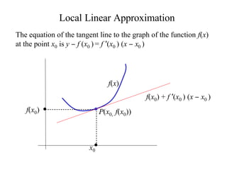
1. Local Linear Approximation
The equation of the tangent line to the graph of the function f(x)
at the point x0 is y − f (x0 ) = f ′(x0 ) (x − x0 )
f(x)
f(x0) + f ′(x0 ) (x − x0 )
f(x0)
P(x0, f(x0))
x0

2. f(x)
f(x0) + f ′(x0 ) (x − x0 )
x0
x
If x is close to x0, then the value of the function f(x) at x (the
height of the original curve at x), is very close to the value of the
function f(x0) + f ′(x0 ) (x − x0 ) at x, (the height that the tangent
line to f at x0 achieves at the point x).

3. ( ) ( )(
)
The function f x0 + f ′ x0 x − x0 is called the local linear
approximation to f at x0. This function is a good approximation
to f(x) if x is close to x0, and the closer the two points are, the
better the approximation becomes.
Example. Find the local linear approximation to the function
y = x3 at x0 = 1.
Solution.
( )
2
If f (x) = x3, then f ′(x ) = 3 x0 . Therefore,
0
2
x3 ≈ x 3 + 3 x0 x − x0 . If x0 = 1, then
0
x3 ≈1+ 3 x −1 = 3x − 2 for x close to 1.
( )(
( )
)

4. 3x - 2
x3
(1.01)3 =1.0303
3(1.01) −2 =1.03
(1.004)3 =1.01204
3(1.004) −2 =1.012
(0.997)3 =.991027
3(.997) − 2 = .991

5. Example. Find the local linear approximation to the function
1
y = at x0 = 2
x
Solution.
If f (x) = 1 , then f ′(x ) = −1 . Therefore,
0
2
x
( x0 )
(
)
1 ≈ 1 − 1 x − x . If x = 2, then
0
0
x x0 x 2
( 0)
(
)
1 ≈ 1 −1 x − 2 =1− x for x close to 2.
x 2 4
4

6. 1/x
1-x/4
1 =.4995
2.002
1− 2.002 =.4995
4
1 =.55075
1.997
1−1.997 =.55075
4

7. In practice, we use the idea of local linear
approximation in the following way.
1. We are given some value to calculate, say f(x), and the
calculation is difficult.
2. We see that there is a nearby point x0 where the
calculation of both f(x0) and f(x0)′ is relatively easy.
3. We approximate f(x) by f(x0)+ f(x0)′ (x − x0)

8. Example.Use local linear approximations to approximate the
quantity(1.98)3
Solution.
(a) A nearby point where the function x3 and its derivative are
easily evaluated is x0 = 2.
Near x0 = 2, the function x3 is approximated by the function
( ) ( )(
)
x0 3 + 3 x 0 2 x − x0 =8 +12( x − 2) =12x −16
Thus (1.98)3 is approximately 12(1.98) − 16 = 7.76
The true value is 7.762392.

9. Example.Use local linear approximations to approximate the
quantity 80.9
Solution.
(a) A nearby point where the function x and its derivative are
easily evaluated is 81.
Near x0 = 81, the function x is approximated by the function
(
)
x0 + 1 x − x0 = 9 + 1 ( x −81) = 9 + x
18
2 18
2 x0
Thus 80.9 is approximately 9 + 80.9 = 8.994444444
2 18
The true value is 8.994442729.

10. Example.Use local linear approximations to approximate the
quantity sin(.1) (.1 radians is about 5.7 degrees)
Solution.
(a) A nearby point where the function and its derivative are
easily evaluated is 0.
Near x0 = 0, the function sin(x) is approximated by the function
(
)
sin(x ) + cos(x ) x − x0 = 0 +1( x −0) = x
0
0
Thus sin(.1) is approximately 0.1.
The true value is .099833.

11. Approximating Changes - Differentials
The second use of the derivative is to approximate small
changes in a function. Start at a point x and move a small
distance given by the independent variable ∆x. Then define ∆y
to be the corresponding change in the value of y = f(x). We see
that ∆y = f(x + ∆x) – f(x).
y + ∆y = f(x +∆x)
∆y
y = f(x)
x + ∆x
x
∆x

12. Now let us move away from x another small distance given
by the independent variable dx, and define the dependent
variable dy to be the corresponding change of the height of
the tangent line at x. Then dy = f′(x)dx
dy
f(x)
x
x + dx
dx

13. Definition. Let dx be an arbitrary variable, and define dy to
dy .
be f ′(x)dx. Then the ratio of dy to dx is the derivative
dx
dx and dy are called differentials.
If we set dx = ∆x and combine the two diagrams, we see that dy
is a good approximation to ∆y when ∆x is small.

14. y + ∆y = f(x + ∆x)
y = f(x)
∆y
dy
y = f(x)
x + ∆x
x
dx = ∆x

15. Example. Find an expression for dy for each of the following
functions:
(a) f(x) = x4
(b) f ( x) = x
(c) f(x) = sin(x)
Solution.
(a) dy = d[x4] = (4 x3)dx
(c ) dy = d[sin(x)] = cos(x)dx
(b) dy = d[ x ] =  1  dx
2 x 


Example. (a) Find the differential dy if y = x−17
(b) What is dy when x = 1?
Solution. (a) dy = (−17)x−18dx
(b) dy = (−17)dx

16. Example. Let
y = 2 + 2x
let x = 2, and let dx = ∆x = 0.1. Compute dy and ∆y.
Solution.
(
∆y = f ( x +∆x) − f (x) = f (2.1) − f (2)
)(
)
= 2 + 4.2 − 2 + 4 ≈ 4.049 − 4 =.049
On the other hand
dy = f ′( x)dx = 1 dx = 1 (.1) =.05
2
2x

17. Example. Let y = x 2 +8 . Use dy to approximate ∆y when
x changes from 1 to 0.97
Solution. Here x0 = 1, and dx = ∆x is 0.97 –1 = – 0.03.
 x2 +8 ′
 2 ′
 dx = 2 x dx = x dx


dy =  x + 8  dx = 


2 x 2 +8
2 x 2 +8
x 2 +8
At x = 1, we have
dy = 1 dx = 1(−.03) =−.01
3
3
[The true value of ∆y is (.97)2 +8 − 9 =−.009866

18. Example. Let y = x 8x +1 . Use dy to approximate ∆y when
x changes from 3 to 3.05
Solution. Here x = 3, and dx = ∆x is 3.05 –3 = 0.05.

′
4x 
 8


dy =  x 8x +1  dx =  8x +1 + x
dx =  8x +1 +

 dx


8x +1 
 2 8x +1 


12 

At x = 3, we have dy = 25 +
dx = 37 (.05) =.37

25 
5


The true value of ∆y is
3.05 8(3.05) +1− 3 25 =15.372 −15 =.372

19. Example. A metal rod 15 cm. Long and 5 cm. in diameter is to
be covered (except for the ends) with insulation that is
0.001 cm thick. Use differentials to estimate the volume of
insulation needed.
Solution. Let V be the volume of the rod, R the radius, and L
the length.
Then V =π R2L. Thus dV = 2π RLdR
We estimate the volume of insulation to be the change in the
volume of the cylinder when its radius changes from 2.5 cm.
to 2.501 cm., that is dR = .001 cm.
Then dV = 2π RLdR = 2π (2.5)(15)(.001) ≅ 0.236cm3

20. Estimating Errors in Computations
Suppose that some quantity x is measured in an experiment.
There is always the possibility that the measurement is in
error to some extent, and the maximum amount of such error
is often specified in the literature that accompanies the
measuring device or program.
Frequently a computation is performed on the measured
value x, producing the result f(x). The question is:
What is the maximum error present in the computed
quantity f(x)?

21. Suppose that the maximum error in a measurement x is known to
be ∆x. We reason as follows:
Suppose that the true value of the quantity measured is x0. Then
the distance between x and x0 is no more than ∆x, and therefore
the maximum error in the computed value f(x) is estimated by
f(x0) − f(x) = f(x + ∆x) − f(x) = ∆y. We approximate this by dy.
In general we know the magnitude of the maximum
measurement error, but not the sign. Thus we use the symbol ±
in front of errors.

22. Sometimes, instead of estimating the absolute error, we are more
interested in the relative errors
dx and dy = d [ f (x )]
y
f ( x)
x
If these are multiplied by 100 to express them as percents, we
call them the percentage errors.If we are given the maximum
percentage error of the measurement, then we want to estimate
the maximum percentage error in the computed result.

23. Example. The side of a cube is measured to be 25 cm. With a
possible error of ± 1 cm.
(a) Use differentials to estimate the error in the calculated
volume.
(b) Estimate the percentage errors in the side and volume.

24. Example. The side of a cube is measured to be 25 cm. With a
possible error of ± 1 cm.
(a) Use differentials to estimate the error in the calculated
volume.
(b) Estimate the percentage errors in the side and volume.
Solution. (a) Let s stand for the length of the side of the cube,
and V stand for the volume. Then we know that
V = s3
It follows that dV = 3s2ds. The measured value of s is 25,
and we are given that the maximum value of ds is ± 1.
Thus
dV = 3(25)2 (±1) =±1875cm3.

25. Solution. (b) The relative error in measurement is
ds = ±1 =±.04
s 25
which is ± 4 percent.
The relative error in the computed volume is therefore
dV = 3s 2 ds = 3ds = 3(± .04) =±.12 Or 12 percent.
V
s
s3

26. Example. The electrical resistance of a certain wire is given by
R= k
r2
Where k is a constant and r is the radius of the wire. Assuming
that the listed radius r has a possible percentage error of
±5%, use differentials to estimate the percentage error in R
(assume k to be exact.)
Solution. dR = −2k dr
r3
Since
dR = r 2 × −2k dr =−2dr
so
R k r3
r
dr
dR
is ±5%,
is ±10%.
r
R

27. Example. The area of a circle is computed from the measured
value of its diameter. Estimate the maximum permissable
percentage error in the measurement, if the percentage
error in the area must be kept within ±1%.
π D 2 . Thus dA = π D dD
Solution. A =π R2 =
4
2
so dA = 4 ×π D dD = 2 dD
A π D2 2
D
If dA is to be less than or equal to ±1%, it follows that the
A
maximum value for dD is ±.5%.
D