1. Contents
1) Introduction………………………………………………………………………………………….2
2) Optimisation flow diagram………………………………………………………………………….3
3) Daily Counters………………………………………………………………………………………4
3.1 Call Set up Success Rate………………………………………………………………………4
3.2 High Dropped Call Rate……………………………………………………………………..11
3.3 High Handover Failure Rate……………………………………………………………...….17
3.4 SDCCH Blocking……………………………………………………………………...…….19
3.5 TCH Blocking……………………………………...………………………………………...20
3.6 SDCCH Mean Holding Time……………………………………………...………………...21
3.7 Erlangs……………………………………………………………………………...………..21
3.8 Total Calls……………………………………………...……………………………...……..21
4) Weekly statistics…………………………………………………………………………………...22
4.1 Traffic Trend……………………………………………………………………...………….22
4.2 Cell Retaining…………………………...…………………………………………………...23
4.3 Cell Accessibility……………………………………...……………………………………..24
5) Monthly statistics…………………………………………………………………………………..26
5.1 Processor load………………………………………………………………………….….…26
5.2 Call Success Rate………………………………………………………………...…………..27
5.3 Handover Success Rate………………………………...…………………………………….29
6) Reports……………………………………………………………………………………………..31
6.1 BSC capacity Report………………………………………...……………………………….31
6.2 BSC performance Report……………………………………………...……………………..32

2. INTRODUCTION
This document describes in the process of optimisation in GSM900/1800 mobile telephone systems.
The document covers the traditional methods of optimising a cellular system in the basic optimisation
section. It introduces the improvements being made to Aircom’s Optimisation process with the
introduction of new tools and techniques in the advanced optimisation section. Aircom has a tool
namely “ optima ” to monitor the system performance. A series of counters are monitored on daily,
weekly and monthly basis to check the network health. The document will specify the recommended
metrices and the standard performance management procedures to identify and rectify the problems
.
Optimisation is an invaluable element of service required to maintain and improve the quality and
capacity of a network. It is essential if an operator wants to implement changes to the network to
maintain the high quality of service levels expected by subscribers in GSM900/1800 networks. Without
optimisation the network will degrade from the commissioned state, due to the network changing
radically as the traffic on the GSM system grows, and snapshot optimisation will not keep pace with
these changes. Without optimisation the system will suffer poor call quality, many dropped calls due to
interference and inaccurate parameters resulting in poor handover performance. These together with
other problems, have the same result, Subscriber Dissatisfaction.
Setting the parameters that control mobility has equal importance to the frequency plan. In
GSM900/1800 networks there is a series of parameters that control mobility. Tuning these parameters
for improved GSM900/1800 operations, in terms of maximising calls carried, improved handover
performance and increased call success rate, is termed ‘Optimisation’.
The aim of optimisation is to maximise the Quality of Service (QoS) of the GSM network. In order to
do this you need to measure the QoS, compare the measured value with the desired value, and then take
steps to correct the causes of any deviations from the desired value.

3. INPUTS PROCESS OUTPUTS
RF DESIGN
PROCESS
QUALITY OF INTERGRATION OF
SERVICE METRICS SYSTEM OR NEW FREQ.
PLAN
DATABASE
PARAMETERS OPTIMISATION
OPTMISATION REPORT
RF DESIGN
PARAMETERS
OMC
DRIVE TEST
ROUTES
APPROX 2 - 4 WEEK PROCESS
PERFORMANCE PERFORMANCE
ENGINEERING REPORT
SYSTEM
ACCEPTANCE
FIGURE 2.1 Basic Optimisation Process
The flowchart shown in figure 2.1 summarizes the basic optimisation process.

4. 3. Daily Counters:
The following metrics can be used to measure the performance of the network. These counters should
be monitored daily on a per cell basis. These counters are defined in Optima under the heading of “
cell statistics ”.
S.NO Daily Counters to Monitor Standard Thresholds
1 Call set up success Rate Below 90 %
2 Tch Congestion Greater than 2%
3 Sdcch Congestion Greater than 2 %
4 Handover Success rate Below 85 %
5 TCH Drop Rate Greater than 2 %
6 TCH blocking Greater than 2 %
7 SDCCH blocking Greater than 2 %
8 Erlangs per hour -
9 Average no of TCH’s available -
10 Total Calls -
3.1 Call Setup Success Rate:
The call setup rate should be above 90 % for a healthy network. However a CCSR of 85%-90% is
satisfactory. Within optima the PSFAIL displays the percentage of call set up failure rate. There could
be so many reasons for a poor CSSR. Some are described as follows.
a) No Access to Sdcch
b) CM service reject
c) Tch Failure assignment
d) Hardware Problems
a-)No Access to SDCCH:
BSS detects Channel Request (in the form of RACH) from a source, requesting resources for network
transactions. After validation of the RACH, BSS will attempt to allocate a dedicated channel (SDCCH)
for the source. Once the availability of SDCCH channel is confirmed, the BSS will send Immediate
Assignment to MS indicating the dedicated SDCCH sub-channel (via AGCH), whereby subsequent
message exchange will be performed over the dedicated SDCCH.
Examples of Abnormality:
1-) Valid RACH (SDCCH Congestion)
Due to the unavailability of SDCCH, BSS will response to MS with Immediate Assignment
Reject, terminating the transactions. In which case, call setup is termed as unsuccessful due
to SDCCH congestion

5. Optimisation tips:
Within the optima there are certain statistics which can be monitored before concluding that there is
SDCCH problem
1-) PCFAIL
2-) PCCONGS
3-) CTCONGS
4-) CNDROP
“ PCFAIL ” represents the percentage of Control channel set up failure and “ PCCongs ” indicates the
percentage of Control channel congestion. In the figure cell statistics have been shown. Three different
thresholds have been defined for performance counters. These will show up in different colours in the
cell statistic window so that you can easily see which cells go above or below the value. In the fig Red
colour is peak threshold for any counter. Considering the site “ Mowbray house ”(site 15Aas shown in
fig 1and fig 2) where the percentage control channel failure exceeds the threshold (3.71 %), the
possible reason for higher failures could be control channel congestion. On observing PCCONGS it
comes out to be 8.13 % which is reasonably a higher value.
“Ctcong” is another counter to look at while monitoring the control channel congestion. When the last
available channel is allocated the congestion time counter is incremented each second until a channel is
idle. The value for Ctcong is 184, which is again a good indication of SDCCH blocking.
If the SDCCH congestion is greater than 2% than that means that it is a capacity related issue and more
slots should be assigned for SDCCH. A sudden high rise in congestion can also be understood by
analysing the neighbour’s performance. If there is a hardware failure or failures on TCH in the
neighbouring cell, most of the calls will be handed over to other cells increasing the overall floor of
congestion.
A Tch can be allocated bypassing Sdcch. A parameter namely Immediate_assign_mode when enabled
allocates Tch bypassing SDCCH.

6. Fig.1 Table presenting the Cell counters for the last hour. ( site 15 A showing 3.71%
Pcfail )
Fig 2. Table presenting the Cell counters for the last hour. (PCCONG for the Mowbray house is
8.13% showing SDCCH Congestion

7. 2-) Phantom RACHs
The received RACH is in fact generated from an “unknown source”, whereby it fails to continue the
transactions after SDCCH has been allocated by the BSS. For instances, cases of Channel Request
detected by over-shooting cells, Handover Access burst from distanced MS, hardware deficiency,
UL/DL imbalance path, MS moving out of range would carry the Phantom RACHs symptoms. fig 3
showing PRFAIL ( percentage of rach failure ) for site 36c.
FIG 3 (Site 36C with PRFAIL of 28.32 percent)
b-)CM Service Reject:
CM Service Request [MOC] or Paging Response [MTC] to BSS/MSC. Inside the CM Service Request
message (MS initiated service request), MS informs the network the types of services it requires (i.e.
Mobile Origination Call, Emergency Call, Short Message Transfer or Supplementary Services Activity.
MSC will response with either Connection Confirmed, confirming the success in link establishment
between MS-BSS-MSC, or Connection Refused, indicating the termination of the specific network
transaction.
Examples of Abnormality
1. Basically, the generation of excessive Connection Refused messages could relate to MSC
internal issue.
Upon successful link establishment, a number of signalling activities will proceed. Firstly,
Authentication Request will be sent to MS followed by cipher mode command. Thirdly, MSC will send
Identity Request to MS, questioning the IMSI. MS should response with its IMSI in the Identity

8. Response message to MSC for validation. MS-BSS-MSC connection will be cleared down if any of the
above three signalling activities fail. In general, Authentication Request, Cipher Mode Command or
Identity Request does not always appear during call setup, the occurrences of the three signalling
activities is controlled by MSC. (e.g. Authentication Request is only performed on every 10th
call in the
network)
.
Examples of Abnormality
1. MS related (e.g. incompatibility in ciphering algorithm, identity, etc)
C-)TCH Failure Assignment:
Upon completion of MS/BSS/MSC link establishment, MSC issues Assignment Request to BSS,
requesting TCH assignment to the dedicated MS. Subsequently, BSS will attempt to allocate free TCH
for MS voice messaging. Once Assignment Command is received by MS, stating the availability of
TCH for the MS, it will move to the dedicated TCH and responds with Assignment Complete. In turns,
BSS will submit Assignment Complete to MSC as to complete the signalling activity.
Examples of Abnormality
a-) TCH Congestion
BSS responses to MSC via Assignment Failure, indicating the unavailability of TCH
resources. BSS will subsequently terminate all transactions, in which case, call setup is
termed as unsuccessful due to TCH congestion.
b-) Interference on TCH
There could be co-channel or adjacent channel interference on a particular TCH causing
TCH failure assignment.
Optimisation tips:
For TCH congestion certain features can be enabled like TCH queuing, Directed Retry and Congestion
Relief.In the case of TCH Queuing feature is enabled, MS will queue in the original SDCCH, awaiting
for the next available TCH. It is to be reminded that once Queuing Timer expires, BSS will also
terminates all transactions, in which case, call setup is termed as unsuccessful due to TCH congestion.
The same situation also applies in situation where Congestion Relief feature is enabled.
In the case of Directed Retry feature is enabled, MS will perform handover to TCH of another cell if a
valid handover neighbour is detected. The best thing to do is to add more radios in the cell to remove
congestion.
Interference analysis on a particular carrier can be done through an optimisation tool like Neptune.
Once interfering frequencies are determined, the frequency plan can be cleaned from such frequencies.
Considering the example of Westlodge (site 20 B shown in fig 4) where call set up failures (23.4%)
have been affected due to traffic channel congestion (8.21 %).

9. Fig 4 .(Site 20b having high Pcong )
Mitchells Plain (cell site 36 C) is a classical example of call failure rate affected due to the interference
(PU5 indicates the percentage of ideal channel measurement in the fifth band)

10. Fig 5 (Cell site 36C showing call set up failure rate due to interference problem)
Hardware Problems:
Hardware failures also play the major role for Poor CSSR. Improper functionality of any BTS
hardware can affect the overall performance of site
Optimisation Tips:
If there are no capacity or RF issues then equipment needs to be checked. Before starting the drive test
make sure that the cell sites are free of any hardware alarms. The important parameter to check is the
Path balance. If Path balances are not fine then start checking the power from radio to connected
antennas. If we take the example of GSM 900 scenario, the link budget defines that the radio should
transmit 40 watts power and at the top of the cabinet, 20 watts are received (considering the 3 dB loss
of combiner). while checking the power, if any components seems to produce more losses than
expected, change that component. Similarly check the power at antenna feeder ports. Some time due to
the water ingress, connectors get rusty and needs to be replaced.

11. 3.2 High Dropped Call Rate:
For a healthy network the drop call rate should be less than 1 %. There are again number of reasons,
which could contribute towards higher dropped call rate.
a-) Drop on Handover
b-) low signal level / quality
c-) Adjacent channel / Co-channel interference
d-) Extraneous interference
f-) link imbalance
a-) Drop on Handover
The call may drop on handover. It’s mostly high neighbor interference on the target cell, which causes
the main problem. Sometime the mobile is on the wrong source cell (not planned for that area but
serves due to the antenna overshoot) which may result in the call drop.
Looking closely at site 256A (L’aubade) % age drop rate for tch is 2.13 ( fig 6) whereas there are
larger no of handovers on uplink quality clearly indicating the issue of interference. Closely looking at
Cell history the graph shows that there is high call drop rate also.
Fig 6. (Cell site 256 A showing more handovers on uplink quality)

12. Fig 7. ( Cell History graph showing percentage drop call rate )
Fig 8. (Ptfail is also high for 256 A)

13. Optimisation Tips:
Within optima, monitor the following statistics. Theses statistics are defined under the category of
BSC level statistics.
1-) Total and successful handovers on up/dl quality.
2-) Total and successful handovers on up/dl signal strength.
3-) Total and successful power budget handovers.
From the above statistics, quality or level issues can be estimated. If there are more handovers on
uplink and downlink quality then it is truly an indication of interference issues. In a good network there
should me more Power budget handovers than quality and level handovers.
b-) Low Signal Level / Quality
Signal level below –95 dbm is considered to be poor. If the mobile is unable to handoff to a better cell
on level basis, the call will possibly be dropped. Topology or Morphology issues may also be there like
if Mobile enters into a tunnel or a building, higher RF losses will be developed.
Optimisation tips:
The statistic which could be useful in assessing the drop calls on signal strength is “ DisBSS ” which
shows the number of disconcertion due to bad signal strength. Site “ Koeberg hill ”( fig 9) as indicated
has Percentage drop call rate of 3.1 %. Total number of disconnection failures due to bad signal
strength is 411, which clearly indicates the severe receive level problem.

14. Fig 9. ( site 130 A has large disconnection failure on bad level )

15. Fig 10. (Showing the quality and level problem in Harare Police station site 967 B)
First of all Path balances should be checked. If Path balances are deviating form the standard value
than Check the BTS transmitted power with the help of wattmeter. BTS may transmit low power
because of the malfunctioning of radio or higher combiner losses. Also check the feeder losses, antenna
connectors. Enable downlink Power Control. Power control is bi directional. The lower and upper
receive level downlink power control values should be properly defined.
1-) l_ rxlev_ dl_p
defines the lower value for receive level for the power control to be triggered .
Range = 0 to 63
Where 0 = -110 dbm

16. 1 = -109 dbm
63 = -47 dbm
e.g if the value of 20 is set it means that the BTS will start transmitting more if it senses that downlink
receive level is below –90 dbm.
2-) u_rxlev_dl_p
defines the upper threshold value for receive level for the power control to be triggered. (Range is same
as described above)
e.g on setting the value of 50 ( equivalent to –60 dbm ) BTS will lower down the power .
c-) Adjacent and Co Channel Interference
Frequency planning plays a major role to combat adjacent channel and Co channel interference. Co
channel is observed mostly when mobile is elevated and receives signals from cell far away but using
the same frequencies.
Taking into consideration the cell site 681A( fig 11) where there is a severe amount of interference
(PU5 indicating 100 percent). The cells where high amount of interference is observed are usually
affected by external interference.
FIG 11. ( Cell site 681A showing large amount of interference)
Optimisation tips:
An optimisation tool like Neptune could be helpful in identifying the interference on a particular area.
Such frequencies can be cleaned form existing frequency plan. The following statistics can also be
monitored to confirm that there are interference issues in the cell. These stats are defined in optima
under the category of BSC stats.

17. 1-) TCH interference at level 1
2-) TCH interference at level 2
3-) TCH interference at level 3
4-) TCH interference at level 4
When a tch timeslot is idle it is constantly monitored for an uplink ambient noise. During a SACCH
multiframe an idle time slot is monitored 104 times. These samples are then processed to produce a
noise level average per 480 ms. An interference band is allocated to an idle slot depending upon the
interference level. The thresholds for these levels can be set in the system parameters, interference level
1 being the least ambient and interference level 4 being the most ambient. While planning the network
care should be taken that the cells do have the proper frequency spacing.
d-) Extraneous Interference
Extraneous interference might be from
• Other mobile networks
• Military communication
• Cordless telephones
• Illegal radio Communication equipment
Optimisation tips:
External interference is always measured through spectrum analyser which can scan the whole band.
Some Spectrum analyser can even decode voice from AMPS circuits or Cordless Phones.
e-) Link Imbalance
Some time the malfunctionality of vendor hardware becomes responsible for high call drops. One of
the possible scenarios could be
• Transmit and Receiving antenna facing different direction
• Transmit and Receiving antennas with different tilts
• Antenna feeders damage, corrosion or water ingress
• Physical obstruction
3.3 High Handover Failure rate:
High Handover failures rate will probably be due to one or more of the following reason.
a-) High Neighbour Interference/ Congestion
b-) No Dominant Server
c-) Database Parameters
d-) Link Imbalance

18. a-) High Neighbour Interference/Congestion
While handing off to the best neighbour the interference on the target cell frequency may result in the
hand off failure. Neighbour Congestion is another issue, which can be looked at to assess handover
failures.
Optimisation tips
When designing the cell frequencies care should be taken that there is proper frequency spacing
between the cells to avoid neighbour interference. In most of the cases Ping pong Handover starts i.e
the mobile hand off to a cell for better level and due to interference (quality issues) hand off again to
original cell. A thorough drive test can determine the “interfering frequencies” which should be
eliminated from the frequency plan.
b-) No Dominant Server
If cell sites are designed poorly there might be areas where neighbour being received at the same level
and some neighbours randomly look good for handoff for a certain amount of time. Such situation is
disastrous because handoff decision will be hard and mostly it will end up in unsuccessful handovers.
Optimisation tips
Antenna tilts provide the good way to reduce the footprint of the sites. Efforts should be made that a
single dominant server should serve the specific area. Timing advance limitation ( ms_max_range) is
applied to cell areas where there is multiple servers.
c-) Database parameters
Received level, receive quality and Power budget algorithm are set in the system information to define
the criteria for Handover. Improper values for these criteria may result in poor handoff.
Optimisation Tips
Enable the “ Per neighbour ” feature which displays the successful and unsuccessful handovers on a
per cell basis. In “optima ” monitor the following stats, which comes under “ cell statistic category ”.
HOCNT (handover count from source cell to destination cell over reading period)
HOSUCC (Success Count from source cell to destination cell over reading period)
HORET (Returned Count from source cell to destination cell over reading period)
HODROP (Dropped count from source cell to destination cell over reading period)

19. All those cells can be identified which are problematic in terms of hand off so one can focus only
specific cells causing the major contribution towards poor HSSR. Ensure that handover margins are
optimised. Rule of thumb is 4 dB for adjacent frequencies and 6 dB for cell without adjacent
frequencies. The following parameters can be played for defining the thresholds for imperative and
non-imperative handovers.
1-) l_rxqual_up_h (defines the lower threshold for uplink quality handover)
Range: 0 to 1800
Step size: 0.01
e.g. a value of 500 defines the lower threshold value of 5( BER ) for a quality handover to be
triggered for uplink. The optimum value for this threshold is 500
2-) l_rxqual_dl_h (defines the lower threshold for downlink quality handover)
3-) l_rxlev_up_h (defines the lower threshold for received level uplink handover)
e.g. a value of 20 defines the threshold value of -90 dbm for a level handover to be triggered for
uplink.
Range: 0 to 63
Where 0= -110 dbm
1= -109 dbm
47= -63 dbm
The optimum value for this threshold is 15 i.e. 95 dbm. If the signal level goes below that, a level
handover is initiated.
4-) l_rxlev_dl_h (defines the lower threshold for received level downlink handover)
5-) u_rxlev_dl_ih (defines the upper threshold for downlink interference hand over)
6-) u_rxlev_dl_ih ( defines the upper threshold for uplink interference Handover )
3.4 SDCCH Blocking
SDCCH blocking is probably due to one or more reasons.
a-) No access to SDCCH
b-) Failure before assignment of TCH

20. c-) High Paging load
d-) Incorrect or inappropriate timer values
The first two reasons has already been discussed.
c-) High Paging load
Irregular paging distribution in location areas results in SDCCH blocking. Higher paging load in
certain location area means higher location updates on SDCCH resulting in SDCCH blocking.
Optimisation Tips:
A location area with a high paging load needs to be reduced in size to relieve SDCCH blocking. A
location area with a low paging load needs to be enlarged in size to reduce the overall number of
location areas.
d-) Incorrect or inappropriate timer values
Timer rr_t3 111 sets the amount of time allowed to delay the deactivation of a traffic channel (TCH)
after the disconnection of the main signalling link.
Optimisation Tips:
The suitable value for this timer is 1200 ms (max being 1500 ms). The timer will cause the BSS to wait
before the channel in question is allocated another connection. A lower value of timer will result in
higher capacity since the channel is held for less time before being released.
3.5 TCH Blocking:
Tch blocking may be due to the following reasons
a-) Handover and Power budget margins
c-) Cells too large
d-) Capacity Limitations ( congestion )
e-) Incorrect or appropriate timer
a-) Handover Margin
Handover margins should be properly optimised to move the traffic to neighbouring cell. Strict
handover margins can result in lower handovers and ultimately congestion in cell
Optimisation tips

21. 6 db handover margin is considered to be an appropriate margin for handover. A strict handover margin
results in the strict criteria for Power budget handovers also. Setting a lower value of handover margin
will initiate ping-pong handovers, which are not considered good for network health. ( hand over
margins have already been discussed )
b-) Cells too large
If cells are too large meaning antenna too high or antenna too shallow, it will pull in out of area traffic
again causing congestion in the cell
Optimisation tips
Consider reducing antenna height to reduce the footprint of the site. Also increase the antenna tilt (the
max tilt being 12)
d-) Improper timer
Timers are important in terms of allocating TCH resources. Timer rr_t3111 sets the amount of time
allowed to delay the deactivation of a traffic channel TCH after the disconnection of the main
signalling link. Parameter link_fail and radio_link_timeout sets the thresholds for the number of lost
SAACH messages before a loss of SAACH is reported on abis.
Optimisation Tips
Setting the lower value rr_t3111 will increase capacity as the channel is held for some time before
being released. The best value for this timer is 1200 ms. The lower values for radio link timeout and
link_fail will result in early disconnection of Tch’s. The optimised value for these timers is 3 which
means that BSS will wait for 12 sacch messages before it declares that the link has been broken.
3.6 Sdcch Mean Holding Time
Sdcch performs number of tasks like authentication, ciphering, periodic updates, location update, IMSI
attach/detach, and SMS. Holding time for different services is different. The average holding time for
call set-up should be 2.8 seconds and for periodic location updating it is 3.6 seconds. An “ increase ” in
“SDCCH mean holding time ”can result in longer call set-ups or may end up in unsuccessful call
attempts. In most of the cases the increase in mean holding time is experienced when “ queuing
algorithms are defined for TCH.
3.7 Erlangs/ Total calls
Total calls and Erlangs stats on a per cell basis gives the insight on amount of traffic a cell can cater.
These statistics are useful in terms of future planning of sites. A high value of Erlangs for a specific
cell recommends that new load sharing sites be designed to cater the increased demand for capacity.
When using optima you can view the operational performance against geographical location using the
map view window. “ Erlangs distribution ” between different cells can be displayed and refreshed after
regular intervals on “ 2D map view ”

22. ( 2 D Map view showing Erlang distribution )

23. 4. Weekly statistics:
Weekly statistics are defined to determine the trend of the network. Some useful weekly statistics could
be as follows. The trends can be seen on per cell basis within optima.
a-) Traffic Trend
b-) Cell Retaining
c-) Cell Accessibility
4.1 Traffic Trend
Traffic trends (TCH and SDCCH Traffic) are mostly derived from daily peak hour statistics and are
showed in graphical representation in optima. Within the network most of the of the future capacity
planning is based on the traffic trend analysis. A high increase in trend shows traffic overload on a cell.
Fig 12 (traffic trend for cell site 285B)
The above figure shows traffic trend of cell site 285B for the last 2-week. Analysis shows that more
radios are required to cater more traffic being experienced in the cell. Traffic analysis on busy hour
basis can also be made by marking the option “ 2wkBH (2 weeks busy hours) ” ( fig 13).

24. Fig 13. (weekly busy hour analysis )
4.2 Cell Retanibility
It is important for a good network that there should be few call drops. Call drops can also be seen in
trend on the weekly basis. The best way to observe the call drop trend is to monitor it with call drops
on bad quality and on bad strength. Interference analysis can further clear the picture. e.g cell site 285b
have got large number of Call drops due to the consistent quality and level issues.

26. Fig 14 (Percentage of idle channel measurement in the fifth band)
4.3 Cell Accessibility :
Call accessibility is an indication of how good the network is in establishing the calls. Some of the
trends, which can be monitored with cell accessibility, are PCFAIL, PCCONGS, PCONGS and
PTFAIL and PU5. Fig 15 represents some of the graphical analysis.

27. FIG 15. (Traffic failure analysis graph )
FIG 16. ( Interference analysis graph )

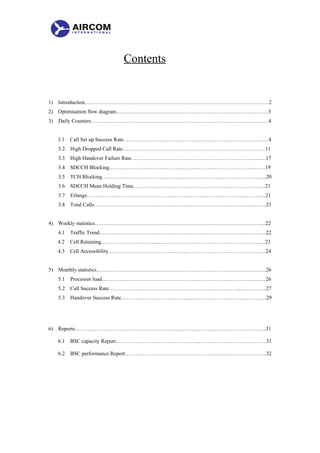
28. The call set up trend clearly indicates the call set up problem in cell site 20 B .The possible reason
could be interference or traffic channel congestion. The trend shows that traffic channel congestion is
also playing the major role for traffic channel set up failure.
5. Monthly Counters
a-) Processor load (Per BSC basis)
b-) Call success rate ( per BSC basis)
c-) Handover Success Rate( per BSC basis )
5.1 Processor Load
This provides a useful means of investigating processor load trends and providing a warning when
processor load tends to maximum. More processors should be added to the network switches thus
avoiding overload. A comparison of Processor load is shown. Processor load statistic is pegged for
every hour.
FIG 17. (Processor Load of BSC CMSC1)

29. FIG 18. (Processor Load of BSC CBSC3)
5.2 Call Success Rate
Call success rate on monthly basis can reflect the overall network health and display the results of the
optimisation procedure taken to improve the network quality. Routine Procedures are defined to
conduct the necessary actions after monitoring daily and weekly basis counters. Monthly counters
describe that how effective the routine procedures are to optimise the network. Within optima Call
success rate can be monitored on BSC basis. The following figure shows deterioration in call set up of
BSC “ CBSC3 ” specifically on 6th
, 14th
and 16th
November. “ APZ ” window within optima can show
CSR graphically. ( fig 19 )

30. FIG19. ( call set up analysis )
More generalised display can be possible by focussing on the particular cells which have higher drop
calls Using Custom queries. Specific BSC can be filtered and defining the thresholds in“ parameter tab
”allow the user to sort out the problematic cells. As the screen shows ( fig 20) BSC “ CB2 ” has higher
call drops between 24th
and 26th
of November.The Graph shows the accumulative no of call drops for
each hour taking into consideration the all cell sites within that BSC.

31. FIG 20. (call drop analysis )
5.3 Handover Success Rate
Handover success rate on monthly basis will show the overall “ Hand off ” behaviour of the network.
Within optima window, the handover window shows cell to cell handover data in statistical tables,
graphs and histograms. You can analyse the network over a period of time that you define and can
easily find and monitor badly performing handovers. Handover drops have been shown for one of the
cell sites and its neighbour for one month. HOCNT can also be monitored to check if the neighbours
are defined accurately. In normal routines HSR should be observed on BSC basis for monthly statistic.

33. 6. Custom queries /Reports
There are number of reports that can be generated from “ custom query “ windows of optima
on BSC and cell basis. Taking into account the BSC performance following reports are helpful
in analysing network quality.
a-) BSC capacity/traffic Report
b-) BSC performance Report
6.1 BSC CAPACITY REPORT
Within BSC all those “cells “ can be sorted out which are either carrying traffic “ too low “ or “
too high “. If the site is carrying large amount of traffic “ load sharing “ sites should be planned
to cater increased amount of traffic. For the case where traffic is too low other performance
counters like call set-up rate, dropped call rate and interference should be monitored. The tool
provides the option to generate these reports in “ EXCEL “. DTCH (dedicated traffic channel)
and TCH (Available no of traffic channel) indicate the capacity on cell basis and are shown on
optima screen.
Fig 21 ( BSC capacity report )

34. Fig 22 (BSC capacity report in excel format )
6.2 BSC PERFORMANCE REPORT
BSC performance report will point out all those cells with RF issues. Keeping in mind the
basic thresholds specified earlier, a BSC performance report should display total call drops,

35. call drops at bad signal strength and call drops at bad quality, Call congestion, Handover
success rate etc ( fig 23 )
Fig 23 ( BSC performance report )

36. The tool represent the measurement on per hour basis for every day taking into account all
the cell sites within the same BSC. The best method to observe BSC counters is to define
them on “ busy hour averages “ and they should represent the performance of the BSC as a
whole.