Wellbore hydraulics

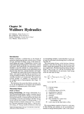
Chapter 34
Wellbore Hydraulics
A.F. Bertuzzi, Phillips Petroleum Co.*
M.J. Fetkovich, Phillips Petroleum Co.
Fred H. Poettmann, Colorado School of Mines*
L.K. Thomas, Philhps Petroleum Co.
Introduction
Wellbore hydraulics is defined here as the branch of
production engineering that deals with the motion of fluids
(oil, gas, and water) in tubing, casing, or the annulus be-
tween tubing and casing. Consideration is given to the
relationship among fluid properties, fluid motion, and the
well system. More specifically, the material presented is
intended to describe methods for solving problems as-
sociated with the determination of the relationship among
pressure drop, fluid rates, and pipe diameters and length.
To maintain the scope of this section within prescribed
limits, some material and data that are pertinent to the
solving of wellbore problems. but which can be found con-
veniently elsewhere, are not presented. The material not
covered includes (1) methods of measurement and
(2) complete data on fluid properties (See Chaps. 13,
16-19, 24).
The theoretical discussion that follows provides a ba-
sis for the development of correlations and calculation
procedures in subsequent parts of the section.
Theoretical Basis
Fluids in Motion
Energy Relationships. The energy relationships for a
fluid flowing through tubing, casing, or annulus may be
obtained by an energy balance. Energy is carried with the
flowing fluid and also is transferred from the fluid to the
surroundings or from the surroundings to the fluid. Energy
carried with the fluid includes (1) internal energy. U, (2)
energy of motion or kinetic energy (mv’/2g,.), (3) ener-
gy of position (potential energy m,gZ/g,.), and (4) pres-
sure energy, pV. Energy transferred between a fluid and
‘Authors of the orlgmal chapter on !hls fop~c I” the 1962 edmon Included these
authors and J K Welchon (deceased)
its surroundings includes (1) heat absorbed or given up,
Q, and (2) work done by the flowing fluid or on the flow-
ing fluid, W.
The conservation of mass, or the first law of thermo-
dynamics, states that the change in internal energy plus
kinetic energy plus potential energy plus pressure ener-
gy is equal to zero. The following energy balance between
points 1 and 2 in Fig. 34.1 and the surroundings illus-
trates the relationship for the previously listed energy
terms for unit mass of fluid.
2 2
U,+~t~z2+P2Vz=U,+1’1+~z,
%c g, Q,. g,
+p,V,+Q-W, . . . . . . . . . . . . . . . . (1)
where
U = internal energy,
v = velocity,
g,. = conversion factor of 32.174,
g = acceleration of gravity,
Z = difference in elevation,
p = pressure,
V = specific volume,
Q = heat absorbed by system from
surroundings, and
W = work done by the fluid while in flow.
This energy-balance equation is based on a unit mass
of fluid flowing and assumes no net accumulation of
material or energy between points 1 and 2 in the system.

34-2 PETROLEUM ENGINEERING HANDBOOK
Point 2
Point 1
Fig. 34.1-Illustration of energy-balance relationship.
Eq. 1 also can be put in the form
au+~+Lz+a(pv)=Q-w. . . . . .
c gc
since
Sl VI
and
s
s2
TdS=Q+Ef
Sl
where
T = temperature,
S = entropy, and
EP = irreversible energy losses, and
VI Pl
Eq. 2 can be put in the more familiar form
s
P2
2
v@+K+&=-W-E~. _. .
Pl
%c gc (3)
Since, in the system shown in Fig. 34.1, there is no work
done by or on the flowing fluid, W is equal to zero and
the following equation results.
-Et. . . . . . . . . .
If flow is isothermal and the fluid is incompressible, Eq.
4 may be simplified to
2 ; Nv2) ; &&7=-E
%c gc
p, .
P
(5)
where p =density .
The dimensions of the energy terms in Eq. -5 are ener-
gy per unit mass of fluid, such as foot-pounds per pound.
Quite often the force term is canceled (incorrectly) with
that of the mass term resulting in the dimensions of length
as of a column of fluid. For this reason, these terms fre-
quently are referred to as “head,” such as feet of the fluid.
For most practical cases, the ratio g/g, is essentially
unity. Although the terms in Eq. 5 are sometimes ex-
pressed as feet of fluid, no serious error is involved. In
fact, one can derive a very similar expression where the
terms are expressed in feet of “head.”
Eqs. 4 and 5 are the energy relationships that provide
the basis for the computational methods of the sections
to follow.
Irreversibility Losses. The use of Eqs. 4 and 5 requires
a knowledge of Et, the term that accounts for irreversi-
bilities (such as friction) in the system. The term E, can
be expressed as follows ’:
fiftv2
Et=- 2g,d, . . . . . . . . . . . . . . . . . . . . . . . . . . . . . (6)
where f commonly is referred to as a friction factor, L
is length, and d is pipe diameter. The friction factor, f,
usually is expressed in terms of the physical variables of
the system by correlations of experimental data.
For single-phase flow, the dimensionless friction fac-
tor, f, has been correlated in terms of the dimensionless
Reynolds number dvp/p with p being viscosity. A rela-
tionship is also suggested by application of dimensional
analysis to the variables involved. In either case the result
is
f=FIE, . . . . . . . . . . . . . . . . . . . . . . . . . . . ...(7)
CL
where F1 is a function of Reynolds number.
Eq. 7 has been the basis for correlation of considera-
ble experimental data for single-phase flow over the past
years. Eqs. 5, 6, and 7 have been adapted to multiphase
flow. Consideration of the character of pipe surfaces as
absolute roughness, E (that is, the distance from peaks to
valleys in pipe-wall irregularities), which may be ex-
pressed as a dimensionless relative roughness factor, t/d,
has led to improvements in correlations of single-phase
flow experimental data
f=F2[(3 (3, (8)
where F2 is a function of Reynolds number and relative
roughness.

WE lLLBORE HYDRAULICS
0.1
009
aQ8
007 0.05
0.04
3“, NJO.06 0.03
8 ‘005
0015J ;;;
004 0.01E s
G 0.03
$382 g
?
___-
F ^^^_l/llI I llllli
0.004 i
r-r
34-3
u- UUL36 0.002 i
5 002 %%s E
E o.aX% 5
0.015
cl0004 ;
oooo2
0.ooo1
001 &j&r
fTMnAK
=0.000,005 j”-‘“ti
00090.008 QooO,Ol
lb3 2 3456Bl14 2 3456B15 2 345681s 2 345681, 2 345681
IO IO A,, IO lo8
REYNOLDS NUMBER Re = =
P
Fig. 34.2-Friction factor as a function of Reynolds number with relative roughness as a parameter.
Fig. 34.2 shows the correlation for single-phase flow
according to Eq. 8. * Similar plots are found in the liter-
ature in which other friction factors are plotted as a func-
tion of Reynolds number. Care must be taken to avoid
confusion, as the same name and symbol are used for var-
ious multiples off as plotted in Fig. 34.2
The laminar-flow region, which extends up to a Rey-
nolds number of 2,000, is represented by a straight-line
relationship f=44/NR, on Fig. 34.2. Between 2,000 and
4,000, flow isunstable. Above 4,000, turbulence prevails
and the influence bf the physical properties decreases as
the Reynolds number increases. In fact, it is shown that
at very high Reynolds numbers the friction factor depends
solely on the relative roughness factor c/d.
since v2/2g, and El are equal to zero. Since g/g, is as-
sumed to be unity,
s
p2dp
-+Az=o. . . . . . . . . . . . . . . . . . . . . . . . ...(n)
PI
P
For the case of a static-liquid column, it is usually satis-
factory to use an average density for the column of li-
quid. Eq. 11 then can be expressed in the more convenient
and familiar form as
Ap=pAz. . . . . . . . I.. . . . . . . . . . (12)
The preceding theoretical discussion concerning irrever-
sibility losses is based on considerations involving single-
phase flow. Nevertheless, the material presented will pro-
vide a basis for considerations involving both single- and
multiphase flow that appear in the following seCtions.
The preceding equations will provide a basis for the cal-
culation procedures of the following sections for static-
fluid columns.
Static Fluids
Many wellbore problems are associated with static-fluid
columns, either oil, water, or gas, or combinations there-
of. In the case of static-fluid columns, Eq. 4 is applicable
in general and reduces to
s
P2
vdp+Qz=o . . . . . . . . . . . . . . . . . . . . . . .
PI
gc
or
p2dp
s-+542=0,. . .... . . . .
PIP gc
Producing Wells
Gas Wells
Calculation of Static Bottomhole Pressures (BHP’s).
Static BHP’s are used to determine the deliverability of
gas wells (backpressure curve) and to develop reservoir
information for predicting reservoir performance and
deliverability. Several methods for calculating static
BHP’s have appeared in the literature.3-6 The methods
differ primarily as a result of the assumptions made. All
start with Eq. 9 assuming g/g, is unity for a static
column:

GAS GRAVITY (AIR=0
Fig. 34.3-Pseudocritical properties of condensate well fluids
and miscellaneous natural gases.
If the column is vertical, aZ=L, where L is the length
of the pipe string, and Eq. 9 can be put in the form
s
PI
l’dp=L. . . . . . . . . . . . . . . . . . . . . . . . . . . . ..(13)
P2
If the column is not vertical, but inclined with the verti-
cal by an angle 8,
U=L c0se
and again usiq L, Eq. 9 becomes
s
PI
Vdp=L sins. . . . . . . . .(14)
P2
Subsequently, only the vertical column will be considered
and Eq. 13 will be used. Since
v=E. ...............................(1%
MP
where
z = compressibility factor,
R = gas constant, and
M = molecular weight,
Eq. 13, upon pbstitution, becomes
. . . . . . . . . . . . . . . . . . . . . . . . . (16)
For a particular gas, RIM, which is equal to 53.2411~~
where 7X is the gas gravity (air= 1.O), is a constant.
Therefore, Eq. 16 can be simplified to
53.241 PI
s
zT*=L. . . . . . . . . . . . (17)
YR pz P
It is at this point where certain assumptions are made and
calculation procedures differ. Assumptions are made in
regard to z and T.
For any calculation procedure, four “surface” proper-
ties must be known: well-effluent composition, well depth,
wellhead presske, and well temperature. The gas com-
position is used to calculate the pseudocritical properties
ppC and TPCof the gas, from which is estimated the value
of the compressibility factor z used in the calculations.
Quite often, gas composition is not available and gas
gravity must be used to estimate the pseudocritical prop-
erties (Fig. 34.3).4
A recommended method assumes constant and average
temperature T and allows z to vary with pressure. With
temperature being constant, Eq. 17 becomes
53.241?
s
PI z
-dp=L. . . . . (18)
YR P2 p
The method using Eq. 18 was suggested by Fowler.’
Poettmann4 made the solution of Eq. 18 practical by
presenting tables of the function
s
PPr z
0.2
in terms of ppr and Tpr. The tables are presented here
as Table 34.1.
It can be shown that
sp’fdl’=s (p,r), z--dp,, = fppr’’kdppr
Pi7 (P,,)? Ppr 0.2 PPr
(PPJ > z
-
s
-dppr. . . . . . . . . . .
0.2 PPr
(19)
An advantage of this method is that it is a direct method
of calculating >BHP. No trial and error is involved. In
terms of ppr and T,, Eq. 18 becomes
53.241?
L=-
YR [s
(P,,), z
0.2
p,,dp,r - I( ‘““’ &dppr]
0.2
(20)
By rearranging,
I
(p,,), 2 L-y, + (PP’)> z
-dppr = F
PPr
s53.241T o,2
_ dppr.
0.2 PPT
. . . . . . . . . . . . . . . . . . . . . . . (21)
Eq. 21 permits a direct solution for the static BHP.

WELLBORE HYDRAULICS 34-5
Pseud+
reduced
PWSSUrE
PO,
i:
i:
i!
08
Yo’
1:
I 3
I:
I 6
I 7
I!
20
::
::
2s
:;
5:
::
::
35
TABLE 34.1-VALUES OF S‘PP’Ldq,,
0.2 PPI
Pseudoreduced Temperature. lpr Pseudo Pseudoreduced Temperature, Tpr
reduced
Plf%SUR
I 05 I I IO I I5 I 20 I 25 I 30 I 35
pm
I 40 I 45 I 50 I 60 I 70 I 80 I 90
0 IO 0 0 0 n 0
0 350 0 350 0 35C 0 350 0 350 0 3jU 0 3X)
0 615 0 619 0 623 0 626 0 625 0 63U 0 632
0 805 0 816 0 826 0 834 0 83'1 0 844 0 848
i: 00 350 00 350 00 350 IO0 350 [O0 350 00 350 100 3%
:: ,fl0 033851 00 634 0 63j 0 636 0
854,O 856,O 860,O
637862 00 638864 00 86b639
0 955; 0 971 0 985 0 YQl3 I 01 I I 022 I 032’ 0 6
I 078 I IO0 I I24 I 145 I I62 I 178 0 7
I I75 1 207 I 23Y I 264 I 285 I 300
I 190,
I 3131 0 8
I 256, I 3W I 335 I 365 I 3Rb I 403 I 417, 0 9
I32711 375’1 420 I455 I47Y I 500 I415 IO
1: I 682 I 6% I 710 I 737,l 75) I 761 I 770
I 3 I 746 I 758 I 77’) I 810 I 828 I 836l I 845
1: II 810867 ! II 825884 II 8479-36 II 882, IIY3U, 903962 ~II 911973 ’1 II 920984
3801 I 438 I 435 I 528 I 552 I 573 I 591
433 I 500, I 550 I hO0 I 625 I 645 I 666
4b3: I 545 I 602 I 657 I 684 I 709 I 731
492’ I 590 I 654 I 713 I 742 I 772 I 7Y5
510 I 620, I 6W i I 757 I 7YI I ~24 I 848
527 I 649, I 7Zh I 800 I 819 I RI5 I 9C”l
544: I 670’ I 754 I 834 I 876 I ‘117 I 443 ~
560, I hW/ I 782 I 867 I VI> I 9>H I ‘It35
575 I I 708, I 808 I KY6 I Y44 I 991 2 ULZ
590 1 I 725 I 833, I 924 I 975 2 027 2 05Y
, b I 923 I 943 I 964 I 913 2 021 2 035l 2 047’
I 7 I 96Y I WI 2 012 2
I a 2 014 2 038 2 060 2
043’2 072 2 089~ 2 IO2
093’ 2 I23 2 142 2 157
:; ‘2OY32 054 22 079 2 IW 2
I 1 i
604 I 743, I 854~ I 947 2 00) 2 057 2 UC12
6171 I 761 I 876’ I 971 2 031 2 086 2 I25
631 i 1779’1 RY7; IVY4 2 059 2 II6 2 I57
644 I 7971 I 919 2 018 2 087 2 I45 2 IW,
658: ,815, I 9M 2 041 2 II5 2 I75 2 223
6721 I 830 I 95R 2 061 2 137 2 I98 2 2491
685 1 845’ I 976 2 081 2 159 1221 2 275 ~
699, I MO I 994 2 IO1 2 180 2 245 2 1021
712ll875’2012,2i2I 2202 12bH 23281
726 I 690, 2 030 2 140 2 224 1 LYI 2 354’
,22 12b12I60 2
II912 140~2
136178’22072 165’2 223Il225U187, 2 204
:: 1RL2I53 2 212176 22 215’2252 2 2R8248 22 272lL513’2 192334
2 3 2 IY3 2 222 2 249 2 288 2 329 2 354 2 375
2 4 2 22712 256’2 285 2 325 2 3b9 2 395 2 417
2 5 2 260 2 2% 2 521 2 362, 2 410 :2 436 2 459
2 6 2 206 2 318 ’2 350 2 392 ’ 2 442 ~2 069 ~2 492
2 7 , 2 316, 2 347 2 379 2 423 / 2 474 2 502, 2 525
2 8 2 344, 2 375 (2 407 2 413 2 506 2 534 ~2 ii7
2 9 I 2 372 j 2 404 i 2 436 2 484 : 2 538 2 567 2 5W
3 0 12 Q33 I 2 432 ,2 465 2 514 2 570 ,2 600, 2 623
740 I ‘XI4 2 046 2 157 2 243 2 >II 2 376
754 I 918 2062 2 175 2 261 2 >?I 2 397;
767 ,Y3212O78 2 l92;2 280 2 350 2 419
781!1946i2094 2210 2298 1370 2440:
795 I 9tQ 2 I10 2 227 2 317 2 3’10 2 462
!IBo8 1974’2121 2243’2333 24fl7 248Oi 3 6
2 4Y8
: 2 535’ 2 568 ’ 2 603, 2 664 2 726 1 7hb 2 7Y2
I 622 I 988 2 14U 1 ii9 2 34’) 1 424 3 7
2 275’2 365
,2 556 2 5138 2 624 2 686 2 748 1791 2 RI7
I 835 2 GO2 2 I55 2 4411 2 5171 38 ;2576:2 bOY 2644'2708 2771 181j 2843
:i II 049R62 22 Olh030 22 166170 12’112 306 22 381397 22 457474 22 5351533
:: II 875889’ 22 044058 22 201216 12 111336’2 2 413429 21 4Y0506 22 56’9586’
4 3 I I 902 2 073 2 2311 2 351 2 444 2 523 2 602
44
45
, I 916 2 OR7 2 245 2 )06 1 460 2 ij9 2 619
I 919 2 101 2 260 2 381 2 476 2 555 1 635
46 1942 2115 2274 2195 24YI 2570 2651 4 6 ~2 719 2 754 2 793’2 863 2 933 2 9W 3 022
47 I 955 2 I28 2 238 2 009, 2 507 2 506 2 6b6 4 7 ~2 735 2 770 ’2 810’ 2 881 , 2 952 3 DO9 3 041
48 I Y6V 2 142 2 301 2 423 2 522 2 601 2 682 4 8 2 752, 2 786 ~1 I326 I2 899 2 970 3 027 3 061
4 9 / I982 2 I55 2 315 2 437 2 5% 2 617 2 697 4 Y 3 046 3 080
50 I 995 2 169’ 2 329 2 451 2 553, 2 632 ~2 713 5 0
2 768 2 802 2 043 2 917, 2 989
2 784 2 RI8 ~2 WI, 2 935 3 007 3 065 3 IM)
: : I22 009’024 22 I83197 22 342355 22 465479l 22 567581 22 046hbl
2 4Y2’ 2 5%
22 728743 552 I ~22814799 22850’2892834 ~2 876 / 22968’3042952’ 3 024 33OY9082 33 136I I8
5 3 2 038 2 210 2 369 2 675 2 758
5 4
~
2 053 2 224 2 382 2 506 2 609 2 bW 2 773
5 5 2 067 2 238 2 395 2 520 2 623 2 704 2 78A
F; ~22 07’)O’JI 22 251LO4 22 408421 22 533547 16361 hiU 22 718731 22 MIRI5
:; 22 102II4 22 277210 22 435440 22 560574 22 663677 2L 74i75H 22 R42RZR
60 2 I2h 1303 2 461 2 587 2 O’K) 2 772 2 855

’96
i i
2585.2755I2908’3034 3 I31 3216 3302 i! 3 376 3 424 ’3 475 3 585 3 644 3 713 3 7M)
12 622 12 702 2 942 3 068 ~3 164 133 251 3 33A 9 9 3 41 I 3 458 3 510 3 599 3 679’
2/ 2 610597’2 2 767780 ~22 919a931 133 045,3057 3 14283I53 228239 33 314326 9 8 33 39Y1HR 33 435,447, 33 467495 33 576,508, 33 6%bb7 )i 1 33 724736 33 772783
9 9 , 3 747 3 795
IO 0 2 634 2 804 2 954, 3 080 3 175 13 263 3 350, IO0 ‘3423,3470,3521~3610 3691
~
3758 3806
IO I 2 646 2 816’2 966’3 092 3 I87 I 3 274 3 361 IO1 13434 3482:3532 3622 3702
IO 2 2 658 2 828 2 97R 3 103 3 199 3 286’ 3 372, IO 2 ’ 1 446 3 494 3 544 3 633 3 714
3769 3817
3 780’3 628
I03 3 790 ‘3 840
IO 4
i2671 2840 2989 3115 3211;3297,3382~ I03 3 457 3 506 3 555 3 h45 3 725
105
; 2 683 2 852, 3 001 3 I26 3 223 ’3 309 3 393 I; ; 3 464 3 518, 3 5b7 3 656 3 737
2 695’ 2 864 3 013, 3 I38 3 235 13 320 13 404 3480 3530 3578 3669 3748
3 801 [ 3 851
3812 3862
IO b 2 707 2 876 ~3 025 3 I50 3 246 ’3 332 1 3 416 IO 6 3 492 i 3 541 3 588 i 3 679 3 758
! 2 719 2 888 ! 3 037, 3 I61 3 258 I 3 343, 3 428 IO 7 3 504 3 552, 3 598 3 689 3 769
3 823 3 073
IO 7
‘2 732 2 900’3 048’3 l73l 3 269;3 355 3 440 IO 8 3 51513 56213 60913 700 3 779
3 834 3 883
IO 8
II 0
(2744 2912 3060~31R4~3281t3366 3452 IO 9 3 527 3 573 3 619 ; 3 710 3 790
3 844 3 894
109
/
I I I
2 756 2 924 13 072, 3 1% 3 292 3 378, 3 464 II 0 3 539 3 584 I 3 629 3 721 13 BOO
3 855 3 904
3 866 3 915
II I
II 2
II 3
II 4
II 5
II 6
II 7
II 8
II 9
I2 0
2 768 2 936 I3 084 3 208 3 304 3 389 / 3 475 3 551 3 595 3 639 3 732 ~3 81 I 3 877 3 926
2780 294R:3096 3220,3315 34UIl3486 3562’3605’3650’3743’3822 3888 3937
2 793 2 960’ 3 I08 3 231 / 3 327 3 412 3 497 3 574 3 616 3 660. 3 753 3 832 3 899 3 947
2 805 2 972, 3 129 3 243 3 338 3 424 3 508, 3 585 3 626 3 671 3 764 3 843 3 910 3 958
2 817 2 984l3 132’ 3 255 3 350 3 435 3 519 II 5 3 5Y7 / 3 637 1 3.631 ’3 775 3 854 3 Y2I / 3 969
2 829 2 996 3 144 3 267’ 3 361 3 446 3 529 II 6 3 607 3 648, 3 692 3 756 3 865 3 932 3 980
2 841 3 008 3 156 3 279 3 373 3 456 3 543 II 7 3 617 3 65A 3 702 3 797 3 R7h 3 943 3 991
2 854 3 020 3 I68 3 290 3 384 3 467 3 550 II R 3 h!9 3 660 3 713 3 808 3 886 3 95514 W3
2 866 3 032 3 It33 3 302 3 396 3 477 3 561 II 9 3 h14 3 b79 3 723 3 819 3 R97
2878 3044,3I92 3314,3407,3488 3571 I2 0 3 h48 3 bW 3 734 3 830 3 908
3 966, 4 014
3,977, 4 025
TABLE 34.1 -VALUES OF s
p, 2
-dpp, (continued)
0.2 PPI
PSWd3
reduced
Pseudoreduced Temperalure, Tpr Pseudo-,
reduced
Pseudoreduced Temperature, T,,
PlfJSSUre
’ ’ P~0SS”E ’PO, I 05 I IO I I5 I 20 I 25 I 30 I 35 p!x I I 40 I 45 I 50 I 60 I 70 I I 80 I 90
~~ _~ ---I
,
-/-
61 2 139 2316 2 474 2600 2703’2 785 2 869 6 I 2 943 2 984 3 029 3 II I 3 I87 3 250 3 292
62 2l52~2328 2486 2bl2 2716 2799 2882 bl 2 956 2 997 3 043 3 I25 3 LO2
2 16512 341 2 499 2 025 2 729 2 Ml1 2 896 6 3 1 IWO 3 OII 3 056 3 I40 3 218
3 266 3 308
3 281 3 323
2 YHl 3 024 3 070 3 I54 3 233 3 297 3 339

TABLE 34.1-VALUES OF ippLdp,, (continued)
0.2 PPI
’ Pseudo-
I reduced
Pressure
PP
::
6J
64
65
66
67
68
4:
7 I
72
::
75
’ z:
83
84
RI
86
~ 07
88
:z ~
9 I
;:
2:
/
96
97 I
98
99
Pseudoreduced Temperature. T,Pseudo PSBudOreduCed
reduced
Pressure
PP I 2ccl 220 ,240
__~.
02 0 0 0
0 3 ’ 0 350 0 150 0 J50
ii: 00867639 00868640 00 640869
i; II 050216 lI 0512lR II llil219
it II 489360 II 492%J II 4945114
1.0 , 602 1 I 607 I 608
I:; i II 691780 / II 699790 II 702795
13 I 851 1 I 868 I 875
I? / I, 915997 ~ 2I 945010 I 2I 954019
260 z&300
rempmure. rp
260 280
---I ~~~
: 150 ; Ji”
0 640 0 CT40
0 8b9 0 869
2 074 , 2 083
2 III I 2 141
; y; I
2;5 I
: ;“4;
2 2 29%
2 326 / 2 J37
2 366 2 JR0
2 407 / 2 422
2 447 2 465
2 488 2 507
2 523 / 2 544
2 559 2 MI
2 594 2 617
2 630 2 654
2 665 / 2 691
I
2 670 ~ 2 694 2 722
2 700 2 723
1
753
2 729
2
2 J52 2 783
J4 2 759 2 78) 2 814
35 2 788 2 810 2 845
:; 2 813 1 2 836 2 a72
; .s% ; g; 2 899
:.G! 2 925
2 890 2 914 2 952
4.0 2 915 ~ 2 940 2 979!
I 052 I 052
I 220 I 220
I Jf 4 ~ I J64
I 4Oj 1 I 495
I WI9 I 611)
I 706 ~ I JUY
I 802 I hU8
I 1)MJ I 2490
I 964
1
I
I )7?
2 027 2 UJ6
2 090 2 100
2 I48 i 2 1%
2 205 2 217
2 256 2 267
2 347 ~2 317
2 350 ’ 2 ibl
2 394 2 404
2 4JJ 2 448
2 481 2 491
2 524 2 5Ji
2 562 2 574
2 599 2 012
2 bJ7 2 051
2 674 2 6k9
2 712 2 728
2 744 2 7%
2 775 2 JW
2807 2821
2 BJM 2 H52
2 a70 2 883
2 910 2 911
2 950 2 YJB
2 990 2 966
J OJO 2 99J
J 070 i 3 021
loo 2 20 2 40Jo0
: J50
0 640
0 at9
3 321 3 362
3 JJJ J 379
3 154 J 395
3370 3412
3 387 3 429
3 402 3 444
3 417 3 459
3 432 3 475
J 447 3 490
1 462 3 505
3 477 3 520
3 491 I 3 534
3 506 1 3 549
3 520 J 563
3 535 3 578
3 548 J 591
3 562 3 605
3 575 3 618
3 5R9 3 bJ2
J 602 3 645
3 615 J 658
3627 3671
1 640 3 684
3 652 3 fJQ7
3 665 3 710
3 677 3 722
3 690 3 714
J 702 J 746
J 715 3 758
3 727 ’ 1 770
3 719 3 782
3 7% / 3 794
3 762 3 X06
3 77J J RIB
3 785 I 3 830
3 797 J 042
J R(r) J 854
3 820 J 865
7 RJZ J R77
3 4U9
J 426
3 44J
3 460
J 477
3 493
J 508
J 524
3 539
3 555
3 570
3 584
3 599
3 613
3 628
3 642
1 656
3 670
J 684
3 690
J 442 J 466 J 4i7
1 4j9 J 483 J 494
3 4?6 J 501 J 511
J 49J , 518 3 526
3 510 3 536 J 54;
3 526 3 551 J 561
3 542 3 507 J 577
3 557 3 582 J 592
3 573 3 598 3 608
3 5139 3 613 3 624
I ii:I Jh4
I 49)
I 6,”
I 711
I RI2
I 89b
I YHU
2 045
3 628 3 6J9
3 643 3 654
6659 3670
3 674 3 685
3 689 3 700
3 703 3 714
3 718 1728
3 JJ2 3 742
3 747 3 756
3 761 3 770
3 774 J JRJ
3 788 J 796
3 801 J 810
3 815 J 82J
3 R18 J 836
3 840 3 a49
3 853 3 862
3 865 J 875
3 878 : J 888
3 890 , J 901
3 902 / 3 91)
3 915
3 927
3 940
/
3 925
3 9J8
3 950
3 952 J 962
3 964 J 974
3 976 J 980
3 987 J 999
3 999 4 01 I
4 OII 4 U2J
4 02J 4 OJS
4 035 4 046
4 046 4 058
4 ow 4 069
4070 40.31
4 081 4 092
4 093 4 IO4
4 104 4 II5
4 116 4 127
4 127 4 1%
5 604
3 618
3 633
3 647
3 662
3 676
1 33 690
(
704
3 718
/ 3 732
~3 745
3 758
3 771
3 784
3 797
3 810
3 a23
3 835
3 848
3 Ml
~3 873
1 3 885
3 897
~ 3 999
3 921
3 93J
3 94;
3 957
3 969
3 981
3 992
4 004
4 015
4 027
4 038
4 049
4 060
4 071
4 082
4 093
1.6 2 059
1.7 2 116
I.8 2 172
1.9 2 219
2.0 2 265
2.1
::
2.4
25
2.307
2 349
2 391
2 433
2 475
:;
:;
30
3.1
::
2 508
2 541
2 575
2 608
2 641
2 11”
2 lb9
2 227
2 279
2 3M
2 375
2 42U
2 4b5
2 itu
2 555
2 593
2 CiO
2 hbtl
2 JU5
2 743
2 775
2 806
2 8%
:tE
2 929
2 957
2 984
3 012
3 040
3 711
3 723
3 736
J 748
3 761
J 773
3 786
3 798
3 RII
3 823
: “8:s
3 859
3 871
3 481
3 R95
3 907
3 918
3 930
i 942
3 953
3 965
3 976
3 988
3 999
4.1
42
4.3
4.4
4.5
3 002
3 025
3 049
3 072
3 095
:;
48
49
5.0
; ;; ~
2 983 ~
: ;;
3 008
3.aJ5 3 010
3 028 3 053,
3 048 3.074
306a
JO881
3095
3 108 i
3 II5
3 136
3 128, 3 157
3 II? 3 147
3 119 J I68
3 161 3 190
3 18J 3 211
3 205 3 23)
3 081
JO92
1 IOJ
3 I14
J I25
IO 0 i 844
3 1145 3 064
3 iUb9 3 OR8 IO I 3 855
J lN4 3 112 IO 2 3 867
J118 1136 IO J 3 RJR
J 142 3 160 In 4 J A90
In.5 J 901
3164 3182
3 IPI, 1 zn3 ICI 6 3 912
3 2W 3 22i 10 7 J 92J
3 231 3 246 In a 3 9J3
3 253 3 268 10 9 3 944
II 0 3 955
3 274 3 2HX
3 295 3 JUH II I 3 ‘,f,6
:::I , 3J2xJ J4H IIII 2J 31 9779H”
3 ii? 3 JbB II 4 3 9’)9
II 5 4 0,”
3 175 3 JR6
3 39, I 4115 II b 4 1022
J 412 J 42J II 7 4 OJ4
1411, 1442 II a 4 04;
3 448 3 440 II 9 4 057
12.0I 4 069
3 689
1 900
3 911
3 923
3 934
3 945
J 956 4 010
J 9hJ 4 021
3 978 4 UJI
3 989 4 042
4 000 4 053
3 146 1 3 I??
1 lh4 3 IOil
5. I
52
::
55
56 3 235
i ili
3 2J5
3 255
3 273 321 3 352
3 291 319 3 JJO
3 309 356 J 389
3 127 374 3 407
3 345 392 3 425
3 225 3 253
3 244 J 27)
J 264 3 294
3 283 I J JI4
3 303 1 3 3J4
4 011
4 022
4 033
4 044
4 055
4 0117
4 IO4 4118 4149
4 I!6 4150 4IMI
4 127 4 101 4 172
4 I39 4 17) 4 IRJ
4 I50 4 184 4 1’14
4 I61 4 I95 1 4 20,
4 172 4 206 4 2lh
4 IRJ * 217 4 227
4 194 4228 42Jir
4 205 4 2J9 4 249
4 Ob4
4 075
4 1187
4 098
4 109
4 121
4 132
-

34-a PETROLEUM ENGINEERING HANDBOOK
Example Problem 1.4 Calculate the static BHP of a gas
well having a depth of 5,790 ft; the gas gravity is 0.60,
and the pressure at the wellhead is 2,300 psia. The aver-
age temperature of the flow string is 117°F.
From Fig. 34.3,
T,,<=358”R.
pQc =672 psia,
Tp,=i zz
117+460
Tp,
= 1.612, and
358
(Ppr) : =
2,300
___ =3.423
672
From Table 34.1.
s
(Ppr) _ 2
-dpP, =2.629
0.2 PV
and
LY, (5,790)(0.60) =o.l l3
53.241T = (53.241)(577) ’
Therefore, from Eq. 21
(p,J, 2
--dp,r =2.629+0.113=2.742.
From Table 34.1, 2.742 at a T,,r of 1.612 corresponds
to a ppr of 3.918. Then
p=3.918(672)=2,633 psia.
If temperature is linear with depth,
T=aL+b . . . . . . . . . . . . (22)
and
dT=a dL., . . .(23)
where a and b are constants. By substituting Eq. 23 in
Eq. 17 and putting in the differential form, the following
is obtained:
dT 53.2412 dp
-=-- . . . ..~.................
UT
(24)
YR p
Integrating,
53.241
I,n5=-
PI dp
Q T2
s
z-. . .
78 D, p
(25)
$) O1877yuLi(T:I = p[~0.01877~~0.744~~7.500)1/[~6125)(0.820)]
- 0.20x2
= 1.2239.
pi =(2,600)(1.2239)=3,182 calculated.
Since a=(T, -T7-)lL,
LI(T, -T2) L 53.241
=-=
In T,lT, TLM
s
PI dp
z--, . . (26)
-fg pz p
then
53.241Tm PI z
L=
s
. . . . .
78 P2
where
TLM=
TI -T2
In TIITz ’
(27)
T, and T2 are, respectively, bottomhole and wellhead
temperatures. It can be seen that Eq. 27 differs from Eq.
18 only in that here a log mean temperature TLMis used,
whereas Eq. 18 uses the arithmetic average temperature,
T.
Referring to the example as an illustration of the cal-
culation procedure using the log-mean-temperature con-
cept, TLM merely is substituted for 7’.
Another method of calculating static BHP in gas wells
is based on the following equation.
p,~p*e0.01877r,Ll~rz~ . . . . (28)
Eq. 28 can be derived from Eq. 17 if an arithmetic aver-
age temperature ? and an arithmetic average compressi-
bility factor Z are used. 7’he method using Eq. 28 is a
trial-and-error procedure. Values of p i are assumed to
obtain a value of Z. p t then is calculated. The procedure
is repeated until the values of p, are in agreement.
Example Problem 2. (Data used are from Ref. 5.) Given:
Well A
p2 = 2,600 psia,
78 = 0.744,
L = 7,500 ft,
T = 152.511~=612.51112,
PPC
= 663.8 psia (from Fig. 34.3), and
Tpc = 385.6”R (from Fig. 34.3).
First Trial. Assume:
p1 = 3,100 psia,
3 = 2,850 psia,
PPr = 2,850/663.8=4.30,
T,, = 612.51385.6=1.59, and
Z = 0.820.
Therefore,

Second Trial. Assume: and
pt = 3,182 psia,
p = 2,891 psia,
PP- = 2,891/663.8=4.36,
T,, = 1.59, and
t = 0.821.
Therefore,
p l = (2,600)(e0 2082),
= (2,600)( 1.2239)
= 3,182 psia calculated check.
Measured pressure at 7,500 ft equals 3,193 psia.
Calculation of Flowing BHP’s: Flow in Tubing. Flow-
ing BHP (BHFP) of a gas well when used with the known
static formation pressure provides the basis for evaluat-
ing the well’s deliverability. In wells that produce through
tubing and have no packer, the static column of gas in
the tubing-casing annulus is exposed to the producing for-
mation. In this case, BHFP. or sandface pressure, can be
determined by the relatively simple procedure of calculat-
ing the pressure at the bottom of the static column of gas
in the annular space. The preceding section describes this
calculation procedure. Where a gas well is equipped with
a tubing-casing packer. it becomes necessary to use the
flowing-gas column in calculating the BHFP.
Use of the flowing-gas column means that energy
changes resulting from frictional effects, as well as the
energy differences caused by the compressional effects
and potential-energy changes. enter into the calculations.
Several methods have been developed for calculating
the pressure drop in flowing-gas columns.‘.6.7 Sukkar
and Cornell’s method6 is described in detail. Raghaven
and Ramcy8 extended Sukkar and Cornell’s method to
cover reduced temperatures to 3.0 and reduced pressures
to 30. In a subsequent section that deals with gas flow
in injection wells, Poettmann’s’ method is described.
Poettmann’s method can be used for upward flow also.
The basic energy equation, Eq. 3, for any flowing fluid
in differential form is
vdr
l’d[>+-+%lZ-dEl-dW=O. .(29)
A,< SC,
Assuming that the kinetic-energy term is small and can
be taken as zero, and recognizing that dW, work done
by or on the fluid. is zero, Eq. 29 reduces to
Vdp+ %lZ+dEr=O. . . . (30)
g,
For vertical gas flow, dz=dL. Since
V=F ..... .... .... .... .... ..
WJ
(15)
K=l.O
g,
and
&y =fi2&
I 2g,d’ . . . . . . . . . . . . . . . . . .._........
Eq. 30, upon substitution, becomes
(31)
dL=O. . . . (32)
Velocity can be expressed in terms of volumetric flow
rate and pipe diameter. Pressure can be expressed in terms
of reduced pressure. Substituting these terms in Eq. 32,
integrating the equation, and converting to common units
results in
s(PP~’: (zlp,,)dp,,
-O.O1877y, j”‘F . (33)
(Ppr) ,
1 +B(z/p,,)2 =
Li
where
B=
667fq 2T2R
4’ppc2 ’
Y,q = gas gravity (air = 1.O),
L= length of flow string, ft,
T= temperature, “R,
T= average temperature, “R,
f= friction factor, dimensionless,
48 = flow rate, lo6 cu ft/D referred to 14.65
psia and 60”F,
di = inside diameter of pipe, in.,
Ppc = pseudocritical pressure, psia, and
Ppr = pseudoreduced pressure pip,,.
At this point, it is further assumed that temperature is
constant at some average value. This permits direct in-
tegration of the right side of Eq. 33, as
s(PP),(zbpr)dppr 0.01877
1+ B(zlp,,) 2
=-ygL,
T
. . .
(p,r) I
(34)
where the limits of the integral are inverted to change the
sign. If the temperature is linear with depth, the use of
log mean temperature as the average temperature provides
a rigorous solution to the right side of Eq. 34. This use
of log mean temperature confines the effect of the assump-
tion of constant temperature to the left side of the equa-
tion, where, for practical purposes, it is extremely small.
Thus, errors introduced by the assumption of constant
temperature are negligible.
(continued on Page 34-23)

TABLE 34.2-EXTENDED SUKKAR-CORNELL INTEGRAL FOR BHP CALCULATION
‘Pg.,W,,)dp,,
I
02
1 + WP,,?
Pseudoreduced temperature for B=O 0
Pp, 1.1 12 13 1.4 15 16 17 18 1.9 2.0 2.2 2.4 26 2.8 3.0
020 00000 00000 0.0000 0.0000 00000 0.000 0.000 0.000 0000 0.0000 0.0000 0 0 0.0000 o.oooo
0 50 08387 08582 0.8719 0.8824 0 8897 0.8966 0.9017 0.9079 0.9082 0.9108 0.9147 0.9177 09194 0.9206 09218
1.00 13774 14440 14836 15129 15334 1.5514 15654 15781 15623 15889 1.5986 1.6059 16111 1.6148 1.6184
1.50 1.6048 1 7373 1.8078 1.8565 1.8911 1.9192 1 9422 1 9609 1.9693 1.9798 19951 2.0063 2.0151 2.0211 2.0274
2.00 17149
2.50 17995
3.00 1.8750
3 50 1.9473
400 2.0178
4 50 20889
500 21547
550 22214
6.00 22872
19116 20157
2.0298 2.1631
21255 22778
20842 21331 2.1709 2.2023 2 2273 22397
2.2507 23138 23607 2.3996 24307 2.4469
2.3813 24570 2.5125 2.5583 2.5947 26148
2.4898 2 5762 2 6390 2.6909 2.7325 2.7561
2.5845 2 6793 2 7480 2.8052 2.8515 2.8784
2.6698 27715 2 8449 2.9065 2.9569 2.9867
2.7484 2 8558 29330 2.9982 3.0523 3.0645
2.8222 29341 30146 3.0828 31400 3.1742
28926 30079 30911 31616 32215 3.2575
22536
2.4641
26354
27798
2.9050
3.0158
3.1158
2.2744 2.2893 2.3013 2.3100 2.3184
2.4900 2.5081 2.5234 2.5347 2 5452
2.6654 2.6863 2.7050 2.7189 2.7314
2.8138 28382 2.6589 2.8752 2889622101 2 3746
2.2822 24603 2.9426 2.9699 2.9928 3.0114 3.0274
3.0571 30871 31119 3.1322 31496
3.1605 3.1930 3.2195 3.2413 32597
3.2552 3.2899 33178 3.3408 33600
3.3428 33795 34085 34325 34524
2.3622 2 5390
2.4330 26128
25013 26833
2 5577 27512
3.2074
3.2924
6.50 23522 2.6329 28171 29603 30781 31635 32360 32980 33355 3.3720 3.4245 34629 34931 35176 35381
7.00 24165 26971 28814 30258 31452 32324 33065 33704 3.4092 3.4470 3.5012 35411 35722 35973 36181
750 2.4802 27602 2.9442 30893 32100 32985 3 3740 34393 3.4792 3.5180 3.5738 36148 35467 36723 3fi934
8.00 25432 28223 30058 31512 32727 33623 34387 35052 35460 35857 3.6486 36847 3.7173 37432 3.7646
850 2.6057 28836 30664 32118 3.3338 34239 35012 35685 36101 36504 3.7144 37512 37844 38108 3.8323
29441 31260 3 2713 3.3934 3 4838 35617 36297 36718 3 7126 3.7775 3.8148 38484 3.8750 3.8969
30039 3.1847 33296 3.4516 3 5422 36204 36889 37315 3 7727 3.6382 3.8760 39099 3.9357 3.9588
30630 32427 33870 3.5087 3 5993 3 6776 3 7465 3 7894 3 8308 3.8969 3 9350 3.9690 3.9961 40182
31215 3.2999 34436 3 5647 3.6552 3 7336 3 8026 38456 36672 39538 39921 40262 4.0533 4 0755
31794 3.3565 34993 3 6198 3.7100 3 7883 3 8573 3.9004 3 9421 4 0090 4 0473 40814 4.1086 41309
32369 34126 35543 36741 3 7640 3.8420 39108 3.9540 39958 40627 4.1010 4.1351 4 1622 41845
32940 3.4681 36086 3 7277 3.8171 3 8948 3 9634 40065 40432 41150 41532 41872 42143 4 2366
33506 35231 36623 37806 38694 39467 40150 4.0579 4.0994 41660 42041 4 2380 4 2650 4 2872
34068 3 5777 3.7154 3 8328 3 9211 3 9977 4 0557 4.1084 4.1495 4 2158 42537 42875 43144 4.3365
34627 36319 3.7680 3 8644 39721 40480 4 1155 4 1580 4.1989 4 2845 43021 43357 43625 4.3846
35183 36857 88200 39354 40224 40977 4 1547 4 2067 4 2472 4 3122 4 3494 4.3829 4 4095 4.4316
35735 3 7391 38716 39859 40722 4 1400 4 2131 4 2546 4 2947 4 3589 43957 4 4289 44555 4.4775
36285 37922 39228 4.0349 41215 4 1950 42609 43018 43414 4.4047 4 4410 4 4741 4 5005 4 5224
1550 34335 36832 38450 39736 4.0855 4 1702 42428 43080 43483 4 3874 4.4497 4 4855 4 5183 4.5446 4 5663
16.00 34906 37376 38974 40240 41346 42185 42900 43546 43942 44327 4.4939 4.5291 45617 45878 46094
16.50 35474 37919 39497 40740 41833 42663 43388 44007 44395 44773 4.5374 4.5720 46042 46302 46518
1700 36041 38459 40016 41237 42316 43138 43830 44462 44843 45213 4.5802 4.6141 46461 46719 46933
1750 3.6606 38996 40533 41731 42795 43608 44289 44913 45285 45648 46223 4.6555 4.5872 47129 47341
1800 3 7170 39532 41048 42221 43271 4.4075 44743 45359 45722 46077 4 6638 4.6963 4.7276 4.7532 4 7743
1850 37732 40066 41560 42709 43744 44538 45193 45801 46154 46501 4.7048 4.7365 4.7675 4.7928 48138
1900 38293 40599 42071 43195 44214 44998 4.5640 46239 46582 46921 47451 4.7761 4.6067 46319 48527
900 26676
9.50 27289
1000 27896
10.50 2 8499
11.00 2 9096
1150 29690
1200 30280
1250 30867
1300 31452
1350 32033
1400 32612
1450 33189
1500 33763
1950 3.8853
2000 3.9411
20 50 3.9969
2100 40525
21 50 4.1080
2200 41634
22 50 4.2187
2300 4 2739
2350 4.3291
24.00 4.3841
24.50 4.4391
25.00 4.4940
2550 4.5488
2600 4.6036
41129 42579 43678
41658 43086 44158
42186 43590 44636
42712 4.4094 45112
43237 44595 45586
43760 45095 46058
44282 4 5594 4.6528
44803 4 6091 46996
45323 46587 4.7463
45842 47081 4.7928
4 6360 47575 48391
4.6877 48067 48853
4.7392 48558 49314
4.7907 49048 49772
4.8421 49536 50230
4.8934 5.0024 50686
4.9447 5.0511 51142
49958 5.0997 51595
50469 5.1462 52048
50979 5.1966 52500
51488 5.2450 52950
51997 5.2932 5.3400
4 4681 45455 4 6053 46574 47006 47335 4 7850
45145 4.5909 46522 47104 47425 4 7746 4.8244
45606 46360 4.6959 4.7531 4.7841 48152 48633
46065 4.6808 4.7392 4 7955 4.8253 4 8554 49017
46522 47254 4.7822 48376 4.8662 4 8953 4.9397
46976 4 7697 4.8250 48794 4.9068 4 9348 4.9774
4.7428 48138 4.8675 4.9209 4.9470 4.9739 5.0146
47879 48577 4.9098 49621 49869 50128 50514
48327 4.9014 4.9518 50031 5.0265 5.0513 50879
48773 49449 4.9935 5.0438 5.0659 5.0895 5 1241
49217 49882 5.0351 50843 5.1050 5.1275 5 1599
49660 50312 5.0764 51245 5.1438 5.1651 5.1955
5.0101 50741 51176 51646 5.1824 5.2025 5.2307
5.0541 51169 51585 5.2044 5.2208 2.2397 5.2656
5.0979 5 1594 51993 52440 5.2589 5 2766 5.3003
5.1415 5 2019 52398 52834 5.2968 5.3132 5.3347
5.1850 5.2441 5.2802 53227 5.3345 53497 5.3588
5.2284 5.2862 5.3204 53817 5.3720 53859 5.4027
5.2716 5.3282 5.3605 54006 5.4094 5.4219 5.4363
53147 5.3700 54004 54393 54465 5.4577 5.4697
5.3577 5.4117 5.4401 5.4779 5.4834 5.4933 5.5029
54005 5.4532 5.4797 5.5163 5.5202 5.5287 5.5359
4.8151 4.8454
4.8536 4 8835
4 8916 4 9211
4.9291 49582
49662 49949
5 0029 5 0311
50391 50670
50750 5 1024
5 1104 5 1374
5 1455 5.1720
5 1803 52063
5 2147 5 2403
5 2488 5 2739
5.2826 5.3073
5.3162 5.3403
5.3494 5.3730
5.3823 5.4054
5.4150 5.4376
5.4475 5.4695
5.4796 5.5012
5.5116 5.5326
5.5433 5.5638
4.8704 48911
49083 49288
4 9457 49661
4 9827 5 0029
50192 50392
50552 50751
50908 5.1105
5 1260 5 1455
5 1608 5.1802
5 1953 5.2144
5 2294 5.2483
5.2631 5.2819
5.2965 5.3151
5 3296 5 3480
2650 46583
2700 47129
2750 47675
2800 48220
2850 4.8764
2900 49306
29 50 4.9851
3000 5.0394
5.3624 5.3806
5.3950 54129
5.4272 5.4450
5.4591 54767
5.4908 55082
5.5223 5 5394
5.5535 5.5704
5 5844 5.6011

TABLE 34.2-EXTENDED SUKKAR-CORNELL INTEGRAL FOR BHP CALCULATION (continued)
‘Prv Wp,r)dp,,
I
; 2 1 +wP,,)”
Pseudoreduced temperature for 6= 5 0
Pp, 11 12 13 14 15 16 17 18 19 20 22 24 26 28 30
0.20 0.0000 00000 0.0000 00000 00000 00000 00000 00000 00000 00000 00000 00000 00000 00000 00000
0.50 0.0226 00220 00216 00214 00212 00210 00209 00207 00207 00206 00205 00205 00204 00204 00204
1.00 0.1036 00983 00954 00934 00921 00909 00901 00894 00890 00886 00881 00877 00874 00871 00869
1.50 0.2121 02052 01995 01954 01924 01901 01882 01668 01859 01850 01838 01829 01822 01816 0 1811
2.00 0.3002 03125 0.3102 0.3066 03034 03007 02983 02965 02954 02943 0 2926 02914 02904 02896 0 2889
250 0.3741 04046 04126 04133 04124 04107 04090 04076 04066 04056 04041 04030 04020 04012 04005
3.00 0.4419 04854 0.5032 0.5105 05137 05144 05143 05140 05138 05134 05125 05118 05112 05108 05103
3.50 0.5074 05594 05847 05983 06065 06101 06123 06138 06147 06152 06154 06155 06155 06157 06156
4.00 0.5715 06291 06594 06785 06915 06982 07029 07064 07087 07104 07121 07133 07140 07149 07154
4.50 0.6346 06957 0.7294 0.7530 07702 07797 07868 07927 07964 0 7994 08027 0 8051 0 8068 08084 08094
5.00 0.6966 0.7601 07960 0.8229 08440 08560 08653 08734 08785 08827 08879 08916 08941 08965 08980
5.50 0.7579 08225 08601 0.8895 09138 09280 09393 09493 09558 09611 09682 09732 09765 09795 09815
600 0.6185 08836 09222 0.9536 09803 09965 10095 10213 10289 10354 10441 10504 10544 10580 10604
6.50 0.8784 09437 09829 1.0156 10442 10620 10764 10896 10984 1 1060 1 1162 1 1236 1 1284 1 1324 1 1351
700 09378 10030 10423 10758 11058 1 1249 1 1406 1 1552 1 1649 1 1734 1 1848 1 1932 1 1987 17031 17060
750 0.9967 10614 11005 11346 1.1656 11857 12024 12182 12286 12379 12504 12597 12657 12704 12737
BOO 10551 1 1191 1 1578 11921 12237 12447 12621 12788 1 2900 1 2999 13i67 13234 1 3299 1 3349 1 3383
850 11131 11761 12142 12486 12805 13020 13201 13374 13492 13596 13773 13845 13914 13967 1 4003
900 11706 12325 1 2698 13041 13361 13579 13764 13943 14066 14173 14357 14434 14506 14561 14599
950 12275 1.2083 13240 I 3587 13907 14125 14313 14497 14623 14733 14927 15008 15077 15135 15174
1000 12841 13435 13791 14126 14443 14661 14851 15037 15165 15278 15472 15555 1 5630 1 5689 1 5729
1050 13403 13983 14328 14658 14970 15187 15377 15564 15694 15808 16006 1 6090 16167 16226 16267
1100 13961 14526 14860 15162 ‘1 5490 15705 15894 16081 16211 16326 16526 16611 16687 16747 16789
1150 14515 15065 15387 15701 16002 16214 16401 16587 16718 16833 17034 17118 1 7195 1 7254 1 7296
1200 15067 15601 15910 16214 16509 16717 16901 17085 17215 17330 17530 17613 1 7689 17749 1 7790
1250 15616 16133 1.6429 16721 17010 17213 17393 17575 17704 17817 18015 18097 18172 18231 18271
13.00 1.6163 16662 16944 1 7224 17505 1 7704 17879 18057 18184 18295 18489 18569 18644 18701 18742
1350 16708 17168 17456 17722 17995 18188 18358 18532 18656 18765 18954 19032 19105 19161 19201
14.00 1 7250 17711 17965 18216 18480 18667 18830 19001 19121 19227 19410 19485 19556 19612 19651
1450 17791 18232 18470 18706 18960 19142 19298 19463 19580 19681 19858 19920 19998 2 0053 2 0091
1500 18330 18750 18973 19192 19436 19612 19760 19920 20032 20128 2 0298 2 0364 2 0432 2 0485 2 0523
1550 18867 19266 19472 19675 19909 20077 20217 20372 20478 20570 2 0730 2 0792 20857 20910 2 0946
1600 19402 19780 19970 2 0154 2 0377 20538 20669 20818 20918 2 1005 2 1155 2 1212 2 1275 2 1326 2 1362
1650 19936 20292 20465 2 0631 2 0842 20996 21117 21260 2 1353 2 1434 2 1574 2 1626 2 1686 2 1736 2 1770
1700 2.0469 20802 20958 2 1104 2 1303 21450 21561 21697 21783 2 1858 2 1987 22032 2 2090 2 2138 2 2172
1750 21000 21311 21449 2 1575 2 1762 21900 2 2000 2 2131 2 2209 22276 22394 22433 2 2488 2 2535 2 2567
1800 21530 21817 21937 2 2043 22217 22347 22437 2 2560 22630 22690 22795 22828 2 2880 2 2925 2 2956
1850 22059 22323 22424 22509 22670 22791 22869 22985 23046 23100 23191 23217 23266 23309 23339
1900 22587 22826 22909 22973 23120 23233 23299 23407 23459 23505 23582 23600 23646 23688 23717
1950 23113 23329 23393 23434 23567 23671 23725 23825 23868 23906 23969 23979 24022 24062 24089
20.00 23639 23830 23875 23893 24012 24107 24148 24241 24273 24303 24350 24353 24392 24431 24J56
2050 24164 2.4329 24355 24350 24455 24541 24568 24653 24675 24696 24728 24723 24758 24795 24819
2100 24688 2.4828 24834 24306 24895 24972 24986 25062 25074 25086 25101 25088 25119 25155 25177
2150 25210 2.5325 25311 25259 25333 25400 25401 25468 25470 25472 25471 25449 25477 25510 25531
22.00 25733 2.5822 25788 25711 2 5770 25827 2 5814 25872 25862 25855 25837 25806 25830 25861 2 5881
2250 26254 26317 26263 26161 26204 26252 26224 26273 26252 26235 26199 26159 26179 26209 26226
2300 26774 26811 26736 26610 26637 26674 26632 26672 26639 26612 26558 26508 26524 26552 76566
2350 27294 27304 27209 27057 27068 2 7095 2 7038 '27068 2 7023 26986 26913 26854 25866 26892 26906
2400 2.7813 27796 27680 27503 2 7497 2 7514 2 7441 2 7462 2 7405 2 7357 2 7266 2 7197 2 7204 2 7229 2 7241
24.50 28332 2.8288 2.6151 27947 2 7924 2 7981 2 7043 2 7854 2 7784 2 7726 2 7615 2 7536 2 7540 2 7562 2 7573
25.00 28849 28778 28620 28390 28351 28346 28243 28244 28161 28092 27961 2 7872 27872 2 7892 2 7901
25.50 29367 29268 2.9088 28832 28775 28760 28640 28532 28536 28456 28305 28205 28200 28219 28226
26.00 29883 29757 29556 29272 29196 29172 29037 29018 28908 28818 28646 28536 28526 28543 28548
26.50 30399 30245 30022 29711 29620 29583 29431 29402 29279 29177 28985 28864 28850 28864 28867
2700 30915 30733 30488 30149 30040 29993 29824 29785 29648 29534 29320 29189 29170 29182 29184
27.50 31429 3.1220 30953 3.0586 3.0459 30400 30215 30165 30014 29889 29654 29512 29488 29498 29497
2800 31944 3.1706 31417 3.1022 30877 30807 20604 30544 30379 30242 29985 29832 29803 29811 29809
28.50 32458 3.2191 31880 31457 31294 31212 30992 30922 30742 30593 30314 30149 30116 30122 30117
29.00 32971 32676 32343 3.1891 3.1710 31616 31379 31297 31103 30942 30641 30465 30426 30430 30424
29.50 33484 33160 32804 32324 32124 32019 31764 31672 31463 31289 30966 30778 30735 30736 30728
30.00 3.3997 33644 3.3265 3.2756 3.2537 3.2421 32148 32045 3.1821 31635 31268 3 1089 31040 31040 31029

Pseudoreduced temperature for B= 10 0
A?- 1.1 1.2 1.3
0.20 0.0000 o.oooaooooo
0.50 0.0115 0.0112 0.0110
1.00 00561 00525 00507
1.50 0.1292 01187 0.1132
200 02028 0.1968 0 1891
2.50 0.2684 0.2723 02677
3.00 0.3300 0.3422 03427
3.50 0.3897 0.4080 0.4130
4.00 0.4485 0.4708 04793
1.4
0.0000
0.0108
0.0494
0.1098
0.1837
0.2624
0.3399
0.4135
0.4832
15 16
0.0000 0 0000
00107 00107
0.0486 0 0479
0.1074 01056
0.1797 01767
0 2578 02543
0 3364 0 3332
04123 04102
0 4846 0 4841
17 18
0 0000 0 0000
00106 00105
00474 00470
0 1041 0 1031
01743 01725
02513 02490
03302 03278
0 4080 0 4061
04830 04820
19 20
0000000000
00105 00105
00468 00465
01024 01018
01713 01703
02475 0 2461
03263 0 3248
04047 04035
04812 04803
2.2 24 26 28 30
0 0000
00104
0.0462
01009
0.1687
02440
03225
04014
04787
0 0000
00103
0 0000 0 0000
00104 00104
00460 0 0458
01003 00997
0 1676 0 1667
0 0000
00103
02426 02413
03210 03195
0 0456 00455
0 0994 0 0990
0 1660 0 1653
0 2403 0 2394
03184 03174
0 3974 0 3964
04755 0 4746
03999 0 3985
04776 04764
4.50 0.5065 0.5315 05423 0.5492 05533 05545 05547 05549 05549 0 5546 0 5538 0.5532 05523 05517 05511
500 05638 05904 06029 06122 06189 06217 06233 06248 06256 06260 06262 06263 06258 06256 06252
550 0.6204 0.6480 0.6617 0.6729 0.6818 06861 06891 06919 06934 06946 06959 06967 06967 06966 06967
600 06765 07045 07190 0.7316 0 7424 0 7481 0 7522 0 7563 0 7586 07605
6.50 0.7321 07602 07752 0 7888 08010 08079 0 8131 0 8182 0 8214 08240
7.00 0.7873 08153 08304 0.8447 08580 08659 0 8720 0 8781 0 8619 08852
7 50 08421 0.8697 08846 0 8994 09134 09221 0 9290 0 9360 0 9404 0 9443
8.00 0.8965 09236 09381 09531 0.9676 0.9770 0 9845 0.9921 09971 10015
8.50 0.9506 0 9769 0 9909 10059 10207 1.0305 10385 1.0467 10522 10569
9.00 1.0043 1.0296 10431 10580 10729 1.0829 10912 10999 11057 11108
950 10575 10819 1.0947 1 1094 1 1242 11342 11428 11518 1 1579 11633
1000 1 1104 11338 1 1458 1 1601 11747 11847 1 1935 12027 12090 12145
1050 1 1630 11852 1.1964 12102 12245 12344 12432 12525 12589 12645
11.00 12153 12363 12466 12598 12736 12834 12920 13013 13078 13135
11.50 12674 12871 12964 1.3089 13222 13317 13402 13494 13559 13616
0 7629 0 7645
08273 0 8297
08895 0 8925
0 9494 09531
10092 10115
10653 10681
11197 1 1228
11726 1 1760
12242 12278
12746 12783
13238 13275
13719 13756
0 7650 0 7654 07655
08307 08314 0 8317
08940 08950 0 8955
0 9550 0 9562 0 9568
10138 10152 10160
10706 10723 10732
1 1256 1 1275 11286
11790 11810 1 1822
12309 12331 12343
12814 12836 12850
13307 13329 13343
13788 13810 13824
12.00 13192 1.3376 13458 1.3574 13702 13794 13876 13967 14032 14088 14190 14227 14258 14280 14294
12.50 13708 13877 13949 14056 1.4178 14266 14345 14433 14497 14552 14653 14688 14719 14740 14753
13.00 14222 1.4377 14437 14533 1.4649 14733 14807 14893 14955 15008 15106 15140 15169 15139 15202
13.50 14734 14873 14921 15006 1.5115 15194 15264 15346 15406 15457 15551 15582 15611 15630 15642
14.00 15244 15368 15403 1.5476 1.5577 15652 15716 15794 15851 15899 15988 16016 16043 16062 16074
1450 15753 15860 15883 15942 1.6035 16104 16163 16237 16290 16335 16417 16443 16468 16486 16497
1500 16261 16351 16360 16405 1.6490 16553 16605 16575 16723 16764 16840 16862 16885 16902 16912
15.50 16767 16839 1.6835 16865 16941 16999 17043 17108 17151 17811 1 7256 1 7274 1 7296 17311 17320
16.00 17271 17326 1 7308 17323 17389 17440 17477 17537 17575 17607 17666 17679 1 7699 17713 17722
16.50 17775 17811 17778 17778 17834 1 7878 1 7906 17961 17993 18020 18070 18078 18096 18109 18116
17.00 18277 18294 1.8247 18230 18275 18314 18333 18382 18407 18429 18469 18472 18487 18499 18505
17.50 18778 18777 18714 18680 18714 18746 18756 18799 18818 18833 18862 18859 18872 18883 18888
18.00 19278 19257 1.9179 19127 19151 19175 1.9175 19212 19224 19232 19251 19242 19252 19261 19265
18.50 19777 19737 1.9643 19573 19585 19602 1.9592 19622 19626 19628 19634 19619 19626 19634 19637
19.00 20276 20215 20105 20017 20016 20026 2.0005 20029 20025 20020 20013 19992 19996 2 0002 20004
1950 20773 20692 20566 20458 20446 20447 2.0416 20433 20420 20408 20388 20359 2 0360 2 0365 20366
20.00 2.1269 2 1167 21026 20898 20873 20867 20824 20833 20812 20792 20759 20723 20721 20724 20723
2050 21765 21642 21484 21336 21298 2 1284 2 1229 21232 21201 21173 21126 21082 21077 2 1079 21077
21.00 22260 22116 21941 21773 21722 21699 21632 21627 21587 21551 21489 21438 21429 21429 21425
21.50 22754 22588 2.2396 2.2207 22143 22112 22033 22020 21970 21926 21848 21789 21777 21775 2 1770
22.00 23248 23060 22851 22641 22563 22523 22432 22411 22350 22298 22204 22137 22121 22118 22111
2250 23741 23531 23304 23073 2.2981 22932 22828 22799 22728 22667 22557 22481 22462 22457 22449
2300 2.4233 24001 23757 23503 2.3397 23340 23222 23185 23103 23033 22906 22822 22799 22792 22783
23.50 24725 24470 24208 2.3932 23812 23745 23615 23569 23476 23397 23253 23160 23133 23124 23113
24.00 2.5216 24938 24659 24360 2.4226 24149 24005 2 3951 2 3847 23758 23597 23494 23463 23453 2 3440
24.50 2.5706 25406 25108 24787 2.4637 2 4552 24394 2 4331 24215 24117 23937 23826 2 3791 23779 2 3765
25.00 2.6196 2.5873 25557 25212 2.5048 2.4953 2.4761 2.4709 2.4581 24473 24275 24155 24115 24102 2 4086
25.50 2.6685 2.6339 26005 25637 2.5457 2.5353 25166 2.5085 2.4946 2.4827 24611 24481 24437 24422 24404
2600 2.7174 26805 26452 26060 2.5865 2.5751 2.5550 2.5459 2.5308 2.5179 24944 24804 24756 24739 24719
2650 2.7663 2.7269 2.6898 26482 26272 2.6148 2.5932 2.5832 2.5668 25529 2.5275 25124 25073 25053 25032
27 00 2.8151 2.7734 2.7343 26904 2.6677 2.6543 2.6312 2.6203 2.6027 2.5877 2.5603 2 5443 25386 25365 25342
2750 2.6638 2.8197 2.7788 2.7324 2 7082 2.6938 2.6691 26573 26384 2.6223 2.5929 25758 25698 25675 2 5650
2800 2.9125 2.8660 2.8232 2.7743 2.7485 2.7331 2.7069 26941 26739 26567 26253 2.6072 2.6007 2 5982 25955
28.50 2.9612 2.9123 2.8675 2.8162 27887 27723 27446 27307 27092 26909 26575 2.6383 26314 26286 26258
29.00 3.0098 2.9585 2.9118 2.8579 28288 20114 27821 27673 27444 27250 2 6895 2.6692 2.6618 26589 26558
2950 3.0584 3.0046 2.9560 2.8996 28689 28504 28194 28036 27794 27589 2 7212 26999 26920 26889 26857
30.00 3.1069 3.0507 3.0001 2.9412 29088 28892 28567 28399 28143 27926 27528 27304 2 7221 27187 27153

‘Pv
I
(z/p,,,Wp,,
0* 1+W/P,,)’
Pseudoreduced temperature for B= 15 0
pp’ 1.1 1.2 1.3 1.4 1.5 1.6 17 18 19 20 22 2.4 26 2.8 30~__~~
0.20 00000 0.0000 0.0000 0.0000 0.0000 0.0000 0.0000 0.0000 0.000(3 0.0000 0.0000 0.0000 0 0.0000 o.oooo
0.50 00077 0.0075 0.0074 0 0073 0.0072 0.0071 0.0071 0.0071 0.0070 0.0070 0.0070 0.0070 0.0069 0.0069 00069
1.00 00385 0.0359 0.0345 0.0336 0.0330 0.0325 0.0322 0.0319 0.0317 0.0316 0.0313 0.0311 0.0310 0.0309 00308
150 00939 0.0838 0.0793 0.0765 0.0746 0.0732 0.0721 0.0713 0.0708 0.0703 0.0696 0.0692 0.0687 0.0685 0 0682
2.00 0.1571 0.1453 0.1371 0.1319 0.1282 0.1257 0.1236 0 1220 0.1211 0.1202 0.1189 0.1180 0 1172 01167 0.1161
250 02162 0.2093 0.2008 01943 0.1892 0.1857 01827 01804 01790 0.1777 0.1758 0.1745 01733 0.1724 01716
300 02725 0.2710 0.2648 0.2587 0.2533 0.2493 0.2458 0.2431 0.2413 0.2397 0.2374 0.2357 02342 02331 02320
350 0.3275 0.3302 0.3267 03222 0.3176 0.3138 0.3102 03074 0.3055 0.3038 0.3012 0.2994 02978 02964 02952
400 03818 0.3874 0.3862 0.3837 03805 0.3774 0.3743 0.3717 0.3699 0.3683 03657 03639 03622 03608 0.3596
450 04355 04430 0.4435 0.4431 04415 0.4393 0.4369 0.4349 0.4335 0.4320 04298 04281 04265 04252 0.4240
500 04887 0.4975 0.4992 0.5004 0.5006 0.4994 0.4978 0.4966 0.4956 0.4945 04928 04914 04900 0488% 04877
550 0.5413 0.5508 0.5535 0.5561 05579 0.5577 0 5570 0.5566 0.5561 0.5554 0 5543 05534 05522 0 5512 0 5503
600 0.5936 0.6034 06066 0.6103 0.6135 0.6143 06144 06149 0.6149 0.6147 0.6143 06138 06129 06121 06113
650 06454 0.6553 06590 0.6634 06676 06694 0.6703 06715 0.6720 0.6724 0.6726 06727 0.6721 0.6715 06708
7.00
750
8.00
8 50
9.00
950
10.00
1050
11.00
11 50
12.00
1250
13.00
13.50
14.00
14.50
1500
15.50
16.00
1650
1700
0.6969 0.7068
0.7482 0.7577
0.7991 0.8082
0.8497 08582
0.9000 0 9078
0 9500 0 9570
0.9998 10059
1.0492 10544
10985 1 1026
1 1475 11506
1 1963 1 1983
1.2449 12458
12934 12931
1.3417 13402
1.3899 1 3870
14380 14337
1.4860 14803
1.5338 1 5266
1.5815 15728
1.6291 16189
1.6766 1.6649
0.7105
0.7613
08114
0.8611
09102
0.9588
1.0071
1.0549
1.1024
1.1496
1.1964
1.2430
1.2893
1.3354
1.3812
14268
14722
1.5174
15625
16073
16520
0.7155 0 7205
12903 12939
0.7666 0.7722
0.8170 0.8230
13354 13384
08666 08729
09157 0.9220
09641 09704
10121 1.0181
10595 1.0653
11065 1.1119
1 1530 1.1580
1 1992 1.2037
12449 12490
13862 13825
14247 14263
14689 14698
1.5129 15130
1.5566 15559
16001 15985
1.6434 16409
0 7230 0 7246
07754 0 7776
1.2967 12993
08266 08293
0 8768 0 8799
1.3408 13430
09261 0 9295
0 9746 0 9782
1.0223 1 0260
1.0694 10731
1.1159 1.1195
1.1618 1 1653
1.2072 1 2105
1.2522 1.2551
1.3845 13862
1.4278 14290
14708 14714
15135 15134
15558 15551
1 5979 15964
16397 16374
0 7265 0 7276
0 7802 0 7817
0 8324 0 8344
0 8835 0.885%
0 9334 0 9360
0 9824 0.9852
10304 10334
10776 10806
1 1239 11271
1 1696 1 1728
12147 12178
1.2592 1.2622
1.3031 1.3060
1.3465 1.3492
1.3894 1.3918
14319 14339
14739 14756
15155 15168
15567 15575
15976 15978
16381 16378
0.7284
0 7829
0 8360
0.8878
0.9382
0.9876
10359
10833
1 1298
1 1755
12205
12648
1.3084
1.3514
1.3938
1.4356
14769
15177
15580
15979
16373
0.7293 0.7299
0 7844 0.7854
0 8391 0.8395
0 8914 0.8920
09423 0 9432
09920 0 9932
10407 10420
10883 10897
1 1349 11364
1 1807 1 1822
12256 12270
12698 12711
1.3131 13143
1355% 13567
1.3977 13984
14390 14395
1.4797 14798
15198 15196
15594 15587
15984 15973
16370 16354
0 7296 0.7291 0 7286
0.7855 0 7852 07848
0.8398 0 8397 0 8394
08926 08927 08925
09440 09442 09441
09941 09944 09944
10430 10434 10435
10908 10913 10914
1 1375 1 1380 1 1381
11832 11837 11839
12281 12285 12287
12720 12724 12725
13152 13155 13156
13575 13578 1.3578
13991 13993 13992
14400 14401 14400
14802 14802 14800
15197 15197 15194
15587 15585 15582
15971 15968 15964
16350 16346 16341
1750 17241 17107 16966 16865 16830 16812 16781 16783 16773 16764 16750 16730 16723 16718 16712
1800 1.7714 1.7564 17410 1.7293 17249 17225 17186 17181 17166 17150 17127 17100 17091 17085 17078
18.50 1.8187 18020 17853 17720 17666 17635 17587 17577 17554 17533 17499 17466 17455 17447 17439
1900 1.8659 18475 18294 1.8146 18081 18043 17986 17970 17940 17912 17866 17828 17814 17805 17796
1950 19130 18929 18734 18569 18493 18449 18382 18360 18322 1828% 18280 18186 18169 18158 18148
2000 19600 19382 19173 18991 1.8904 18853 18776 1 a747 18702 18661 18590 18540 18519 18508 18496
2050 20070 19834 19611 19412 1.9314 1.9255 19168 19132 19079 1.9031 18947 18889 18866 18853 18840
21 00 2.0539 20285 2004% 19831 1.9721 19655 1.9557 19515 19453 19397 19300 19235 19209 19195 19180
21.50 21007 20736 20484 20248 20127 2.0054 1.9944 19895 19824 19761 19650 19578 19549 19532 19517
22.00 2 1475 2 1185 20918 20665 2.0531 2.0450 2.0330 2.0273 20193 2.0122 19997 19917 19884 19867 19850
22.50 2.1943 2.1634 21352 21080 2.0934 20845 20713 20649 20560 2.0481 20341 20253 20217 20198 20179
23.00 2.2410 2.2082 2 1785 21494 21335 2 1239 21095 2.1024 2.0924 2.0837 2.0681 20586 20546 20525 20506
23.50 22876 2.2529 22217 21906 21735 21631 2 1475 21396 21286 21191 2.1019 20916 20872 20850 20829
2400 2.3342 2.2976 2 2648 22318 22134 22021 2 1853 21766 2.1646 2.1542 2.1355 2 1242 21196 21171 2 1149
24 50 2.3807 2.3422 2 3079 22728 22531 22410 22229 22135 22005 21891 2.1687 2 1567 2 1516 21490 2 1466
2500 2.4272 2.3867 23509 2.3138 22927 22798 22604 22502 22361 2 2238 22017 21888 2 1834 21806 2 1780
25 50 2.4736 2.4312 23937 23546 2 3322 23184 22978 22867 22715 22583 2.2345 22207 22149 22119 2 2092
26 00 2 5200 24756 24366 23953 2 3716 23569 23350 23230 23067 22927 22671 22523 22461 22430 22401
26 50 2.5664 25200 24793 24360 24109 23953 23720 23592 23418 23268 22994 22837 22771 22738 22707
27.00 2 6127 25643 25220 24766 2.4501 2 4336 2 4089 23953 23767 23607 2.3315 2 3149 23078 23044 23011
2750 26590 2.6086 2.5646 25170 24891 24718 24457 24312 24115 23944 23634 23458 23384 23347 23313
28.00 2 7053 2.6528 2.6072 25574 25281 2.5098 24824 24670 24460 24280 23951 23765 23687 23648 23612
28.50 27515 26969 26497 25977 25669 25478 25189 25026 24805 24614 24266 24070 23987 23947 2 3909
29.00 27977 27410 2.6921 26380 2.6057 2.5856 25553 25382 25148 24947 24579 24373 24286 24244 24205
29.50 2.8438 2.7851 2.7345 2.6781 26444 2.6234 25916 2.5736 25489 2 5278 24890 24674 24583 24538 24497
30.00 2.8899 2.8291 2 7769 2.7182 26830 2.6610 26278 26088 25829 25607 25200 24974 24878 24831 24788

Pseudoreduced temperature for 8 = 20.0
‘Pp, (zb,,)dp,r

02 1 + WP,,)’
P, 1.1 1.2 1.3 1.4 1.5 1.6 1.7 1.8 1.9 2.0 22 24 26 28 30
0.20 0.0000 0.0000 0.0000 D.0000 6.0000 0.0000 0 0.0000 0.0000 0.0000 0.0000 0.0000 0 ooooo 0 0000
0.50 00058 0.0056 0.0055 0.0055 0.0054 0.0054 0.0053 0.0053 0.0053 0.0053 0.0052 00052 00052 00052 00052
1.00 0.0294 0.0272 0.0262 0.0255 0.0250 0.0246 0.0243 0.0241 0.0240 0.0239 0 0237 0 0236 0 0235 0 0234 0.0233
1.50 00740 0.0649 0.0610 0.0587 0.0572 0.0561 0.0551 00545 0.0541 0.0537 0.0532 00528 00525 0.0522 00520
2.00 '0.1295 0.1156 0.1077 01030 0.0998 0.0976 00958 0.0945 00937 0.0930 00918 00911 00905 00900 00895
2.50 01832 0.1712 0.1614 0.1547 0.1498 0.1465 0.1438 0.1417 0.1404 0.1393 01376 01364 01354 01346 01339
3.00 0.2350 0.2264 0.2172 0.2099 0.2040 0.1999 01964 0.1937 0.1920 01904 0.1882 01867 01853 01842 0.1832
3.50 02860 02801 0.2725 02657 0.2597 0.2553 0.2514 0.2484 0.2463 0.2445 02419 02401 0.2384 02371 02359
4.00 03365 0.3326 0.3264 0.3208 0.3154 03111 03073 03041 0.3020 0.3000 0.2972 02952 02934 02919 02906
4.50 0.3865 0.3841 0.3790 03747 0.3703 0.3664 0 3629 0 3599 0.3578 0 355s 0.3531 03510 03492 0 3476 03462
5.00 0.4360 0 4346 0.4305 04273 0.4240 0.4208 04177 0.4151 0.4132 0.4114 04088 04068 04050 0 4034 0.4021
5.50 04852 04843 0.4809 0.4787 0.4765 0.4740 0.4714 0.4594 0.4678 0 4662 0 4639 0 4622 0 4604 0 4589 0.4577
6.00 0.5341 0 5335 0.5305 0.5291 0.5279 0 5261 0.5241 0.5226 0.5213 0.5201 0.5182 05167 05151 05137 0.5125
6.50 05827 05821 0.5794 05786 0.5783 0.5771 0.5756 0.5747 0.5738 0.5729 05714 0.5703 0 5689 05676 0.5665
7.00 0.6310 0.6304 0.6277 0.6274 0.6276 0.6270 0 6261 0.6257 0.6252 0.6246 0.6236 06228 06216 06205 0.6194
750 06791 06782 0.6755 0.6754 0.6761 0.6760 0.6755 0.6756 0.6754 0.6752 0.6746 06741 06732 06722 06712
8.00 0 7269 0.7257 0.7227 0.7228 0.7238 0.7241 0.7240 0.7245 0.7247 0.7247 0.7251 0 7244 0.7237 0 7227 0 7219
8.50 0 7745 0.7728 0.7695 07696 0.7708 0.7714 0.7716 0.7725 0.7729 0 7732 0.7740 0.7735 0 7730 0 7227 07714
9.00 08219 0.8196 0.8159 08160 0.8172 0.8179 0.8184 0.8195 0.8202 0.8207 0.8218 0.8216 0.8212 08205 08198
9.50 0 8690 0.8661 0.8620 08618 0.8631 0.6638 0.8644 0.8658 0.8666 0.8673 0.8687 0.8687 0.6684 08678 08672
1000 09159 09123 0.9077 09073 09083 09091 09098 09113 09123 0.9131 0.9147 0.9148 0 9146 0 9141 09135
10.50 09626 09582 0.9530 09523 09531 09538 09545 0.9561 09571 0 9580 0.9599 0.9601 0 9599 09595 09589
11.00 10091 10039 0.9981 0.9969 0.9975 0.9980 0 9987 10002 10014 1.0023 1.0043 10045 1.0043 10039 10034
11.50 10554 10494 1.0429 1.0412 10414 10418 10423 10438 10450 10459 10479 10461 10479 10475 10470
12.00 1 1016 10946 10874 0.0851 10849 10851 1.0855 10868 10879 10886 10908 10909 10908 10903 10896
12.50 1.1476 1 1397 11317 11288 11282 1 1280 1 1282 1 1294 1 1304 1 1312 11331 1 1331 1 1328 11323 1 1318
13.00 1.1935 1 1846 1 1758 11721 1 1710 1.1706 1 1704 1 1714 1 1723 1 1730 1 1746 11745 11742 11736 1 1731
13.50 1.2392 12293 12197 1.2151 12136 12128 12122 12130 12137 12142 12156 12153 12149 12143 12136
1400 1.2849 1273s 12633 1.2579 1.2558 12547 12537 12542 12547 12549 12559 12554 12549 12542 12535
1450 1.3304 13183 13066 13005 1.2977 1 2962 12948 12949 12952 12952 12957 12949 12943 12935 12926
1500 13759 13625 1 3501 13428 13394 13375 13355 13353 13352 1 3349 13349 13339 13331 13322 13315
1550 1.4212 14067 13933 13849 13808 13784 13759 13754 13749 13743 13736 13723 13713 13704 13695
1600 1.4665 14507 14363 14267 1.4220 14191 1.4150 14151 1.4142 14132 14118 14101 14090 14080 14071
1650 1.5116 1.4945 14792 14684 1.4629 14595 14558 14544 14531 14517 14496 14475 14462 14451 I4441
1700 15567 15383 15219 15099 1.5036 1.4997 14953 14935 14916 14898 14869 14844 14829 14617 14806
1750 1.6017 1.5820 15645 15512 15441 1.5397 1.5345 1.5323 1.5298 1.5275 15238 15208 15191 15178 15166
1800 1.6467 16256
18.50 1 6916 16691
1900 1 7364 17125
19 50 1.7611 17558
2000 1.8258 17990
2050 1.8705 18421
21 00 1.9150 i 8852
21 50 1.9596 19282
2200 20041 19711
2250 2.0485 20140
2300 2.0929 20568
16069 15924
16493 16334
16915 16742
1 7336 17149
1.7757 17555
1 a176 17959
18594 18362
19012 18763
1942s 19164
19844 19563
20259 19962
15844
16245
16644
17042
17438
17832
18225
18616
19006
19395
19782
1.5794 15735
1.6190 16123
1.6583 1 6508
1.6975 16891
17364 1.7271
17752 1.7650
18139 1.8027
18523 1.8401
18906 1.8774
19288 19146
19668 19516
15708
16090
16470
1.6847
17222
1.7595
1.7965
1.6334
1.8700
19065
19426
1.5678
1.6054
16427
1.6797
17165
17530
17893
1.8254
18612
18968
19322
1.5649
1.6020
16388
16752
17114
17473
1.7829
1.8183
1.8534
18882
19229
15603
1 5964
1 6321
16675
17025
1 7372
17716
18056
16394
18730
1.9062
15568
15924
16275
16623
16967
1 7308
17645
17979
18310
18638
18963
15549
15902
16252
16597
1 6938
17276
17611
1 7942
18270
16595
18916
15534 15522
15887 I 5873
1 6235 16220
16579 16563
16919 1 6902
17256 17238
17589 17570
17918 1 7898
16245 18223
18568 I 8545
18889 18864
2350 2.1372 20995 20674 20359 20168 20047 19684 19789 19674 19573 19392 19286 19235 19206 19180
2400 2.1815 21422 21087 20756 20553 20425 20250 20149 20025 19916 1.9719 19605 19551 19521 19493
2450 2.2258 2 1849 2.1500
2500 2.2700 22274 2.1912
2550 2.3142 22700 22324
2600 2.3564 2.3124 22735
26.50 2.4025 2.3549 23145
27.00 2.4466 2.3973 23565
27.50 2.4907 2.4396 23964
26.00 2.5347 2.4819 2.4373
28.50 2.5707 2.5243 2.4781
2900 2.6226 2.5664 2.5189
29.50 2.6666 2.6085 2.5596
30.00 2.7106 2.6507 2.6003
2 1151
21546
2 1939
22332
22724
23115
23505
2.3895
2.4204
2.4672
2.5060
2.5447
20937 20801 20615 2.0507 20373 20256 2 0044 1 9922 1 9865 1 9832 19804
21319 21176 20979 20863 20719 20594 2.0367 20237 20176 20142 20112
21701 21550 21341 21218 21064 20930 2.0687 20549 20484 20449 20417
22082 2 1923 21702 21571 21408 21265 21005 20858 20790 20753 20720
22461 22295 22062 21923 21749 21598 21321 21166 21094 21055 21020
22640 22665 22420 22274 22089 21929 21636 21471 21395 2 1355 21318
2 3218 23035 22778 22623 22428 22258 21946 21774 2 1695 21652 21614
23595 23404 23134 22971 22765 22586 22258 22075 21992 21948 21908
23971 2 3772 23409 23110 23100 22912 22566 22375 22287 22241 22200
24146 24119 23848 23664 23435 23217 22873 22675 22560 22552 22600
24720 24504 2 4195 2 4008 23768 23560 23178 22967 2 2871 22822 22777
2.5094 2.4870 24547 24352 2.4100 23882 23481 23261 23161 23109 2 3063

.PP, (z~p,,Wp,r

6* 1 + w4Jpr)2
Pseudoreduced temperature for 8=25.0
P”, 1.1 12 1.3 14 15 16 17 18 19
0.0000
0.0044
0.0211
0.0496
0.0888
0.1352
0.1846
0.2346
0 2840
24 26
0 0000
00042
28 30
00000 0 0000
00042 00042
00188 00187
00422 00420
0 0733 00729
01104 0 1098
0 1524 01515
0 1978 01967
02455 02442
2.0 2 2
0.0000 0 0000
00042 00042
0.00000.00000.00000.0000 0 0000
00042
00000 00000
050 0.0047 00045
1.00 0.0237 0 0219
150 0.0611 00529
0.0044 0.0043 0.0043 0.0043
0.0205 0.0201 0.0198 00196
00477 00464 00454 00446
00846 00818 0.0798 00783
0.1287 0.1241 01211 01186
0.1769 0.1711 01670 01637
0.2267 0.2202 0.2156 02117
0.2766 02702 02654 02613
00042 0.0042
00194 0.0193
00441 00438
00771 00764
01168 01156
01612 01596
00192 00191 00187 00189
00435 00430 00427 00424
200 0.1106 0.0961
2.50 0.1598 0.1453
0.0758 00749 00742 00737
01146 01131 01121 01111
01581 01561 0 1547 0 1534
02049 02024 02007 0 1991
02537 02508 02488 02470
3.00 0.2079 0.1952
3.50 0.2554 0.2444
4.00 0.3025 02930
4.50 0 3492 0.3408
5.00 0 3957 0.3879
550 04418 0.4345
6.00 0.4878 0.4806
6.50 0.5335 0.5263
7.00 0.5790 0 5718
750 0.6243 06169
800 0.6694 06618
02087 02067
02579 02557
0 3325 0.3260 03200 03154
0 3803 0.3745 0.3693 0.3650
04274 04223 0.4178 04139
04739 04694 0.4656 0.4622
05198 05158 0.5126 0.5097
05653 05616 0 5589 0.5564
0 6104 0 6069 06045 0.6024
06550 06516 0 6495 0.6477
03112
03610
0 4103
0 4589
0 5068
0 5539
0 6003
0 6459
0 6908
0 7351
03078 03055
03578 03555
04073 04052
04563 04543
0 5045 0 5028
0.5520 0 5506
05987 05975
06447 06437
03034
03534
04031
03004
03503
04002
0 4498
0 4988
05471
0 5946
0.6415
06874
0 7325
02982 0 2962
03481 03461
03980 03961
0 2946
0 3444
0 3963
04441
0 4935
05422
0 5902
0 6374
06837
0 7292
0 2932
0 3429
0 3929
0 4428
0 4922
0 5409
0 5890
04525
05012
04477 04458
04969 04951
0 5492
0 5964
06428
05454 05437
05932 05917
06401 06388
0 6862 0 6850
07315 07304
0 6362
0 6826
0 7282
850 07143 07063 0 6993 0 6960 0 6940 0 6924
900 0.7591 0 7506 0.7433 '0 7399 0 7380 0 7365
0 6899 06892 06884
0 7344 0 7338 0 7333
9.50 08036 07946 0.7870 07834 07814 07800 07788 07783 07778 07774 07769 07760 07750 07739 07730
10.00 0.8480 08384 0.8303 0.8266 08245 08231 08219 08215 08212 08208 08205 08183 08189 08178 08169
10.50 0.8922 08820 08735 0.8695 08671 08657 08645 08641 08639 08636 08635 08628 08619 08609 08600
11.00 09362 09254 09163 09120 09094 09078 09056 09063 09061 09058 09058 09052 09043 09033 09024
11.50 0.9801 09686 0.9590 0.9542 0.9514 09496 09483 09479 09477 09475 09475 09468 09459 09449 09440
12.00 1.0239 1.0117 10014 0.9961 0.9930 09910 09896 09891 09889 09886 09885 09879 09869 09859 09850
12 50 10676 1.0545 10437 10378 10343 1.0321 10304 10298 10295 10292 10290 1 0283 10273 10262 10753
1300 1 1111 1.0973 10857 10792 10753 1.0729 10709 10701 10698 10693 10689 10681 10670 10659 10650
1350 11547 1.1398 11276 11204 11161 11134 11111 11101 11095 11089 11083 11073 11062 11050 11040
1400 11979 1.1823 11693 11614 11566 11535 11509 11496 11489 11481 11472 11459 11447 11435 11425
1450 12412 1.2246 12109 12021 11968 11934 11904 11889 11879 1 1868 1 1855 1 1840 1 1827 1 1815 1 1804
1500 1.2844 1.2668 12523 12427 12368 12331 12296 12278 12265 12252 12234 12217 12202 12189 12177
15 50 13275 13089 12936 12830 12766 12725 12685 12663 12647 12631 12608 12588 12572 12558 12546
16.00 1.3705 13509 1.3347 13232 13161 2 3116 13071 13046 13026 13007 12978 12954 12937 12922 12909
16.50 14135 13928 1.3757 13632 13555 13505 13455 13426 13402 13379 13343 13316 13298 13291 13268
1700 1.4564 14346 1.4166 14031 13947 13892 13836 13803 13775 13748 13705 13674 13653 13637 13623
17.50 1.4992 14763 1.4574 14428 14336 14278 14215 14178 14145 14114 14062 14028 14005 13987 13973
18.00 1.5420 15180 14981 1.4823 14724 14661 14591 14550 14512 14476 14417 14377 14353 14334 14318
18.50 1.5847 15595 15387 1.5217 15111 15042 14965 14920 14876 14835 14767 14723 14697 14677 14660
19.00 1.6274 1 6010 15792 1.5610 15496 15422 15338 15287 15238 15192 15114 15065 15036 15015 14998
19.50 1.6700 1.6424 16196 1.6002 15879 15800 15708 15653 15597 15546 15458 15404 15373 15351 15332
20.00 17126 1.6837 16599 16392 16261 1.6176 16076 16016 15954 1 5897 15799 1 5739 1 5706 15692 1 5663
20.50 1.7551 1.7250 17001 16781 16641 1.6551 16443 16377 16308 16246 16137 16071 16035 16011 15990
21.00 17975 1.7662 17403 17169 17020 1.6924 16808 1.6736 16660 16592 16472 16400 15362 16336 16314
2150 18400 1.8073 1.7803 17556 17398 17296 17171 1.7094 17011 1.6936 1 6804 16726 15685 16658 16635
22.00 1.8824 1.8484 1.8203 17942 17775 17667 17532 1.7450 1.7359 1.7278 17134 17049 1 7005 16977 16953
2250 19247 1.8895 1.8603 18327 18150 1.8036 17892 1 7804 17705 17617 1 7460 17370 17322 17293 1 7267
23.00 1 9670 1.9304 1.9001 18711 18524 18404 18251 18156 18049 1.7955 i 7785 17687 17637 17606 1 7579
23.50 20093 1.9714 1.9399 19094 18898 18771 18608 1.8507 18392 18290 18107 18002 17949 17916 17889
24.00 20516 20122 1.9797 19477 19270 19136 18964 18856 18733 18623 18427 18315 1 8258 18224 18195
24.50 20938 20531 20193 19858 19641 19501 19318 19204 19072 18955 16744 1.8625 18565 18530 18499
25.00 2.1360 2 0938 2.0590 2.0239 2.0011 1.9864 19671 19550 19409 19285 19060 18933 1.8870 18833 18801
25.50 21761 21346 2.0985 2.0618 2.0380 2.0226 2.0023 19895 19745 19613 19373 19238 19172 19133 19100
26.00 22202 21753 21380 2.0998 2.0749 20588 20373 20239 2.0079 19939 19684 19542 19472 19431 19397
26.50 22623 2.2159 21775 21376 2.1116 2.0948 2.0723 20581 20412 20264 19994 19843 19769 19728 19692
27.00 2.3044 2.2566 22169 21754 2.1483 2.1307 21071 2.0923 2.0744 20587 20301 20142 20065 20022 19984
27.50 2.3464 22971 2..2562 2.2131 2.1848 2.1666 2.1418 2.1263 2.1074 2.0909 2.0607 2 0440 2 0359 2 0314 2 0275
28.00 2.3885 23377 2.2955 2.2507 2.2213 2.2024 2.1764 2.1601 21403 2.1229 2.0911 2.0735 20650 20603 20563
28.50 2.4305 2.3782 2.3348 2.2883 2.2578 2.2380 2.2110 2.1939 2.1730 2.1548 2.1213 2 1028 2 0940 2 0891 2 0849
29.00 2.4724 2.4186 2.3740 2.3258 2.2941 2.2736 2.2454 22276 2.2056 2.1865 2.1513 21320 21228 21178 21134
29.50 2.5144 2.4591 24132 2.3632 23304 23091 22797 22611 22381 2.2181 2.1812 2.1610 21514 21462 21417
30.00 2.5563 2.4995 2.4523 2.4006 2.3666 2.3446 2.3139 22946 22705 22496 2.2110 2.1898 21798 21744 2 1698

HANDBOOK34-16 PETROLEUM ENGINEERING
'Pm (z~p,rWp,r
I
;12 1 + WP,J~
Pseudoreduced temperature for 8=30 0
pP,- 1.1
020 0.0000
0.50 0.0039
100 0.0199
1.50 0.0521
2.00 0.0967
250 0.1422
3.00 0.1670
3.50 0.2314
4.00 0.2756
1.2 1.3
0.00000.0000
0.0038 0.0037
0.0184 0.0176
0.0447 0.0418
1.4 1.5
0.00000.0000
0.0037 0.0036
0.0172 00168
0.0401 0.0390
0.0718 0.0692
0 1103 01060
0.1531 0.1474
0.1980 0.1914
0.2436 0.2367
1.6 17 1.6
0 0000 0 0000 0 0000
00036 00036 00035
00166 0.0164 00162
00382 00375 00371
00676 00662 00652
01033 01010 0 0993
01436 01404 01381
01869 0 1831 0 1601
02318 0.2275 02242
2.2 2.4
~__
301.9 2.0
0 0000 0.0000
0.0035 0.0035
00162 0.0161
00368 0.0365
00646 0.0640
0 0963 0.0974
01366 0.1353
01782 0.1765
02219 0.2199
2.6 28
0.0000 0.0000 0.0000 0.0000
0.0035 0.0035 0.0035 0.0035
0.0159 0.0158 0.0158 0.0157
0.0361 0.0358 0.0356 0.0355
0.0632 0.0626 0.0621 0.0618
0.0960 0.0951 0.0943 0 0937
0.1334 0.1321 0.1309 0.1300
0.1741 0.1725 0.1710 0.1697
02172 0.2152 0.2135 0.2120
0 0000
0.0035
0.0157
0.0353
0.0823 0.0755
01264 01164
0.0615
0.0931
0.1292
0.1687
0.2108
0.1719 0.1608
0.2174 0.2063
0.2625 0.2519
4.50 0.3195 0.3071 0.2970 0.2891 0.2823 02778 02729 02693 02669 0.2647 02617 0.2594 0.2575 0.2559 0.2545
500 0.3632 0.3513 0.3416 0.3343 0.3278 03229 03186 03149 03124 03101 0.3069 0.3046 0.3025 0.3008 0.2993
550 0.4067 0.3951 0.3858 0.3789 0.3729 03683 03641 03605 03580 03558 03525 0.3501 0.3480 0.3462 03448
6.00 0.4500 0.4386 0.4295 0.4230 0.4175 04132 04092 04059 04035 04013 03981 03957 0.3937 0.3919 0.3904
6.50 0.4931 04817 0.4728 0.4667 0.4616 0.4576 04539 04508 0.4486 04465 04435 04412 0.4392 0.4374 0.4359
7.00 0.5361 0.5247 0.5158 0.5099 0.5052 0.5015 0 4981 0 4952 0 4932 04913 0.4884 0.4863 0.4843 0.4826 0.4812
7.50 0.5789 0.5674 0.5584 0.5527 0.5483 05449 05417 05391 0.5372 05355 05329 05309 0.5291 0.5274 0.5260
8.00 0.6216 0.6098 0.6007 0.5951 0.5909 0.5877 05848 05824 0.5808 05792 05767 05749 05732 0.5716 0.5703
8 50 0.6642 0.6521 0.6428 0.6372 0.6331 0.6301 0.6273 0 6252 06237 0.6223 0 6200 0.6184 0.6168 0.6152 0.6139
9.00 0.7066 0.6941 0.6846 0.6789 0.6749 0.6719 0.6693 0 6674 0.6660 0.6647 0 6627 0 6612 0.6597 0.6582 0.6570
9.50 0.7488 0.7360 0.7261 0.7204 07163 07134 07109 0.7091 0.7078 0.7066 07048 07034 07020 07006 0.6994
10.00 0.7909 0.7776 0.7674 07615 0.7573 07544 0.7520 07503 0.7491 07480 07463 07451 07436 07423 0.7411
10.50 0.6329 0.8191 0.8085 0.8024 07980 07951 07926 07910 0.7899 07888 0.7873 07861 07847 07833 07822
11.00 0.8747 08604 0.8494 08430 08384 08354 08329 08313 0.8302 06292 0.8277 08265 0.8251 06238 08227
11.50 0.9165 0.9016 0.8901 08833 06785 08754 08728 08711 0.8700 06690 08676 08664 08650 08637 06626
12.00 0.9581 0.9426 0.9306 0.9234 09183 09150 09123 09106 0.9095 09084 09070 09057 09043 09030 09019
12.50 0.9996 0.9835 0.9710 0.9633 0.9579 09544 09515 09497 0.9485 0.9474 09459 09446 0.9431 09417 09406
13.00 1.0411 1.0242 10112 1.0030 0.9973 09936 0.9904 09884 0.9872 0.9860 09842 09828 09813 09799 09787
1350 1.0824 10649 10513 10425 10364 10324 10290 10268 10254 10241 10222 10206 10191 10176 10164
14.00 1.1237 1.1054 1.0912 10318 1.0753 1.0710 10673 10649 10634 10618 10596 10579 10563 10547 10535
14.50 1 1649 11459 11310 1.1209 1.1139 1.1094 1.1054 1 1027 1 1009 10992 10966 10947 10930 10914 10901
1500 1.2060 1 1862 1.1707 1.1598 1 1524 1 1475 1.1431 1 1402 1.1382 1.1362 1 1332 11311 11293 1 1276 1 1263
15.50 1.2471 12264 1.2102 11986 1 1907 1.1855 1 1806 11774 1.1751 1.1729 1.1694 1 1670 1 1651 1 1633 1.1620
16.00 1.2681 1.2666 1.2497 1.2372 12287 12232 1.2179 1.2144 1.2117 12092 1.2052 12026 12005 11987 1 1972
16.50 13291' 13067 1.2890 12757 12666 1.2607 1.2549 1.2511 1.2481 1.2453 12407 12377 12354 12335 1.2320
17.00 1.3700 13467 1.3282 13140 13044 12981 1.2917 I.2876 1.2842 1.2610 1.2757 1.2724 12700 12680 1 2665
17.50 1.4109 1.3866 13674 1.3522 13419 13352 13283 13238 1.3200 1.3164 1.3105 1.3067 13042 13021 13005
16.00 1.4517 1.4264 1.4064 1.3903 1.3794 1.3722 1.3647 1.3596 1.3555 1.3515 1.3449 1.3407 13380 13358 1.3341
18.50 1.4924 1.4662 1.4454 1.4282 1.4167 1.4091 14009 1.3956 1.3908 1.3864 1.3789 1.3744 13714 13692 1.3674
19.00 1.5332 1.5059 1.4843 1.4661 14538 14457 1.4370 1.4312 1.4529 1.4211 1.4127 1.4077 14045 14022 1.4003
19.50 1.5738 15456 15231 1.5038 1.4908 1.4823 1.4728 1.4666 1.4608 1.4554 1.4462 1.4407 14373 14349 1.4329
20.00 1.6145 1.5852 15618 1.5414 1.5277 1.5187 1.5085 15019 1.4954 1.4896 1.4794 1.4734 1.4696 14672 1.4652
20.50 1.6551 1.6247 1.6005 1.5789 1.5644 15549 1.5440 15369 15296 1.5235 1.5123 1.5058 1.5019 1.4993 1.4971
21.00 1.6956 1.6642 1.6391 1.6163 1.6011 15910 1.5794 15718 1.5641 1.5572 1.5449 1.5379 1.5338 1.5310 1.5288
21.50 1.7361 1.7037 1.6776 1.6537 16376 16270 1.6146 16065 1.5981 1.5906 1.5773 1.5697 1.5654 1.5625 1.5601
22.00 1.7766 17431 17160 1.6909 1.6740 16629 1.6497 16410 1.6320 1.6239 1.6095 1.6013 15967 1.5937 1.5912
22.50 1.8171 1.7824 1.7544 1.7281 1.7103 16967 1 6846 16754 1.6657 1.6570 1.6414 1.6326 1.6277 1.6246 1.6220
23.00 1.8575
23.50 1.8979
24.00 1.9383
24.50 1.9786
1.8217
18610
1.9002
1.9393
1.9785
2.0176
2.0566
2.0957
2.1346
2.1736
2.2125
2.2514
1.7928 1.7651 1.7465 1.7343
1.8311 1.8021 1.7826 17698
1.7194
17541
1.7806
18230
1.8573
1.8915
1.9256
19596
1.9934
2.0272
2.0609
2.0945
1.7096 1.6992
17437 17325
17777 1.7657
18115 1.7987
1.8452 1.8316
18788 1.8644
1.9123 1.8970
1.6899 1.6731 1.6636 1.6565 1.6552 1.6525
1.7226 1.7046 1.6945 1.6890 1.6856 1.6828
1.7551 1.7358 1.7250 1.7193 1.7158 I.7128
1.7874 1.7669 1.7554 17494 1 7457 17426
1.8196 1.7977 1.7855 1.7792 1.7754 1.7722
1.8516 1.8284 1.8155 1.8088 1.8048 1.8015
1.8835 1.8589 1.8452 1.8382 1.8341 1.8306
1.9152 1.8891 1.8747 1.8674 1.8631 1.8595
1.9468 1.9192 19040 1.8964 1.8920 1.8882
1.9782 1.9492 1.9332 1.9252 1.9206 1.9167
2.0095 1.9790 1.9622 1.9538 1.9491 1.9451
2.0407 2.0086 1.9910 1.9823 1.9774 1.9732
1.8693 18390 1.6186 1.8053
1.9075 1.8759 1.9546 18406
25.00 2.0189
25.50 2.0592
1.9456 19127 1.6904 1.8756
1.9637 1.9493 1.9262 1.9110
2.0217 1.9860 1.9618 1.9460
2.0597 2.0226 1.9974 1.9610
2.0976 2.0591 2.0330 2.0159
2.1355 2.0955 2.0684 2.0507
2.1734 2.1319 2.1038 2.0854
2.2112 2.1682 2.1391 2.1200
26.00 2.0995
26.50 2.1397 1.9456 1.9294
1.9788 1.961827.00 2.1799
27.50 2.2201
26.00 2.2603
28.50 2.3005
2.0119 1.9940
2.0449 2.0261
2.0779 2.0580
29.00 2.3406 2.2903 2.2490 2.2045 2.1743 2.1546 2.1280 2.1107 2.0899 2.0717 2.0380 2.0196 2.0105 2.0055 2.0012
29.50 2.3807 2.3291 2.2868 2.2407 2.2095 2.1891 2.1614 2.1434 2.1216 2.1026 2.0673 2 0481 2.0386 2.0334 2.0289
30.00 2.4208 2.3679 2.3245 2.2769 2.2446 2.2235 2.1947 2.1760 2.1533 2.1334 2.0965 2.0764 2.0666 2 0612 2.0566

TABLE34.2-EXTENDEDSUKKAR-CORNELL INTEGRAL FORBHPCALCULATlON(continued)
Pseudoreduced temperature for B=35 0
Pp, 1.1 12 13 14 15 16 17 18 19 2.0 22 24 26 28 30
020 00000 0.0000 00000 00000 0.0000 00000 00000 00000 00000 00000 0.0000 00000 00000 00000 00000
0.50 0.0033 0.0032 00032 00031 00031 00031 00031 00030 00030 00030 0.0030 00030 00030 00030 000~
1.00 0.0171 0.0158 0.0152 0.0148 00145 00143 00141 0.0139 00139 00138 0.0137 00136 00136 00135 00135
150 0.0454 0.0387 00361 0.0346 00336 00329 00323 00320 00317 00315 0.0311 00309 00307 00305 00304
2.00 0.0861 0.0720 00657 0.0623 00601 00585 00573 00564 00559 00554 0.0546 00542 00537 00534 0.0531
2.50 0.1283 0.1119 0.1022 00965 00925 00900 00879 00864 00855 00847 00834 00826 00819 00813 C08tlR
3.00 0.1703 0.1538 01425 0.1350 01295 0 1259 01230 01208 01194 01182 01165 01153 01142 01134 01127
3.50 0.2120 0.1960 01644 01759 01694 01650 01613 01585 0.1567 01550 01526 0 1513 0 1499 0 1487 0 1478
4.00 02536 0.2382 02266 0.2179 02108 02059 02017 01984 01962 01942 01916 01897 01860 01866 01855
4.50 02950 0.2800 0.2688 0.2601 02529 02477 02433 02396 02372 02350 02320 02296 02279 02263 02250
5.00 0.3362 0.3216 03106 0.3023 0.2951 02899 02854 02816 02790 02766 02734 02710 02690 02672 C2658
550 0.3773 0.3630 03522 0.3442 0.3373 03321 03276 03238 03211 03187 03153 03126 03107 03089 03074
600 04183 0.4040 03934 03857 0.3791 03742 03698 03660 03634 03610 03576 03550 03529 03510 03495
6.50 04591 0.4449 04344 04270 04207 04159 04117 04080
7.00 0.4999 04656 04752 04679 04616 04573 04532 0 4498
7.50 0.5405 0 5261 0.5156 05085 0.5026 0.4983 0 4944 04912
6.00 0.5810 05665 05558 05487 05431 0 5390 05352 05322
8.50 0.6214 0.6066 0 5959 05686 05832 0 5792 05756 05727
9.00 0.6617 06466 06357 06285 06230 06191 06156 0 6129
9.50 0.7018 06865 06753 06681 06625 06566 06552 06526
10.00 0.7419 07262 0 7147 07073 0.7017 0 6978 0 6945 06919
10.50 0.7818 07657 0.7539 07464 0 7406 07367 0 7334 0 7306
11.00 0.8217 08051 0 7930 07852 07793 07753 07719 0 7694
11 50 0.8614 0.8444 0.8319 08239 08177 08136 08102 08076
1200 09011 0.6636 08707 06623 06559 06517 08461 08455
1250 09407 09227 09094 09006 08939 0 8895 0 8858 08831
13.00 09803 09617 09479 09386 0.9317 09271 0 9232 0 9204
13.50 10197 1.0006 09863 0.9765 0 9693 0 9645 0 9604 0 9574
1400 10591 10394 10246 1.0143 10067 10017 0 9973 09941
04055
04473
0 4889
05300
05707
06109
06507
06901
0 7291
0 7677
0 8059
06436
08813
09165
0 9554
0 9920
04032 03996 03972 0 3951 03932 cl3918
04451 04416 04394 04373 04354 0 4339
04867 04836 04812 04792 04774 04759
0 5280 05247 05227 05206 05190 05175
0 5688 D5657 05638 05619 05602 0 5588
06091 0 6062 06044 06026 06009 0 5996
0 6490 06462 06445 0 6428 06412 0 6398
06885 06856 06842 06825 06809 0 6796
0 7275 0 7250 07234 07217 07201 0 7189
0 7661 07637 07621 07604 07589 0 7576
08043 08019 08004 07987 07971 0 7958
06422 06396 06381 08364 06349 0 6336
0 8797 08771 08755 08737 08721 08708
09168 09141 09124 09106 09069 0 9076
0 9535 09507 09483 09470 09453 0 9439
0 9900 09869 09848 09829 09812 0 9798
14.50 10985 1.0781 10627 1.0519 1.0439 10386 10340 10305 10282 10261 10226 10205 10164 10167 10153
15.00 1 1377 1.1167 11008 10893 1.0609 10754 10704 10667 10642 10618 10580 10557 10536 10517 10503
1550 11770 1.1552 i 1388 1 1266 i 1178 1 1120 1 1066 1 1027 10999 10973 10931 1 0905 10663 10664 1 0849
16.00 1.2162 1.1937 1 1767 1.1638 1.1545 1.1484 1 1426 i 1384 1 1354 1 1325 1 1278 11249 1 1226 1 1206 1 1191
16.50 1.2553 1.2321 12144 I 2008 1 1911 1.1846 1 1784 1 1739 1 1705 1 1674 1 1622 1 1590 1 1566 1 1545 1 1529
17.00 1.2944 1.2705 12521 1.2378 1.2275 12207 12140 1 2092 12055 12020 1 1962 1 1928 1 1901 1 1860 1 1864
1750 13334 1.3087 12898 12746 12638 12566 12494 12443 12402 1 2364 12300 12262 12234 12212 12195
18.00 1.3725 1.3470 13273 13113 1.2999 1.2923 12646 1.2792 12747 12705 1 2634 12592 12563 12540 12522
1850 14114 1.3851 13648 13479 13359 13280 13197 1.3139 i 3089 1 3044 12966 12920 12889 12865 12847
19.00 1.4504 1.4232 14022 1.3844 i 3718 13634 13546 1.3484 13430 t 3380 1 3294 13245 13212 13187 13168
19.50 14893 1.4613 14395 14206 14075 13968 i 3893 13826 13769 13714 1 3620 1 3566 13531 13506 13485
20.00 1.5281 1.4993 14768 14571 14432 14340 14239 14170 1.4!05 14046 13944 13885 1 3848 13822 13800
2050 15670 15373 1.5140 14933 14766 14691 14564 14510 14440 14376 14265 14201 14162 14135 14112
21.00 16058 1.5752 1.5511 1.5294 15142 15041 14927 14849 14773 14704 14583 14515 14473 14445 14422
21.50 16446 16130 1.5862 15655 15495 15390 15269 1.5186 15104 15030 14900 14826 14782 14752 14728
22.00 1.6833 1.6509 16252 1.6014 15848 15738 15609 15522 15434 15355 15214 15134 15088 15057 15032
22.50 1.7220 1.6887 16622 1.6373 1.6199 16084 15948 15856 15762 15677 15525 15440 15391 15360 15333
23.00 1.7607 1.7264 16991 1.6732 16550 16430 16286 16189 16066 15996 15635 15744 15693 15660 15632
23.50 17994 17641 17360 17069 16900 16755 16623 16521 16413 16317 16143 16046 15992 15957 15929
24.00 1.8381 1.8018 1.7729 1.7446 1.7249 17118 16959 16851 16736 16634 16448 16345 16288 16253 16223
24.50 1.8767 18394 1.8097 1.7802 17597 17461 17294 17180 17058 16950 16752 16642 16583 16546 16515
25.00 1.9153 1.8771 18464 18158 1.7944 17803 17627 17508 17379 17264 17054 16937 16875 16837 16805
25.50 1.9539 1.9146 18831 18513 1.6291 18144 17960 17835 17696 17577 17354 17231 17165 17126 17093
26.00 1.9924 1.9522 19198 1.8867 1.8637 1.8484 18291 18161 18016 17888 17652 17522 17454 17413 17378
26.50 2.0310 1.9897 1.9564 1.9221 1.6962 1.6624 18622 16486 18333 16198 17949 17612 17740 17696 17662
27.00 2.0695 2.0272 1.9930 1.9574 1.9326 1.9163 18951 1.8810 18649 18506 18244 18100 18025 17981 17944
27.50 2.1080 2.0647 2.0295 1.9927 1.9670 1.9501 1.9280 1.9133 1.8963 1.8814 18537 18386 18308 18262 18224
28.00 2.1465 2.1021 2.0661 2.0279 2.0014 1.9838 1.9606 19454 1.9277 1.9119 16629 16670 16569 16542 16502
28.50 2.1850 2.1395 2.1025 2.0631 20356 20175 1.9935 1.9775 1.9589 1.9424 19119 18953 18868 18820 18779
29.00 2.2234 2.1769 2.1390 20963 20698 20511 2.0261 2.0094 1.9900 1.9726 19408 19234 19146 19096 19053
29.50 2.2619 2.2142 21754 2.1333 21040 2.0846 20587 20414 2.0210 2.0030 1.9696 19513 19422 19370 19327
30.00 2.3003 2.2516 2.2118 2.1684 21381 21180 20912 20732 2.0519 20331 1.9962 19791 1.9696 1.9643 19598

TABLE34.2-EXTENOEDSUKKAR-CORNELLlNTEGRALFORBHPCALCULATlON(continued)
Pseudoreduced temperature for 8=40.0 -
L 1.1 1.2 13 1.4 1.5 1.6 1.7 1.8 1.9 2.0 2.2 24 26 28 30
0.20 0.0000 0.0000 0.0000 0.0000 0.0000 0.0000 0.0000 0.0000 0.0000 0.0000 0.0000 0.0000 0.0000 0.0000 0.0000
0.50 0.0029 0.0028 0 0026 0.0027 0.0027 0.0027 0.0027 0.0027 0.0027 0.0026 0.0026 0.0026 0.0026 0.0026 0.0026
1.00 0.0150 0.0139 00133 0.0129 00127 0.0125 0.0123 0.0122 0.0122 0.0121 0.0120 0.0119 0.0119 0.0118 0.0118
1.50 0.0403 0.0341 0.0318 0.0305 0.0296 0.0290 0.0284 0.0281 0.0279 0.0276 0.0273 0.0271 0.0270 0.0268 0.0267
2.00 0.0776 0.0640 0.0582 0.0551 0 0530 0.0517 0.0505 0.0497 0.0493 0.0488 0.0482 0.0477 0.0473 0.0471 0.0468
2.50 0.1170 0.1005 0.0912 0.0858 0.0821 0.0798 0.0779 0.0765 0.0756 0.0749 0.0738 0.0730 0.0724 0.0718 0.0714
300 0.1565 01393 01281 01208 01156 0.1122 0.1095 0.1074 0.1061 0.1050 0.1034 01023 0.1013 0.1005 00999
350 01958 0.1787 0.1666 0.1584 01520 0.1477 0.1442 0.1416 0.1398 01383 0.1362 0.1346 01335 0.1324 01315
4.00 0.2351 0.2182 02062
450 0.2743 0.2576 0.2457
5 00 0.3133 0.2969 0.2851
550 0.3523 0.3360 03244
01973
02367
0.2762
03156
0 3549
0 3939
04328
04714
0.5097
0 5479
0.5859
06237
06612
0 6987
0.1758 0.1740 0.1714
0.2135 0.2113 0.2084
0.2521 0.2498 0.2465
6.00 03912 0.3750 0.3634
6.50 0 4300 0.4138 0.4032
700 0.4687 0.4525 04410
0.2913 0.2889 0.2854
0.3308 0.3283 0 3247
0.1681 0.1667
02045 0.2029
0.2422 0.2405
0.2808 0 2790
0.3199 0.3181
750 05073 0.4910 0.4795
800 0.5458 0.5294 0.5179
8.50 0.5843 0.5677 05560
9.00 0.6227 0.6059 0 5940
9 50 06609
10.00 0.6991
0.6439 06319
0.6818 0.6696
0.7196 0.7071
0.1901 0.1853 0.1812 0.1780
0.2292 0.2240 0.2195 0.2159
0.2686 0.2633 0.2586 0.2548
03081 03028 02980 02941
0.3476 0.3423 0.3376 0.3336
03866 03816 0.3770 03731
04258 0.4208 0.4163 0.4124
04646 04597 04553 04516
0.5031 04983 04941 04905
0.5413 05367 05325 05290
0.5793 05747 05707 05673
06171 06125 06085 06052
03703 0.3678 0.3642
04097 0.4073 0.4037
0.4490 0.4466 0.4431
04879 04856 0.4819
0 5266 0.5244 0.5208
0.5650 0.5628 0.5593
0.6030 06009 0.5975
0.1696
0.2063
0.2442
0 2829
0 3221
0.3616
04011
0.4405
0 4797
0.5187
0 5573
0.5955
03594 0.3575
0 3989 0 3970
0 4383 0 4365
04776 04758
0.5166 0.5148
0.5553 0.5535
0 5936 0.5918
0.1656
02017
0 2391
0 2775
0 3166
0.3560
0.3955
0.4350
0.4743
0.5133
0.5521
0.5904
06546 06500 0.6461 0.6429 06407 0.6386 0.6353 0.6334 0.6315 0.6298 06264
1050 07372 06919 06873 0 6833 0.6802 0.6780 06760 0.6728 0.6710 0.6690 0.6673 06660
11 00 07753 0.7573 07446 07359 07290 07243 07203 07172 0.7150 0.7130 0.7099 0.7081 0.7062 0.7045 07031
11 50 08132 07949 0.7819 07729 07659 07611 0.7571 07539 07517 07496 07466 0.7448 0.7429 0.7412 07398
12.00 0.8511 0.8324 0.8190 08098 08026 07977 0.7936 07903 0.7822 07862 07830 0.7812 0.7792 0.7775 07762
12.50 0.8890 0.8696 08561 0.8466 08391 08341 08299 08265 0.8243 08223 08190 0.8171 0.8152 0.8134 08121
13.00 0.9268
13.50 0.9645
1400 10022
14.50 1.0396
15.00 1.0774
15.50 11149
0 9072 0.8931 0.8832
0.9445 0 9229 0.9196
08755
09117
0 9477
0 9835
1.0193
1 0548
09816 0 9667 0.9559
10188 10034 0.9921
1.0558 1.0400 10282
1.0928 1.0765 1.0641
16.00 1.1525 1.1297 1 1129 1 1000 10903
16.50 1 1899 1.1666 1 1492 1.1357 11255
17.00 1.2274 1.2034 1 1855 1.1713
17.50 1.2648 1.2402 12217 1.2068
18.00 1.3021 1.2769 12579 1.2422
18.50 1.3395 1.3136 12940 1.2776
19.00 1.3768 1.3502 1.3300 1.3128
08703
09063
09421
0 9778
10133
10486
10837
1 1187
1 1536
1 1684
12230
12574
12918
1 1607
1 1958
1 2307
12655
13002
06659 0.8624 0.8602 0.8580 0.8547 0.8527 0.8507 0.8490 08476
09017 0.8981 0.8957 0.8935 0 8900 0.8879 0.8859 08841 08827
09373 0.9335 0.9310 0.9287 0.9250 0.9228 09207 0.9188 09174
09727 0 9588 0.9661 0.9636 0.9596 0.9572 0.9551 0.9532 09517
10079 10037 1.0009 0.9982 0.9939 09914 0.9891 0.9872 0.9856
10429 1.0385 1.0355 1.0326 1.0279 1.0251 10228 10208 1.0192
10777 10731 1.0698 1.0667 1.0616 1.0586 10561 10541 10525
1 1123 11075 1 1039 1 1005 10949 10917 10891 10870 10653
1 1468 1.1417 1.1378 1 1341 1.1260 1.1245 1.1218 11196 1 1179
11811 11757 1.1714 1.1675 1.1608 1.1570 1.1541 1 1519 1.1501
12152 12095 1.2049 1.2006 1.1934 1.1892 1 1662 1 1839 1.1820
12492 12432 1.2382 1.2336 1.2256 1.2211 1.2180 12155 1.2136
12831 12767 1.2713 1.2663 1.2577 1.2526 1.2494 12469 12450
19.50 1.4140 1.3868 1.3659 1.3480 1.3349 13261 13168 13101 1.3042 1.2988 1.2894 1.2842 12806 1.2780 1.2760
2000 1.4513 1.4233 1.4019 1.3831 1.3694 13602 13504 13433 1.3369 1.3311 1.3210 1.3153 1.3116 1.3089 1.3068
20.50 1.4685 1.4598 14377 1.4181 1.4038 1.3942 13838 13763 1.3695 1.3633 1.3523 1.3462 1.3422 1.3395 1.3373
21.00 1.5257 1.4963 1.4735 1.4530 1.4381 14281 14171 14093 1.4019 1.3952 1.3834 1.3768 1.3727 13698 1.3675
21.50 1.5629 1.5327 1.5093 1.4879 1.4723 1 4620 1 4503 14421 1.4341 1.4270 1.4143 1.4072 1.4028 1.3999 1.3975
22.00 16001 15691 15450 1.5227 1.5065 1.4957 14834 14747 1.4662 1.4586 1.4449 1.4373 1.4328 1.4297 1.4272
22.50 1.6372 1.6054 1.5807 15574 15406 15293 15164 15072 14982 1.4900 1.4754 1.4673 14625 1.4593 1.4567
23.00 1.6743 1.6417 1.6163 1.5920 1.5746 1.5629 15492 1.5396 1.5300 1.5213 1.5057 1.4970 14920 14887 1.4860
23.50 1.7114 1.6780 1.6519 1.6266 1.6085 1.5963 1.5820 15719
24.00 1.7485 1.7143 1.6874 1.6612 1.6423 1.6297 16146 1.6041
1.5617 1.5525
1.5932 1.5834
1.6246 1.6143
16559 16450
1.6871 16755
1.7181 1.7059
17491 17362
1.5358
1.5657
1.5954
1.6249
1.6543
1.6836
1.7126
1.7415
1.7703
1.7989
1.8274
1.8557
1.8840
1.9120
1.5265 1.5213 1.5178 1.5151
1.5559 1.5503 1.5468 1.5439
1.5850 1.5792 15755 1.5725
1.6139 1.6078 16041 1.6010
1.6427 1.6363 1.6324 1.6292
1.6713 1.6646 1.6606 1.6572
1.6997 1.6927 1.6886 1.6851
1.7279 1.7207 1.7164 1.7128
1.7560 1.7484 1.7440 1.7403
1.7839 1.7760 1.7715 1.7676
1.8116 1.8035 1.7988 1.7948
1.8393 1.8308 1.8259 1.8218
1.8667 1.8579 1.8529 1.8487
1.8940 1.8849 1.8797 1.8754
24.50 1.7855 1.7505 1.7229 1.6947 1.6761 1.6630 16472 16362
25.00 1.8226 1.7867 1.7584 17301 1.7098 1.6962 1.6797 16682
25.50 1.8596 1.8229 1.7938 1.7645 1.7434
26.00 1.8966 1.8591 1.8292 1.7988 1.7770
26.50 1.9336 1.8952 1.8645 1.8331 1.8105
27.00 1.9705 1.9313 1.8999 1.8673 1.8439
27.50 2.0075 1.9674 1.9352 1.9015 1.8773
28.00 2.0444 2.0034 1.9704 1.9356 1.9107
28.50 2.0813 2.0394 2.0057 1.9697 1.9439
29.00 2.1182 2.0755 2.0409 2.0038 1.9771
29.50 2.1551 2.1114 2.0761 2.0378 2.0103
30.00 2.1920 2.1474 2.1112 2.0717 2.0434
1.7293
1.7624
1.7954
1.8283
1.8612
1.8940
1.9267
1.9594
1.9920
2.0246
1.7120
1.7443
1.7765
1.8086
1.8406
1.8726
1.9044
1.9362
1.9680
1.9996
1.7000
1.7318
1.7634
1.7950 1.7799 1.7664
1.8265 1.8106 1.7965
1.8579
1.8692
1.9204
1.9516
1.9826
1.8412
1.8717
0.9021
1.8264
1.8562
1.8859
1.9155
1.9460
1.9325
1.9627

P,, 1.1 12 1.3 1.4 1.5 1.6 17 1.8 1.9 2.0 22 24 26 28 30
0.20 0.0000 0.0000 0 0000 0 0000 0.0000 0.0000 0.0000 0.0000 0.0000 0 0 0 0 ooooo ooooo
050 0.0026 0.0025 0.0025 0.0024 0.0024 0.0024 0.0024 0.0024 0.0024 0.0024 00023 00023 00023 00023 00023
1.00 0.0134 0.0124 0.0119 0.0115 0.0113 0.0111 0.0110 0.0109 0.0108 0.0108 00107 00106 00106 00105 00105
1.50 0.0362 0.0305 0.0284 0.0272 0.0264 0.0258 0.0254 0.0250 0.0248 00247 00244 00242 00240 00239 00238
2.00 00707 0.0576 00522 0.0494 0.0475 0.0462 0.0452 0.0445 0.0440 00436 00430 00426 00423 00420 00418
2.50 01076 00912 00823 00772 00738 00716 00699 00586 00678 00671 00661 00654 00648 00644 00640
3.00 0.1449 0.1273 0.1163 0.1093 0.1043 0.1012 00986 0.0967 0.0955 0.0944 0.0930 00919 00910 00903 00897
3.50 0.1821 0.1643 01523 0.1441 0.1378 01338 01304 0.1279 0.1263 0.1248 0.1229 01215 01203 01193 01185
4.00 0.2193 0.2015 0.1892 0.1803 01732 01685 01645 01614 01594 0.1576 01552 01534 01520 01507 01496
4.50 0.2565 0.2388 02264 0.2172 0.2096 0.2045 0.2001 0.1966 0.1942 0.1921 0.1893 01672 01855 01840 01828
5.00 0.2936 0.2760 0.2637 0.2544 0.2466 0.2412 02366 02327 0.2301 0.2278 0.2246 02223 02204 02187 02174
5.50 0.3306 0.3131 0.3009 0.2917 0.2838 0.2783 02735 02695 02667 0.2643 0.2608 0.2583 02562 02544 02530
6.00 03676 0.3501 0.3380 0.3289 0.3211 0.3156 03107 0.3066 0.3038 03012 0.2976 0.2949 02928 02909 02895
6.50 0.4045 0.3871 0.3750 0.3660 0.3583 0.3528 03480 03439 03410 0.3384 0.3347 0.3319 03297 03278 03264
700 0.4414 04239 04118 0.4029 0.3954 0.3900 03852 03811 03782 03757 0.3719 0.3692 03669 03650 03635
750 0.4782 0.4607 0.4486 0.4397 0.4323 04270 04223 04182 04154 04129 04092 0.4064 04042 04023 04008
8.00 0.5150 0.4973 0.4852 04763 0.4690 0.4638 04592 04552 04525 04500 04459 04436 04414 04395 04380
8 50 0.5517 05339 0 5216 0.5128 0.5055 0.5004 04959 0 4920 0 4893 04869 0.4828 0.4806 04785 04766 04751
9 00 05883 0 5704 0 5580 0 5492 0.5419 0.5368 05323 05286 05259 05235 0.5196 0.5174 05153 05135 05120
9.50 06248 0.6067 0 5942 0 5853 0.5780 0.5730 05686 0.5649 05623 05599 05561 0.5540 05519 05501 05486
10.00 0.6613 0.6430 0.6304 0.6214 0.6140 0.6090 06046 06009 0 5984 05961 0 5923 05903 05882 0 5864 05650
10.50 0.6978 0.6792 06664 06573 0.6498 0.6447 06404 06367 06342 06320 06283 06262 06242 06224 06210
11 00 0.7342 0.7153 0.7023 0 6930 0 6854 0.6803 0.6759 06723 0.6698 06676 06639 06619 06598 06580 06566
11.50 0.7705 07514 0.7381 07286 0 7209 0.7157 07113 0 7076 0.7051 07029 06993 06972 06952 0 6934 0 6920
1200 08068 0 7874 0.7738 0.7641 0 7562 0.7509 07464 0 7427 0 7402 07380 07343 0 7323 0 7302 0 7284 0 7270
12 50 0.8430 0.8233 0.8094 0.7994 0 7914 0.7860 0.7814 0.7776 0.7751 0 7728 07690 0 7670 0 7649 0 7680 0 7616
13.00 0.8792 0.8591 08449 0.8347 08264 08209 08161 08122 0.8097 08073 08035 08013 07992 0 7974 0 7959
13.50 0.9153 0 8949 0 8804 0.8698 0 8613 0.8556 0.8507 0.8467 0.8440 0 8416 08376 08354 08332 08313 08299
14.00 0.9514 0 9306 09157 09048 08961 0.8902 0.8851 0 8809 0.8782 08756 08715 08691 08669 08650 0 8635
14.50 0.9875 09663 09510 09396 09307 09246 0.9193 0.9150 0.9121 09094 09050 09025 09002 08983 0 8968
15.00 1.0235 1.0019 0 9863 0.9744 09652 09589 09533 09489 09458 09429 09382 09356 09332 09312 09297
1550 10595 10374 10214 1.0091 09995 09931 09872 0.9825 0 9793 09762 09712 0 9684 0 9660 0 9639 09623
1600 1.0955 10729 10565 1.0437 10338 10271 10209 10160 10125 10093 10039 1 0009 09984 0 9963 09946
16.50 1.1315 1 1084 10915 1.0782 10679 10609 10544 10494 10456 1.0422 10364 1 0331 1 0305 10283 10266
17.00 1.1674 1 1438 1.1265 1 1126 11019 1.0947 10878 1.0825 10785 10748 10685 1 0650 1 0623 10600 10583
17.50 1.2032 1 1791 11614 1.1469 1.1358 11283 11211 1 1155 11112 1 1072 1 1005 10967 10938 10915 10897
18.00 1.2391 12145 11962 1.1811 11696 11619 11542 1 1484 11437 1 1394 1 1321 1 1281 1 1250 1 1227 1 1208
18.50 1.2749 12497 12310 12153 12033 11953 11872 1 1811 11761 1.1715 1 1636 1 1592 1 1560 1 1536 11517
19.00 1.3107 12850 12658 12494 12370 12286 12200 12136 12082 1.2033 1.1948 1 1901 1 1867 1 1842 1 1823
19.50 1.3465 1.3202 1.3005 1.2834 12705 12618 12528 12460 12403 1.2350 1.2258 12207 12172 12146 12126
20.00 1.3823 1.3554 13351 1.3173 13039 12949 12854 12783 12721 12665 1.2566 12511 12474 12447 12426
20.50 1.4180 13905 13697 1.3512 13373 13279 13179 13105 13038 12978 12871 12812 1 2774 1 2746 12724
21.00 1.4538 1.4256 14043 1.3850 13706 1.3608 13503 13425 13354 13290 1.3175 13112 13071 1 3043 13020
21.50 1.4895 14607 1.4388 1.4187 14038 13937 13825 13744 13668 1.3599 13477 13409 1 3367 1 3337 13314
22.00 1.5251 1.4958 14733 1.4524 14369 1.4264 14147 14062 13981 13908 1.3776 13704 1 3660 1 3629 13605
22.50 1.5608 1 5308 15077 1.4860 1.4699 1.4591 14468 14379 14292 14215 14074 1.3997 1.3951 13919 13894
23.00 1.5965 1.5658 1.5421 1.5196 1.5029 1.4916 14788 14694 14603 14520 1.4371 1.4288 14239 14207 14181
23.50 1.6321 16008 15765 15531 15358 1.5242 15106 15009 1.4912 14824 1.4665 1.4577 1.4526 14493 14466
2400 16677 1.6357 1.6108 1.5866 1.5687 1.5566 15424 15323 15219 15127 14958 1.4865 1.4811 14776 14748
24.50 1.7033 1.6706 16451 16200 1.6015 15890 15741 15635 15526 15428 15249 15150 15094 1 5058 15029
25.00 1.7389 1.7055 16794 16534 1.6342 1.6212 16057 15947 15831 15728 15538 1 5434 1.5375 15338 15308
25.50 1.7745 1.7404 17136 16867 1.6668 16535 16373 16247 16136 16027 15826 15716 15655 15617 15585
26.00 1.8100 1.7752 1.7478 17200 1.6995 1.6856 1.6687 1 6567 1 6439 16324 16112 15996 15933 15893 15861
26.50 1.8456 1.8101 1.7820 17532 1.7320 1.7177 1.7001 16876 16741 16621 16397 1.6275 16209 16168 16134
27.00 1.8811 1.8449 1.8162 1.7864 1.7645 1.7498 17314 1.7184 1.7042 16916 1.6681 16552 1.6483 16441 16406
27.50 1.9166 1.8797 1.8503 1.8195 1.7969 1.7817 1.7626 1.7491 1.7343 1.7210 16963 16828 1.6756 16712 16677
28.00 1.9521 19144 1.8844 1.8526 1.8293 1.8136 1.7937 1.7798 1.7642 17503 17244 17102 17027 16982 16945
28.50 1.9876 1.9492 1.9184 1.8857 1.8617 1.8455 1.8248 1.8103 1.7940 1.7795 17523 17375 17297 17251 17212
29.00 20231 1.9839 1.9525 1.9187 1.8940 1.8773 1.8558 1.8408 1.8238 1.5086 17801 1.7646 17565 17518 17478
29.50 2.0586 2.0186 19865 1.9517 1.9262 1.9091 1.8868 1.8712 1.8534 1.8376 18078 1.7916 17832 17783 17742
30.00 2.0941 2.0533 2.0205 1.9847 1.9584 1.9408 1.9176 1.9016 1.8830 1.8664 18354 18184 18097 18047 18005

‘PO,
I
Wp,, Wp p,
;,2 1 + W/P,,) *
& 11 12 1.3 14 15 16 17 18 19 2.0 2.2 2.4 2.6 28 3.0
02000000000000.0000000000.00000000000000O.OODD0.00000.0000000000.00000.00000.00000.0000
050 00023 00023 0.0022 00022 0.0022 0.0022 00021 0.0021 0.0021 0.0021 0.0021 00021 00021 0.0021 0.0021
100 00121 00111 0.0107 00104 0.0102 00100 00099 00098 00098 0.0097 00096 00096 00095 0.0095 00095
1.50 0.0328 00276 0.0257 00246 0.0238 00233 00229 00226 0.0224 0.0222 0.0220 0.0218 0.0217 0.0216 0.0215
2.00 00649 00524 0.0474 00447 0.0430 0.0418 0 0409 0 0402 0.0398 0.0395 0.0389 0.0385 0.0382 00380 0.0378
250 00997 00835 ox)750 0.0702 0.0670 0.0650 0 0634 0 0622 0.0615 0.0608 0.0599 0.0593 0.0587 0.0583 0.0579
300 0.1350 01173 0.1066 00998 0.0951 00921 00897 00879 0 0868 0.0858 0.0844 00835 00827 00820 0.0814
3.50 0 1703 01521 01402 01322 0.1261 01222 01191 01167 0 1151 0.1138 0.1119 01106 01095 01085 01078
4.00 0.2057 01873 0.1749 01660 0.1591 0.1545 01507 01477 01457 0.1440 01417 01401 01387 0.1375 0 1365
4.50 02410 02226 0.2101 02008 0.1933 01882 01839 01804 0.1781 0.1761 0.1734 01714 01697 01633 01671
5.00 02763 0 2579 0.2454 0.2359 0.2281 0.2227 0 2181 0 2143 02117 0.2094 0.2063 0 2040 02022 02006 01993
5.50 03116 0 2933 02807 0.2712 0.2632 0.2577 0 2529 0 2488 0 2461 0.2436 0.2402 02377 02357 02339 02326
6.00 03469 03285 0.3161 03066 0.2985 0 2929 0 2880 0 2838 0 2809 0 2784 0.2747 02721 02700 02681 0 2667
6.50 0.3821 03638 0.3513 03419 03339 0.3282 0 3233 03190 0 3161 0.3135 0.3097 0 3069 0 3048 03029 03014
7.00 04173 0 3990 0.3865 03772 0.3692 03636 0 3587 03544 03514 0 3488 0.3450 0 3421 0 3399 03380 03365
7.50 04525 04341 04216 04123 04044 0.3989 0.3940 0.3897 0 3868 0.3841 03803 0.3774 0 3752 03733 0.3718
8.00 0.4876 04692 0.4567 04474 04395 0.4340 0.4292 0.4250 0.4221 04194 04151 0.4128 0.4105 0.4086 0.4071
8.50 05227 05042 0.4916 04823 04745 04690 0.4643 0.4601 04573 04547 04504 0.4481 0.4458 0.4439 0.4424
9.00 05577 05391 0.5264 05171 05093 0 5039 0.4992 04951 04923 04897 04855 0.4832 0.4810 0.4791 0.4777
950 05927 05739 05612 05518 05440 05386 0.5340 0 5299 0 5271 05246 0 5204 0.5182 0.5160 0.5142 0.5127
10.00 06277 06087 05959 0.5864 05786 05732 0.5685 0.5645 0.5618 05593 05552 0.5530 05508 0.5490 05475
1050 06626 06435 06304 0.6209 06130 06076 06029 0 5990 0.5962 0 5938 05897 0 5875 05854 0.5835 05821
1100 06974 06781 06649 06553 06473 06418 06372 0.6332 0.6305 06280 06240 0.6219 06197 0.6179 06164
1150 07323 07127
1200 07670 07473
1250 08018 07818
1300 08365 08163
0 6994
07337
07680
08022
08363
08704
0 9044
0 9384
0 9722
10061
10399
10736
1 1073
1 1409
1 1745
1 2081
12416
12751
13085
13419
13753
14086
14419
06896 0 6815
07237 07155
0.7578 07494
0.7917 0 7832
08256 08169
0.8594 08504
0 8930 0 8839
09266 0.9172
09601 09504
09935 09836
10269 10166
10601 10495
10933 10824
1 1264 11151
1 1595 11478
1 1925 1 1804
12254 12129
12583 12453
12911 12777
13238 13100
13565 13422
13892 13743
14218 14064
06759 06712
0 7099 0 7051
07437 0 7388
07774 0 7724
08109 08058
08443 08391
08776 08722
09108 09051
09438 09379
0 9768 0 9706
10096 10031
10423 10355
10749 10678
1 1074 10999
1 1398 1 1320
11721 1 1639
12044 1 1957
12365 12274
1.2686 1 2590
13005 1 2905
13324 13219
13643 1 3532
1 3960 1.3844
1.4277 1.4155
14593 1.4466
14908 14775
15223 15084
15537 1.5392
15851 1.5700
16164 1.6006
16476 1.6312
16788 1.6617
17100 16922
17410 17226
16794 1.6656 1.6531 16299 16172 16103 1.6061 16027
1.7094 1.6948 1.6818 1.6574 16441 16369 16326 16291
2850 19024 18672 18333 18096 1.7872 17721 17529 17392 17240 1.7104 16849 16709 1.6634 1.6590 16553
2900 19366 19008 18722 18416 1.8187 18030 17831 17690 1.7531 1.7309 1.7122 16976 16898 16853 16815
2950 19707 1.9341 19052 18737 18500 18340 18133 1.7987 1.7821 1.7673 1.7394 17241 17160 1.7114 17076
3000 20049 1.9678 1.9381 19057 1.8814 18649 18435 18284 1.8111 1.7956 1.7664 17505 17421 17373 17333
06672 0.6645
0 7011 0.6984
0 7347 0 7320
0 7682 0 7654
0 8015 0 7987
0 8347 08317
08576 08645
09004 08972
09331 09297
09656 09620
09979 09941
10301 10260
10621 10578
10940 10894
1 1258 11209
1 1575 11522
1 1890 11834
12204 12144
12517 12453
12829 1.2761
13140 13067
13449 13372
13758 13676
1.4066 1 3979
14372 14280
14678 14581
14983 1 4880
15287 1.5178
1.5590 1.5476
1.5892 1.5772
1.6194 1.6068
1.6494 1.6362
0.6621 0 6581 0.6559 06537 0.6519 0 6505
0 6959 06919 0 6897 06875 0.6857 0 6842
0.7295 07254 0 7232 07210 07192 07177
0 7629 07587 0 7565 07542 07523 0 7509
0 7960 0 7917 0 7894 07872 07852 0 7838
0.8290 0 8245 0 8221 06198 08178 08163
0.8617 08570 08545 0 8521 0 8502 0 8486
0.8942 0 8893 08866 08842 08822 0 8806
0.9265 09213 09185 09160 09139 09123
0.9586 0 9531 0 9501 0 9475 0 9454 0 9438
0 9906 0.9847 0 9814 0 9788 0 9766 0 9749
1.0223 10160 10125 10097 10075 10058
10538 10471 10434 10405 10362 10364
10852 1.0779 10740 10709 10686 10668
11164 1.1086 1 1043 1 1012 10988 10969
1 1474 1.1390 1 1345 11312 11287 11268
1.1783 1.1693 1 1644 11609 11584 11564
1350 08712 08507
1400 09059 08850
1450 09405 09193
1500 09751 09536
1550 10097 09878
1600 10442 10220
16.50 10788 10561
1700 1 1133 10902
1750 1 1477 1 1243
1800 1 1822 1 1583
1850 12167 11923
1900 12511 12263
1950 12855 12602
2000 13199 12942
2050 13542 13280
2100 13886 13619
21 50 14229 13957
2200 14573 14295
2250 14916 14633
12090
12395
1.2699
13001
13302
13602
13900
14197
14493
14788
1 5081
15373
1 5664
1 5954
1 6243
1 1993 1 1941
1.2292 12236
12589 12528
1.2884 1.2810
1 1905 11878 1 1858
1 2198 1 2171 12149
12489 12461 12439
12778 12749 1.2726
1 3065 1 3035 13011
1.3350 13319 1.3295
1.3633 1 3601 13576
1.3914 1 3881 1.3855
1.4193 1 4160 1.4133
14471 14436 14408
1.4747 1.4711 14682
1.5021 14984 14954
1.5294 1.5256 15225
1.5565 1.5526 15494
1.5835 1.5794 15761
13177 13108
13468 1.3395
13758 1.3680
14046 1.3964
14333 1.4245
14618 1.4525
14902 1.4803
15184 15080
15465 15355
15744 1.5629
1.6022 15901
2400 15944 15646
24.50 16287 15983
25.00 16629 16319
25.50 16972 16656
2600 1 7314 16992
2650 17656 17329
2300 15259 14971 14752 14543 14385
2350 15602 15308 15084 14868 14704
15193 15024
15517 15342
15841 15660
16164 15978
16487 16295
16809 16611
17131 16927
17453 17243
17775 17558
15416
15748
16079
16410
16741
17072
17403
17733
18063
2700 1.7998 17665
2750 18340 18001
2800 18682 18337

Wellbore hydraulics

Recomendados

Recomendados

Más contenido relacionado

La actualidad más candente

La actualidad más candente (20)

Similar a Wellbore hydraulics

Similar a Wellbore hydraulics (20)

Último

Último (20)

Wellbore hydraulics