Reliable ABC model choice via random forests
•
2 recomendaciones•10,270 vistas

first version of our ABC-RF model choice paper as submitted to PNAS

Recomendados
Recomendados
Más contenido relacionado
La actualidad más candente
La actualidad más candente (20)
Similar a Reliable ABC model choice via random forests
Similar a Reliable ABC model choice via random forests (20)
Más de Christian Robert
Más de Christian Robert (20)
Último
Último (20)
Reliable ABC model choice via random forests
- 1. Reliable ABC model choice via random forests Pierre Pudlo y, Jean-Michel Marin y , Arnaud Estoup z, Jean-Marie Cornuet z , Mathieu Gauthier z and Christian P. Robert x {, Universite de Montpellier 2, I3M, Montpellier, France,yInstitut de Biologie Computationnelle (IBC), Montpellier, France,zCBGP, INRA, Montpellier, France,xUniversite Paris Dauphine, CEREMADE, Paris, France, and {University of Warwick, Coventry, UK Submitted to Proceedings of the National Academy of Sciences of the United States of America Approximate Bayesian computation (ABC) methods provide an elab- orate approach to Bayesian inference on complex models, includ- ing model choice. Both theoretical arguments and simulation ex- periments indicate, however, that model posterior probabilities are poorly evaluated by ABC. We propose a novel approach based on a machine learning tool named random forests to conduct selection among the highly complex models covered by ABC algorithms. We strongly shift the way Bayesian model selection is both understood and operated, since we replace the evidential use of model pos- terior probabilities by predicting the model that best
- 2. ts the data with random forests and computing an associated posterior error rate. Compared with past implementations of ABC model choice, the ABC random forest approach oers several improvements: (i) it has a larger discriminative power among the competing models, (ii) it is robust to the number and choice of statistics summarizing the data, (iii) the computing eort is drastically reduced (with a minimum gain in computation eciency around a factor of about
- 3. fty), and (iv) it includes an embedded and cost-free error evalua- tion conditional on the actual analyzed dataset. Random forest will undoubtedly extend the range of size of datasets and complexity of models that ABC can handle. We illustrate the power of the ABC random forest methodology by analyzing controlled experiments as well as real population genetics datasets. 1 Approximate Bayesian computation j model selection j summary statistics j k- nearest neighbors j likelihood-free methods j random forests j posterior predic- tive j error rate j Harlequin ladybird j Bayesian model choice Abbreviations: ABC, approximate Bayesian computation; RF, random forest; LDA, linear discriminant analysis; MAP, maximum a posteriori; nn, nearest neighbors; CART, classi
- 4. cation and regression tree; SNP, single nucleotide polymorphism Since its introduction (1, 2, 3), the approximate Bayesian computation (ABC) method has found an ever increasing range of applications covering diverse types of complex mod- els (see, e.g., 4, 5, 6, 7). The principle of ABC is to conduct Bayesian inference on a dataset through comparisons with nu- merous simulated datasets. However, it suers from two ma- jor diculties. First, to ensure reliability of the method, the number of simulations is large; hence, it proves dicult to ap- ply ABC for large datasets (e.g., in population genomics where ten to hundred thousand markers are commonly genotyped). Second, calibration has always been a critical step in ABC implementation (8, 9). More speci
- 5. cally, the major feature in this calibration process involves selecting a vector of summary statistics that quanti
- 6. es the dierence between the observed data and the simulated data. The construction of this vec- tor is therefore paramount and examples abound about poor performances of ABC algorithms related with speci
- 7. c choices of those statistics. In particular, in the setting of ABC model choice, the summaries play a crucial role in providing consis- tent or inconsistent inference (10, 11, 12). We advocate here a drastic modi
- 8. cation of the way ABC model selection is conducted: we propose to both step away from a mere mimicking of exact Bayesian solutions like pos- terior probabilities, and reconsider the very problem of con- structing ecient summary statistics. First, given an arbi- trary pool of available statistics, we now completely bypass the selection of a subset of those. This new perspective di- rectly proceeds from machine learning methodology. Second, we also entirely bypass the ABC estimation of model poste- rior probabilities, as we deem the numerical ABC approxima- tions of such probabilities fundamentally untrustworthy, even though the approximations can preserve the proper ordering of the compared models. Having abandoned approximations of posterior probabilities, we implement the crucial shift to using posterior error rates for model selection towards assess- ing the reliability of the selection made by the classi
- 9. er. The statistical technique of random forests (RF) (13) represents a trustworthy machine learning tool well adapted to complex settings as is typical for ABC treatments, and which allows an ecient computation of posterior error rates. We show here how RF improves upon existing classi
- 10. cation methods in signi
- 11. cantly reducing both the classi
- 12. cation error and the computational expense. Model choice Bayesian model choice (14, 15) compares the
- 13. t of M mod- els to an observed dataset x0. It relies on a hierarchical modelling, setting
- 14. rst prior probabilities on model indices m 2 f1; : : : ;Mg and then prior distributions (jm) on the parameter of each model, characterized by a likelihood func- tion f(xjm; ). Inferences and decisions are based on the pos- terior probabilities of each model (mjx0). ABC algorithms for model choice. To approximate posterior probabilities of competing models, ABC methods (16) com- pare observed data with a massive collection of pseudo-data, generated from the prior; the comparison proceeds via a nor- malized Euclidean distance on a vector of statistics S(x) com- puted for both observed and simulated data. Standard ABC estimates posterior probabilities (mjx0) at stage (B) of Al- gorithm 1 below as the frequencies of those models within the k nearest-to-x0 simulations, proximity being de
- 15. ned by the distance between s0 and the simulated S(x)'s. Selecting a model means choosing the model with the high- est frequency in the sample of size k produced by ABC, such frequencies being approximations to posterior probabilities of models. We stress that this solution means resorting to a k- nearest neighbor (k-nn) estimate of those probabilities, for a set of simulations drawn at stage (A), whose records consti- Reserved for Publication Footnotes 1PP, JMM, AE and CPR designed and performed research, PP, JMM, AE, JMC and MG analysed data, and PP, JMM, AE and CPR wrote the paper. www.pnas.org/cgi/doi/10.1073/pnas.xxx PNAS Issue Date Volume Issue Number 1{7
- 16. tute the so-called reference table. In fact, this interpretation provides a useful path to convergence properties of ABC pa- rameter estimators (17) and properties of summary statistics to compare hidden Markov random
- 17. elds (18). Algorithm 1 General ABC algorithm (A) Generate Nref simulations (m; ; S(x)) from the joint (m)(jm)f(xjm; ). (B) Learn from this set to infer about m or at s0 = S(x0). A major calibration issue with ABC imposes selecting the summary statistics S(x). When considering the speci
- 18. c goal of model selection, the ABC approximation to the posterior probabilities will eventually produce a right ordering of the
- 19. t of competing models to the observed data and thus will select the right model for a speci
- 20. c class of statistics when the in- formation carried by the data becomes important (12). The state-of-the-art evaluation of ABC model choice is thus that some statistics produce nonsensical decisions and that there exist sucient conditions for statistics to produce consistent model prediction, albeit at the cost of an information loss due to summaries that may be substantial. The toy example com- paring MA(1) and MA(2) models in SI and Fig. 1 clearly exhibits this potential loss. It may seem tempting to collect the largest possible num- ber of summary statistics to capture more information from the data. However, ABC algorithms, like k-nn and other local methods, suer from the curse of dimensionality, see e.g. Sec- tion 2.5 in (19), and yield poor results when the number of statistics is large. Selecting summary statistics is therefore paramount, as shown by the literature in the recent years. (See (9) surveying ABC parameter estimation.) Excursions into machine learning are currently limited, being mostly a dimension reduction device that preserves the recourse to k- nn methods. See, e.g., the call to boosting in (20) for selecting statistics in problems pertaining to parameter estimation (21). For model choice, two projection techniques are considered. First, (22) show that the Bayes factor itself is an acceptable summary (of dimension one) when comparing two models, but its practical evaluation via a pilot ABC simulation induces a poor approximation of model evidences (10, 11). The recourse to a regression layer like linear discriminant analysis (LDA) (23) is discussed below and in SI (Classi
- 21. cation method sec- tion). Given the fundamental diculty in producing reliable tools for model choice based on summary statistics (11), we now propose to switch to a better adapted machine learning approach based on random forest (RF) classi
- 22. ers. ABC model choice via random forests. SI provides a review of classi
- 23. cation methods. The so-called Bayesian classi
- 24. er, based on the maximum a posteriori (MAP) model, minimizes the 0{1 error (24). However, estimating the posterior proba- bilities has a major impact on the performances of the clas- si
- 25. er, due to the substitution of a classi
- 26. cation exercise by a more dicult regression problem (24). This diculty drives us to a paradigm shift, namely to give up the attempt at both estimating posterior probabilities by ABC and selecting summary statistics. Instead, our version of stage (B) in Al- gorithm 1 relies on a classi
- 27. er that can handle an arbitrary number of statistics and extract the maximal information from the reference table obtained at stage (A). For this purpose, we resort to random forest (RF) classi
- 28. ers (13) and call the re- sulting algorithm ABC-RF. Refraining here from a detailed entry to RF algorithms (see SI for such details), we recall that the technique stems from (25) bagging algorithms, applying to both classi
- 29. ca- tion and regression. RF grows many over
- 30. tted decision trees trained with a randomized CART (classi
- 31. cation and regres- sion tree, see 26) algorithm on bootstrap sub-samples from the ABC reference table: it takes advantage of the weak de- pendency of these almost unbiased trees to reduce variance by aggregating the tree classi
- 32. ers towards a majority-rule deci- sion. The justi
- 33. cation for choosing RF to conduct an ABC model selection is that, both formally and experimentally, RF classi
- 34. cation was shown to be mostly insensitive both to strong correlations between predictors and to the presence of noisy variables, even in relatively large numbers (19, Chapter 5), a characteristic that k-nn classi
- 35. ers miss. For instance, consistency for a simpli
- 36. ed RF procedure is such that the rate of convergence only depends on the intrinsic dimension of the problem (27). Consistency of the original algorithm was also proven for additive regression models (28), demonstrating that RF can apprehend large dimensions. Such a robustness justi
- 37. es adopting an RF strategy to learn from an ABC reference table towards Bayesian model selection. Within an arbitrary collection of summary statis- tics, some may exhibit strong correlations and others be un- informative about the model index, but this does not jeopar- dize the RF performances. For model selection, RF is thus in competition with the two local classi
- 38. ers commonly imple- mented within ABC, and mimicking exact Bayesian solutions, It is arguably superior to local logistic regression, as imple- mented in the DIYABC software (29); the latter includes a linear model layer within the k-nn selection (30), but suf- fers from the curse of dimensionality, which forces a selection among statistics, and is extremely costly | see, e.g., how (23) reduces the dimension using a linear discriminant projection before resorting to local logistic regression. The outcome of RF is a model index, corresponding to the most frequently predicted model index within the aggregated decision trees. This is the model best suited to the observed data. It is worth stressing that there is no direct connection between the frequencies of the model allocations of the data among the tree classi
- 39. ers and the posterior probabilities of the competing models. In practice, the decision frequencies of the trees happen to show a strong bias towards 0 or 1, thus produce an unreliable quantitative indicator. We therefore propose to rely on an alternative posterior error estimation to measure the con
- 40. dence in model choice produced by RF. Posterior error rate as con
- 41. dence report Machine learning classi
- 42. ers miss a distinct advantage of pos- terior probabilities, namely that the latter evaluate a con
- 43. - dence degree in the selected (MAP) model. An alternative to those probabilities is the prior error rate, which provides an indication of the global quality of a given classi
- 44. er ^m on the whole feature space. This rate is the expected value of the misclassi
- 45. cation error over the hierarchical prior X m (m) Z 1f ^m(S(y))6=mgf(yj;m)(jm)dyd and it can be evaluated from simulations (; m; S(y)) drawn from the prior, independently of the reference table (18), or with the out-of-bag error in RF (19, Chapter 15), a procedure that requires no further simulation (see SI). Machine learning 2 www.pnas.org/cgi/doi/10.1073/pnas.xxx Pudlo, Marin et al.
- 46. relies on this prior error to calibrate classi
- 47. ers (e.g., the num- ber k of neighbors of k-nn and local logistic models, or the tuning parameters of RF). But this indicator remains poorly relevant, since the only point of importance in the dataset space is the observed dataset s0 = S(x0). A
- 48. rst step addressing this issue is to obtain error rates conditional on the data as in (18). However, the statisti- cal methodology available for this purpose suers from the curse of dimensionality. We thus replace this conditional error with the average of the misclassi
- 49. cation loss 1f ^m(S(x))6= mg taken over the posterior predictive distribution, namely X m (mjs0) Z 1f ^m(S(y))6=mgf(yj;m)(jm; s0)dyd [1] This solution answers criticisms on the prior error evaluation, since it weights the misclassi
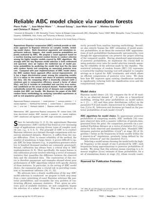
- 50. cation error by the posterior distribution; [1] is called the posterior error rate. + + + + +++ + + + + + + + + + + + + + + + + + + + + + + + + + + + + + + + + + + + + + + + + + + + + + + + + + + + + + + + + + + + + + + + + + + + + + + + + ++ + + + + + + + + + + + + + + + + ++ + + + + + + + + + ++ + + + + + + + + + + + + + + + + + + + + + + + + + + + + + + + + + + + + + ++ + + + + + + + + + + + + + + + + + + ++ + + + + + + + + + + + + + + + + + + + + + + + + + + + + + ++ + + + + + + + + + + ++ + + + + + + + + + + + + + + + + + + + + + + + + + + + + + + + + + + + + + + + + + + + + + ++ + + + + + + + + + + + + + + + + + + + + + + + + + + + + + + + + + + + + + + + + ++ + + + + + ++ + + + + + + + + + + + + + + + + + + + + + + + + + + + + + + + + + + + + + + + + + + + + + + + + + + + + + + + + + + + + + + ++ + + + +++ + + + + + + ++ + + + + + + + + + + + + + + + + + + + + + + + + + + + + + + + + + + + + + + + + + + + + + + + + + + + + + + + + + + + + + + + + + + + + + + + + + + + + + + + + + + + + + + + + + + + + + + + + + + + + + + + + + +++ + + + + + + + + + + + + + + ++ + + + + + + + + + + + + + + + + + + + + + + + + + + + + + + + + + + + + + + + + + + + + + + + + + + + + + + + + + + + + + + + + + + + + + + + + + + + + + + + + + + + + + + + + + + ++ + + + + + + + + + + + + + + + + + + + + + + + + + + + + + + + ++ + + + + + + + + + + + + ++ + + + + + + + + + + + + + + + + + + + + + + + + + + + + + + + + + ++ + + + + + + + + + + + + + + + + + + + + + + + + + + + + ++ + + ++ + + + + + + + + + + + + + + + + + + + + + + + + + + + + + + + + + + + + + + + + + + + + + + + + + + + + + + + + + + + + + + + + + + + + + + + + + + + + + + + + + + + + + + + + + + + + + + + + + + + + + + + + + + + + ++ + + + + + + + + + + + + + + + + + + + + + + + + + + + + + + ++ + + + + + + + + + + + + + + + + + + + + + + + + + + + + + + + + + + + + + + + + + + + + + + + + + + + + + + + + + + + + + + + + + + + + + + + + + ++ + + + + + + + + + + + + + + + + + + + +++ + + + + + + + + + + + + + + + + + + + + + + + + + + + + + + + + + + + + + + + + + + + + + + + + + + + + + + + + + + + + + ++ + + + + + + + + + + + + + + + + + + + + + + + + + + + + + + + + + + + + + + + + + + + + + ++ + + + + + + + + + + + + + + + + + + + + + + + + + + + + + + + ++ + + + + + + + + + + + + + + + + + + + + + + + + + + + + + + + + + + + + + + + + + + + + + + + + + + + + + + + + + + + + + ++ + + + + + + + + + + + + + + + + + + + + + + + ++ + + + + + + + + + + + + + + + + + + + + + + + + + + + + + + + + + + + + + + + + + + + + + + + + + + + + + + + + + + + + + + + + + + + + + + + + + + + + + + + + + + + + + + + + + + + + + + + + + + + + + + + + + + + + + + + + + + + + + + + + + + + + + + + + + + + + + + + + + + + + + + + + + + + + + + + + + + + + + + + + + + + + + + + + + + + + + ++ ++ + + + + + + + + + + + + + + + + + ++ + + + + + + ++ + + + + + + + + + + + + + + + + + + ++ + + + + + + ++ + + + + + + + + + + + + + + + + + + + + + + + + + + + + + + + + + + + + + + + + + + + + + + + + + + + + + + + + + + + + + + + + + + + + + + + + + + + + + + + + + + ++ + + + + ++ + + + + + + + + + + + + + + + + + + + + + + + + + + + + + + + + + + + + + + + + + + + ++ + + + + + + + + + + + + + + + + + + + + + + + + + + + +++ + + + + + + + + + + + + + + + + + + + + + + + + + + + + + + + + + + ++ + + + + + + + + ++ + + + + + + + + + + + + + + + + + + + + + + + + + + + + + + + + + + + + + + + + + + + + + + + + + + + + + + + + + + + + + + + + + + + + ++ + + + + + + + + + + + + + + + + + + + + + + + + + + + + + + + + + + + + + + + + + + + + + + + + + + + + + + + + + + + +++ + + + + + + + + + + + + + + + + + + + + + + + + + + + + + + + + + + + + + + + + + + + + + + + + + + + + + + + + + + + + + + + + + + + + + + + + + + + + + + + + + + + + + + + + + + + + + + + + + + + + + + + + + + + + + + + + + + + + + + + + + + + + + + + + + + + + + + + + + + + + + + + + + + + + + + + + + + + + + + + + + + + + + + + + + + + + + + + + + + + + + + + + + + + + + + + + + + + + + + + + + + + + + + + + + + + + ++ + + + + + + + + + + + + + + + + + + + + + + + + + + + + + + + ++ + + + + + + + + + + + + + + + ++ + + + + + + + + + + + + ++ + + + + + + + + + + + + + + + + + + + + + + + + + + + + + + + + + + ++ + + ++ + + + + + + + + + + + + + + + + + + + + + + + + + + + + + + + + + + + + + + + + + + + + + + + + + + + + + + + + + + + + + + + + + ++ + + + + + + + + + + + + + + + + + + + + + + + + + + + + + + + + + + + + + + + + + + + + + + + + + + + + + + + + + + + + + + + + + + + + + + + + + + + + + + + + + + + + + + + + + + + + + + + + + + + + + + + + + + + + + + + + + + + + + + + + + + + + + + + + + + + + + + + + + + + + + + + + + + + + + + + + + + + + + + + + + + + + + + + + + + + + + + + + + + + + + + + + + + + + + + + + + + + + + + + + + + + + + + + + + + + + + + + + + + + + + + + + + + + + + + + + + + + + + + + + + + + + + + + + + + + + + + + + + + + + + + + + + + + + + + + + + + + + + + + + + + + + + + + + + + + + + + + + + + + + + + + + + + + + + + + + + + + + + + + + + + + + + + + + + + + + + + + + + + + + + + + + + + + + + + + + + + + + + + + + + + + + + + + + + + + + + + + ++ + + + + + + + + + + + + + + + + + + + + + + + + + + + + + + + + + + + + + + + + + + + + + + + + + + + + + + + + + + + + + + + + + + + + + + + + + + + + + + + + + + + + + + + + + + + + + + + + + + + + + + + + + + + + + + + + + + + + + + + + + + + + + + + + + + + + + + + + + + + + + + + + + + + + + + + + + + + + + + + + + + + + + + + + + + + + + + + + + + + + + + + + + + + + + + + + + + + + + + + + + + + + + + + + + + + + + + + + + + + + + + + + + + + + + + + + + + + + + + + + + + + + + + + + + + + + + + + + + + + + + + + + + + + + + + + + + + + + + + + + + + + + + + + + + + + + + + + + + + + + + ++ + + + + + + + + + + + + + + + + + + + + + + + + + + + + + + + + + + + + + + + + + + + + + + + + + + + + + + + + + + + + + + + + + + + + + + + + + + + + + + + + + + + + + + + + + + + + + + + + + + + + + + + + + + + ++ + + + + + + + + + + + + + + + + + + + + + + + + + + + + + + + + + + + + + + + + + + + + + + + +++ + + + + + + + + + + + + + + + + + + + + + + + + + + + + + + + + + + + + + + + + + + + + + + + + + + + + + + + ++ + + + + + + + + + + + + + + + + + + + + ++ + + + + + + + + + + + + + + + + + + + + + + + + + + + + + + + + + + + + + + + + + + + + + + + + + ++ + + + + + + + + + + + + + + + + + + + + + + + + + + + + + + + + + + + + + + + + + + ++ + + + + + + + + + + + + + + + + + + + + + + + + + ++ + + + + ++ + + + + + + + + + + + + + + + + + + + + + + + + ++ + + + + + + + + + + + + + + + + + ++ + + + + + + + + + + + ++ + + + + + + + + + + + + + + + + + + + + + + + + + + + + + + + + + + + + + + + + + + + + + + + + + + + + + + + + + + + + + + + + + + + + + + + + + + + + + + ++ + + + + + + + + + + + + + + + + + + ++ + + + + + + + + + + + + + + + + + + + + + + ++ + + + + + + + + + + + + + + + + + + ++ + + + + + + + + + + + + + + + + + + + + + + + + + + + + + + + + + + + + + + + + + + + + + + + + + + + + + + + + + + + + + + + + + + + + + + + + + + + + + + + + + + + + + + + + + + + + + + + + + + + + + + + + + + + + + + + + + + + + + + + + + + + + + + + + + + + + + + + + + + + + + + + + + + + + + + + + + + + + + + + + + + + + + + + + + + + + + + + + + + + + + + + + + + + + + + + + + + + + + + + + + + + + + + + + + + + + + + + + + + + + + + + + + + + + + + + + ++ + + + + ++ + + + + + + + + + + + + + + + + + + + + + + + + + + ++ + + + + + + + + + + + + + + + + + + + + + + + + + + + + + + + + + + + + + + + + + + + + + + + + + + + + + + 0.0 0.2 0.4 0.6 0.8 1.0 0.0 0.2 0.4 0.6 0.8 1.0 True posterior probability of MA(2) ABC posterior probability of MA(2) Fig. 1: Illustration of the discrepancy between true posterior probabilities and their ABC approxima- tions. The aim is to choose between two nested time series models, namely moving averages of order 1 and 2 (denoted MA(1) and MA(2) respectively; see SI for more details). Each point of the plot gives the two posterior probabilities of MA(2) for a dataset simulated either from the
- 51. rst (blue) or second model (orange). Even though the
- 52. rst two autocovariance statistics are informative for this model choice, values on the x-axis, equal to the exact posterior probabilities of MA(2), dif- fer substantially from their ABC counterparts on the y-axis. The practical derivation of the posterior error rate is easily conducted via a secondary ABC algorithm, described below (see Algorithm 2). This algorithm relies on a natural prox- imity between s0 and S(y) stemming from the RF, namely the number of times both inputs fall into the same tip of an RF tree. The sample (m; ; S(y)) of size k Npp produced in step (c) constitutes an ABC approximation of the posterior predictive distribution. The posterior error rate [1] is then approximated in step (d) by averaging prediction errors over this sample. Algorithm 2 Computation of the posterior error (a) Use the trained RF to compute proximity between each (m; ; S(x)) of the reference table and s0 = S(x0) (b) Select the k simulations with the highest proximity to s0 (c) For each (m; ) in the latter set, compute Npp new simu- lations S(y) from f(yj;m) (d) Return the frequency of erroneous RF predictions over these k Npp simulations Illustrations To illustrate the power of the ABC-RF methodology, we now report several controlled experiments as well as two genuine population genetic examples. Insights from controlled experiments. SI details controlled ex- periments on a toy problem, comparing MA(1) and MA(2) time-series models, and two controlled synthetic examples from population genetics, based on SNP and microsatellite data. The toy example is particularly revealing of the dis- crepancy between the posterior probability of a model and the version conditioning on the summary statistics s0. Fig. 1 shows how far from the diagonal are realizations of the pairs ((mjx0); (mjs0)), even though the autocorrelation statistic is quite informative (8). Note in particular the vertical accu- mulation of points near p(m = 2jx0) = 1. Table S1 demon- strates the further gap in predictive power for the full Bayes solution with a true error rate of 12% versus the best solution (RF) based on the summaries barely achieving a 17% error rate. For both controlled genetics experiments in SI, the com- putation of the true posterior probabilities of the three models is impossible. The predictive performances of the competing classi
- 53. ers can nonetheless be compared on a test sample. Re- sults, summarized in Table S2 and S3 in the SI legitimate our Table 1: Harlequin ladybird data: estimated prior error rates for various classi
- 54. cation methods and sizes of reference table. Classi
- 55. cation method Prior error rates (%) trained on Nref = 10; 000 Nref = 20; 000 Nref = 50; 000 linear discriminant analysis (LDA) 39:91 39:30 39:04 standard ABC (k-nn) on DIYABC summaries 57:46 53:76 51:03 standard ABC (k-nn) on LDA axes 39:18 38:46 37:91 local logistic regression on LDA axes 41:04 37:08 36:05 random forest (RF) on DIYABC summaries 40:18 38:94 37:63 RF on DIYABC summaries and LDA axes 36:86 35:62 34:44 Performances of classi
- 56. ers used in stage (B) of Algorithm 1. A set of 10; 000 prior simulations was use to calibrate the number of neighbors k in both standard ABC and local logistic regression, and of sub-samples Nboot for the trees of RF. Prior error rates were estimated as average misclassi
- 57. cation errors on an independent set of 10; 000 prior simulations, constant over methods and sizes of the reference tables. Pudlo, Marin et al. PNAS Issue Date Volume Issue Number 3
- 58. support of RF as the optimal classi
- 59. er, with gains of several percents. Those experiments demonstrate in addition that the posterior error rate can highly vary compared with the average prior rate, hence making a case of its signi
- 60. cance in data
- 61. tting (for details, see Section 3 in the SI). A last feature worth mentioning is that, while LDA alone does not perform uniformly well over all examples, the conjunction of LDA and RF always produces improvement, with the
- 62. rst LDA axes appearing within the most active summaries of the trained forests (Fig. S6 and S8). This stresses both the ap- peal of LDA as extra summaries and the amalgamating eect of RF, namely its ability to incorporate highly relevant statis- tics within a wide set of possibly correlated or non-informative summaries. Microsatellite dataset: retracing the invasion routes of the Harlequin ladybird.The original challenge was to conduct inference about the introduction pathway of the invasive Harlequin ladybird (Harmonia axyridis) for the
- 63. rst recorded outbreak of this species in eastern North America. The dataset,
- 64. rst analyzed in (31) and (23) via ABC, includes sam- ples from
- 65. ve natural and biocontrol populations genotyped at 18 microsatellite markers. The model selection requires the formalization and comparison of 10 complex competing sce- narios corresponding to various possible routes of introduction (see analysis 1 in (31) and SI for details). We now compare our results from the ABC-RF algorithm with other classi
- 66. ca- tion methods and with the original solutions by (31) and (23). RF and other classi
- 67. ers discriminating among the 10 scenar- ios were trained on either 104, 2 104 or 5 104 simulated datasets. We included all summary statistics computed by the DIYABC software for microsatellite markers (29), namely 130 statistics, complemented by the nine LDA axes as additional summary statistics. More details about this example can be found in the SI. In this example, discriminating among models based on the observation of summary statistics is dicult. The over- lapping groups of Fig. S10 in the SI re ect that diculty, which source is the relatively low information carried by the 18 autosomal microsatellite loci considered here. Prior error rates of learning methods on the whole reference table are given in Table 1. As expected in such high dimension settings (19, Section 2.5), k-nn classi
- 68. ers behind the standard ABC methods perform uniformly badly when trained on the 130 numerical summaries, even when well calibrated. On a much smaller set of covariates, namely the nine LDA axes, these local methods (standard ABC, and the local logistic regres- sion) behave much more nicely. The best classi
- 69. er in term of prior error rates is a RF trained on the 130 summaries and the nine LDA axes, whatever the size of the reference table. Additionally, Fig. S11 shows that RFs are clearly able to au- tomatically determine the (most) relevant statistics for model comparison, including in particular some crude estimates of admixture rate de
- 70. ned in (32), some of them not selected by the experts in (31). We stress here that the level of informa- tion of the summary statistics displayed in Fig. S11 is relevant for model choice but not for parameter estimation issues. In other words, the set of best summaries found with ABC-RF should not be considered as an optimal set for further pa- rameter estimations under a given model with standard ABC techniques (3). The evolutionary scenario selected by our RF strategy fully agrees with the earlier conclusion of (31), based on ap- proximations of posterior probabilities with local logistic re- gression solely on the LDA axes (i.e., the same scenario dis- plays the highest ABC posterior probability and the largest number of selection among the decisions taken by the aggre- gated trees of RF). Another noteworthy feature of this re- analysis is the posterior error rate of the best ABC-RF, ap- proximated by 40% when running Algorithm 2 on k = 500 neighbors and Npp = 20 simulated datasets per neighbor. In agreement with this, the posterior probability bearing the cho- sen scenario in (31) is relatively low (about 60%). It is worth stressing here that posterior error rate and posterior proba- bilities are not commensurable, i.e. they cannot be measured on the same scale. For instance, a posterior probability of 60% is not the equivalent of a posterior error rate of 40%, as −5 0 5 LD1 −10 −5 0 5 10 LD2 * −10 −5 0 5 10 −10 −5 0 5 LD1 LD3 * −5 0 5 −10 −5 0 5 LD2 LD3 * −10 −5 0 5 10 −10 −5 0 5 LD1 LD4 * Fig. 2: Human SNP data: projection of the reference table on the
- 71. rst four LDA axes. Colors correspond to model in- dices. (See SI for the description of the models.) The location of the additional datasets is indicated by a large black star. Table 2: Human SNP data: estimated prior error rates for classi
- 72. cation methods and three sizes of reference table. Classi
- 73. cation method Prior error rates (%) trained on Nref = 10; 000 Nref = 20; 000 Nref = 50; 000 linear discriminant analysis (LDA) 9:91 9:97 10:03 standard ABC (k-nn) using DYIABC summaries 23:18 20:55 17:76 standard ABC (k-nn) using only LDA axes 6:29 5:76 5:70 local logistic regression on LDA axes 6:85 6:42 6:07 random forest (RF) using DYIABC initial summaries 8:84 7:32 6:34 RF using both DYIABC summaries and LDA axes 5:01 4:66 4:18 Same comments as in Table 1. 4 www.pnas.org/cgi/doi/10.1073/pnas.xxx Pudlo, Marin et al.
- 74. the former is a transform of a vector of evidences, while the latter is an average performance over hypothetical datasets. These quantities are therefore not to be assessed on the same ground, one being a Bayesian construct of the probability of a model, the other one a weighted evaluation of the chances of selecting the wrong model. SNP dataset: inference about Human population history. Because ABC-RF performs well with a substantially lower number of simulations compared to standard ABC methods, it is expected to be of particular interest for the statistical processing of massive Single Nucleotide Polymorphism (SNP) datasets, whose production is on the increase in the
- 75. eld of population genetics. We analyze here a dataset including 50,000 SNP markers genotyped in four Human populations (33). The four populations include Yoruba (Africa), Han (East Asia), British (Europe) and American individuals of African Ancestry, respectively. Our intention is not to bring new insights into Human population history, which has been and is still studied in greater details in research using genetic data, but to illustrate the potential of ABC-RF in this con- text. We compared six scenarios (i.e. models) of evolution of the four Human populations which dier from each other by one ancient and one recent historical events: (i) a single out- of-Africa colonization event giving an ancestral out-of-Africa population which secondarily split into one European and one East Asian population lineages, versus two independent out- of-Africa colonization events, one giving the European lineage and the other one giving the East Asian lineage; (ii) the pos- sibility of a recent genetic admixture of Americans of African origin with their African ancestors and individuals of Euro- pean or East Asia origins. The SNP dataset and the compared scenarios are further detailed in the SI. We used all the sum- mary statistics provided by DIYABC for SNP markers (29), namely 130 statistics in this setting complemented by the
- 76. ve LDA axes as additional statistics. To discriminate among the six scenarios of Fig. S12 in SI, RF and others classi
- 77. ers have been trained on three nested reference tables of dierent sizes. The estimated prior error rates are reported in Table 2. Unlike the previous example, the information carried here by the 50; 000 SNP markers is much higher, because it induces better separated simulations on the LDA axes (Fig. 2), and much lower prior error rates (Table 2). Even in this case, RF using both the initial sum- maries and the LDA axes provides the best results. ABC-RF on the Human dataset selects Scenario 2 as the forecasted scenario, an answer which is not visually obvious on the LDA projections of Fig. 2. But, considering previous pop- ulation genetics studies in the
- 78. eld, it is not surprising that this scenario, which includes a single out-of-Africa coloniza- tion event giving an ancestral out-of-Africa population with a secondarily split into one European and one East Asian pop- ulation lineage and a recent genetic admixture of Americans of African origin with their African ancestors and European individuals, was selected among the six compared scenarios. This selection is associated with a high con
- 79. dence level as in- dicated by an estimated posterior error rate equals to zero. As in the previous example, we used Algorithm 2 with k = 500 neighbors and then simulated Npp = 20 replicates per neigh- bor to estimate the posterior error rate. Computation time is a particularly important issue in the present example. Simulating the 10; 000 SNP datasets used to train the classi
- 80. cation methods requires seven hours on a computer with 32 processors (Intel Xeon(R) CPU 2GHz). In that context, we are delighted to observe that the RF classi-
- 81. er constructed on the summaries and the LDA axes and a 10; 000 reference table has a smaller prior error rate than all other classi
- 82. ers, even when they are trained on a 50; 000 refer- ence table. It is worth noting that standard ABC treatments for model choice are based in practice on reference tables of substantially larger sizes: 105 to 106 simulations per scenario (23, 34). For the above setting in which six scenarios are com- pared, standard ABC treatments would request a minimum computation time of 17 days (using the same computation re- sources). According to the comparative tests that we carried out on various example datasets, we found that RF globally allowed a minimum computation speed gain around a factor of 50 in comparison to standard ABC treatments (see also Sec- tion 4 of SI for other considerations regarding computation speed gain). Conclusion The present paper is purposely focused on selecting a model, which is a classi
- 83. cation problem trained on ABC simulations. Indeed, there exists a fundamental and numerical discrep- ancy between genuine posterior probabilities and probabilities based on summary statistics (10, 11). When statistics follow the consistency conditions of (12), the discrepancy remains, but the resulting algorithm asymptotically select the proper model as the size of the data grows. We defend here the paradigm shift of quantifying our con-
- 84. dence in the selected model by the computation of a poste- rior error rate, along with the abandonment of approximating posterior probabilities since the latter cannot be assessed at a reasonable computational cost. The posterior error rate pro- duces an estimated error as an average over the a posteriori most likely part of the parameter space, including the infor- mation contained in the data. It further remains within the Bayesian paradigm and is a convergent evaluation of the true error made by RF itself, whence represents a natural substi- tute to the usually uncertain ABC approximation of posterior probabilities. Compared with past ABC implementations, ABC-RF of- fers improvements at least at
- 85. ve levels: (i) on all experi- ments we studied, it has a lower prior error rate; (ii) it is robust to the size and choice of summary statistics, as RF can handle many super uous statistics with no impact on the performance rates (which mostly depend on the intrinsic di- mension of the classi
- 86. cation problem (27, 28), a characteristic con
- 87. rmed by our results); (iii) the computing eort is consid- erably reduced as RF requires a much smaller reference table compared with alternatives (i.e., a few thousands versus hun- dred thousands to billions of simulations); (iv) the method is associated with an embedded and free error evaluation which assesses the reliability of ABC-RF analysis; and (v) RF can be easily and cheaply calibrated (with no further simulations) from the reference table via the reliable out-of-bag error. As a consequence, ABC-RF allows for a more robust handling of the degree of uncertainty in the choice between models, pos- sibly in contrast with earlier and over-optimistic assessments. Due to a massive gain in computing and simulation eorts, ABC-RF will undoubtedly extend the range and complexity of datasets (e.g. number of markers in population genetics) and models handled by ABC. Once a given model has been chosen and con
- 88. dence evaluated by ABC-RF, it becomes pos- sible to estimate parameter distribution under this (single) model using standard ABC techniques (e.g. 35) or alternative methods such as those proposed by (36). ACKNOWLEDGMENTS. The use of random forests was suggested to JMM and CPR by Bin Yu during a visit at CREST, Paris, in 2013. We are grateful to our col- leagues at CBGP for their feedback and support, to the Department of Statistics at Pudlo, Marin et al. PNAS Issue Date Volume Issue Number 5
- 89. Warwick for its hospitality, and to G. Biau for his help about the asymptotics of ran- dom forests. Some parts of the research was conducted at BIRS, Ban, Canada, and the authors (PP and CPR) took advantage of this congenial research environment. The authors also acknowledge the independent research conducted on classi
- 90. cation tools for ABC by M. Gutmann, R. Dutta, S. Kaski, and J. Corander. References 1. Tavare S, Balding D, Grith R, Donnelly P (1997) Inferring coalescence times from DNA sequence data. Genetics 145:505{ 518. 2. Pritchard J, Seielstad M, Perez-Lezaun A, Feldman M (1999) Population growth of human Y chromosomes: a study of Y chromosome microsatellites. Mol. Biol. Evol. 16:1791{1798. 3. Beaumont M, Zhang W, Balding D (2002) Approximate Bayesian computation in population genetics. Genetics 162:2025{2035. 4. Beaumont M (2008) in Simulations, Genetics and Human Pre- history, eds Matsumura S, Forster P, Renfrew C (Cambridge: (McDonald Institute Monographs), McDonald Institute for Ar-chaeological Research), pp 134{154. 5. Toni T, Welch D, Strelkowa N, Ipsen A, Stumpf M (2009) Approximate Bayesian computation scheme for parameter in-ference and model selection in dynamical systems. Journal of the Royal Society Interface 6:187{202. 6. Beaumont M (2010) Approximate Bayesian computation in evolution and ecology. Annual Review of Ecology, Evolution, and Systematics 41:379{406. 7. Csillery K, Blum M, Gaggiotti O, Francois O (2010) Approxi-mate Bayesian computation (ABC) in practice. Trends in Ecol- ogy and Evolution 25:410{418. 8. Marin J, Pudlo P, Robert C, Ryder R (2011) Approximate Bayesian computational methods. Statistics and Computing pp 1{14. 9. Blum M, Nunes M, Prangle D, Sisson S (2013) A compar-ative review of dimension reduction methods in Approximate Bayesian Computation. Stat Sci 28:189{208. 10. Didelot X, Everitt R, Johansen A, Lawson D (2011) Likelihood-free estimation of model evidence. Bayesian Analysis 6:48{76. 11. Robert C, Cornuet JM, Marin JM, Pillai N (2011) Lack of con
- 91. dence in ABC model choice. Proceedings of the National Academy of Sciences 108(37):15112{15117. 12. Marin J, Pillai N, Robert C, Rousseau J (2014) Relevant statis-tics for Bayesian model choice. J Roy Stat Soc B (to appear). 13. Breiman L (2001) Random forests. Machine Learning 45:5{32. 14. Berger J (1985) Statistical Decision Theory and Bayesian Analysis (Springer-Verlag, New York), Second edition. 15. Robert C (2001) The Bayesian Choice (Springer-Verlag, New York), second edition. 16. Grelaud A, Marin JM, Robert C, Rodolphe F, Tally F (2009) Likelihood-free methods for model choice in Gibbs random
- 92. elds. Bayesian Analysis 3(2):427{442. 17. Biau G, Cerou F, Guyader A (2014) New insights into Approx-imate Bayesian Computation. Annales de l'IHP (Probability and Statistics). 18. Stoehr J, Pudlo P, Cucala L (2014) Adaptive ABC model choice and geometric summary statistics for hidden Gibbs random
- 93. elds. Statistics and Computing pp 1{13. 19. Hastie T, Tibshirani R, Friedman J (2009) The elements of statistical learning. Data mining, inference, and prediction., Springer Series in Statistics (Springer-Verlag, New York), 2 edition. 20. Freund Y, Schapire RE, et al. (1996) Experiments with a new boosting algorithm Vol. 96, pp 148{156. 21. Aeschbacher S, Beaumont MA, Futschik A (2012) A novel approach for choosing summary statistics in Approximate Bayesian Computation. Genetics 192:1027{1047. 22. Prangle D, Blum MGB, Popovic G, Sisson SA (2013) Diag-nostic tools of approximate Bayesian computation using the coverage property. ArXiv e-prints. 23. Estoup A, et al. (2012) Estimation of demo-genetic model prob-abilities with Approximate Bayesian Computation using linear discriminant analysis on summary statistics. Molecular Ecology Ressources 12:846{855. 24. Devroye L, Gyor
- 94. L, Lugosi G (1996) A probabilistic theory of pattern recognition, Applications of Mathematics (New York) (Springer-Verlag, New York) Vol. 31, pp xvi+636. 25. Breiman L (1996) Bagging predictors. Mach Learn 24:123{140. 26. Breiman L, Friedman J, Stone CJ, Olshen RA (1984) Classi
- 95. - cation and regression trees (CRC press). 27. Biau G (2012) Analysis of a random forest model. Journal of Machine Learning Research 13:1063{1095. 28. Scornet E, Biau G, Vert JP (2014) Consistency of random forests., (arXiv), Technical Report 1405.2881. 29. Cornuet JM, et al. (2014) DIYABC v2.0: a software to make Approximate Bayesian Computation inferences about popula-tion history using Single Nucleotide Polymorphism, DNA se-quence and microsatellite data. Bioinformatics (to appear). 30. Cleveland W (1979) Robust locally weighted regression and smoothing scatterplots. J Am Stat Assoc 74:829{836. 31. Lombaert E, Guillemaud T, Thomas C, et al. (2011) Infer-ring the origin of populations introduced from a genetically structured native range by Approximate Bayesian Computa-tion: case study of the invasive ladybird Harmonia axyridis. Molecular Ecology 20:4654{4670. 32. Choisy M, Franck P, Cornuet JM (2004) Estimating admixture proportions with microsatellites: comparison of methods based on simulated data. Mol Ecol 13:955{968. 33. 1000 Genomes Project Consortium, Abecasis G, Auton A, et al. (2012) An integrated map of genetic variation from 1,092 hu-man genomes. Nature 491:56{65. 34. Bertorelle G, Benazzo A, Mona S (2010) ABC as a exible framework to estimate demography over space and time: some cons, many pros. Mol Ecol 19:2609{2625. 35. Beaumont M, Zhang W, Balding D (2002) Approximate Bayesian computation in population genetics. Genetics 162:2025{2035. 36. Excoer L, Dupanloup I, Huerta-Sanchez E, Sousa V, Foll M (2013) Robust demographic inference from genomic and SNP data. PLoS Genet p e1003905. 6 www.pnas.org/cgi/doi/10.1073/pnas.xxx Pudlo, Marin et al.
- 96. Reliable ABC model choice via random forests | Supporting Information Pierre Pudlo y, Jean-Michel Marin y , Arnaud Estoup z, Jean-Marie Cornuet z , Mathieu Gautier z , and Christian P. Robert x { Universite de Montpellier 2, I3M, Montpellier, France,yInstitut de Biologie Computationnelle (IBC), Montpellier, France,zCBGP, INRA, Montpellier, France,xUniversite Paris Dauphine, CEREMADE, Paris, France, and {University of Warwick, Coventry, UK Table of contents 1. Classi
- 97. cation methods 1 2. A revealing toy example: MA(1) versus MA(2) models 3 3. Examples based on controlled simulated population genetic datasets 5 4. Supplementary information about the Harlequin ladybird example 9 5. Supplementary informations about the Human population example 13 6. Computer software and codes 15 7. Summary statistics available in the DIYABC software 16 1. Classi
- 99. cation methods aim at forecasting a variable Y that takes values in a
- 100. nite set, e.g. f1; : : : ;Mg, based on a pre-dicting vector of covariates X = (X1; : : : ;Xd) of dimension d. They are
- 101. tted with a training database (xi; yi) of indepen-dent replicates of the pair (X; Y ). We exploit such classi
- 102. ers in ABC model choice by predicting a model index (Y ) from the observation of summary statistics on the data (X). The classi
- 103. ers are trained with numerous simulations from the hi-erarchical Bayes model that constitute the ABC reference ta-ble. For a more detailed entry on classi
- 104. cation, we refer the reader to the entry (1) and to the more theoretical (2). Standard classi
- 105. ers. Discriminant analysis covers a
- 106. rst family of classi
- 107. ers including linear discriminant analysis (LDA) and nave Bayes. Those classi
- 108. ers rely on a full likelihood function corresponding to the joint distribution of (X; Y ), speci
- 109. ed by the marginal probabilities of Y and the conditional density f(xjy) of X given Y = y. Classi
- 110. cation follows by ordering the probabilities Pr(Y = yjX = x). For instance, linear dis-criminant analysis assumes that each conditional distribution of X is a multivariate Gaussian distribution with unknown mean and covariance matrix, when the covariance matrix is assumed to be constant across classes. These parameters are
- 111. tted on a training database by maximum likelihood; see e.g. Chapter 4 of (1). This classi
- 112. cation method is quite popu-lar as it provides a linear projection of the covariates on a space of dimension M 1, called the LDA axes, which sep-arate classes as much as possible. Similarly, nave Bayes as-sumes that each density f(xjy), y = 1; : : : ;M, is a product of marginal densities. Despite this rather strong assumption of conditional independence of the components of X, nave Bayes often produces good classi
- 113. cation results. Note that one can assume that the marginals are univariate Gaussians and
- 114. t those by maximum likelihood estimation, or else resort to a nonparametric kernel density estimator to recover these marginal densities when the training database is large enough. Logistic and multinomial regressions use a conditional like-lihood based on a modeling of Pr(Y = yjX = x), as special cases of a generalized linear model. Modulo a logit transform (p) = logfp=(1 p)g, this model assume linear dependency in the covariates; see e.g. Chapter 4 in (1). Logistic regres-sion results rarely dier from LDA estimates since the decision boundaries are also linear. The sole dierence stands with the procedure used to
- 115. t the classi
- 116. ers. Local methods. k-nearest neighbor (k-nn) classi
- 117. ers require no model
- 118. tting but mere computations on the training database. More precisely, it builds upon a distance on the feature space, X 3 X. In order to make a classi
- 119. cation when X = x, k-nn derives the k training points that are the closest in distance to x and classi
- 120. es this new datapoint x according to a major-ity vote among the classes of the k neighbors. The accuracy of k-nn heavily depends on the tuning of k, which should be calibrated, as explained below. Local logistic (or multinomial) regression adds a linear re-gression layer to these procedures and dates back to (3). In order to make a decision at X = x, given the k nearest neigh-bors in the feature space, one weights them by a smoothing kernel (e.g., the Epanechnikov kernel) and a multinomial clas-si
- 121. er is then
- 122. tted on this weighted sub-sample of the training database. More details on this procedure can be found in (4). Likewise, the accuracy of the classi
- 123. er depends on the cali-bration of k. Random forest construction.RF aggregates decision trees built with a slight modi
- 124. cation of the CART algorithm (5). PNAS Supplementary Information 1{17
- 125. The latter procedure produces a binary tree that sets rules as labels of the internal nodes and predictions of Y as labels of the tips (terminal nodes). At a given internal node, the rule is of the form Xj t, which determines a left-hand branch ris-ing from that vertex and a right-hand branch corresponding to Xj t. To predict the value of Y when X = x from this tree means following a path from the root by applying these binary rules and returning the label of the tip at the end of the path. The randomized CART algorithm used to create the trees in the forest recursively infers the internal and terminal labels of each tree i from the root on a training database (xi; yi) as follows. Given a tree built until a node v, daughter nodes v1 and v2 are determined by partitioning the data remaining at v in a way highly correlated with the outcome Y . Practically, this means minimizing an empirical divergence criterion (the sum of impurities of the resulting nodes v1 and v2) towards se-lecting the most discriminating covariate Xj among a random subset of the covariates, of size ntry, and the best threshold t. Assuming ^p(v; y) denotes the relative frequency of y among the part of the learning database that falls at node v, N(v) the size of this part of the database, the Gini criterion we minimize is N(v1)Q(v1) + N(v2)Q(v2), where Q(vi) = MX y=1 ^p(vi; y) f1 ^p(v;y)g : (See Chapter 9 in (1) for criteria other than the Gini index above.) The recursive algorithm stops Pwhen all terminal nodes v are homogeneous, i.e., Q(v) = M y=1 ^p(v; y)f1 ^p(v; y)g = 0 and the label of the tip v is the only value of y for which ^p(v; y) = 1. This leads to Algorithm S1, whose decision boundaries are noisy but approximately unbiased. The RF algorithm aggregates randomized CART trees trained on bootstrap sub-sample of size Nboot from the origi-nal training database (i.e., the reference table in our context). The prediction at a new covariate value X = x is the most fre-quent response predicted by the trees in the forest. Three tun-ing parameters have to be calibrated: the number B of trees in the forest, the number ntry of covariates that are sampled at each node by the randomized CART, and the size Nboot of the bootstrap sub-sample. Following (6), if d is the total number of predictors, the default number of covariates ntry is p d and the default Nboot is the size of the original train-ing database. The out-of-bag error is the average number of time an observation from the training database is misclassi-
- 126. ed by trees trained on bootstrap samples that do not include this observation, and it is instrumental in tuning the above parameters. Algorithm S1 Randomized CART start the tree with a single root repeat pick a non-homogeneous tip v such that Q(v)6= 1 attach to v two daughter nodes v1 and v2 draw a random subset of covariates of size ntry for all covariates Xj in the random subset do
- 127. nd the threshold tj in the rule Xj tj that minimizes N(v1)Q(v1) + N(v2)Q(v2) end for
- 128. nd the rule Xj tj that minimizes N(v1)Q(v1) + N(v2)Q(v2) in j and set this best rule to node v until all tips v are homogeneous (Q(v) = 0) set the labels of all tips Algorithm S2 RF for classi
- 129. cation for b = 1 to B do draw a bootstrap sub-sample Z of size Nboot from the training data grow a tree Tb trained on Z with Algorithm S1 end for output the ensemble of trees fTb; b = 1 : : :Bg Notice that the frequencies of predicted responses amid the trees of Algorithm S2 do not re ect any posterior related quantities and thus should not be returned to the user. In-deed, if it is fairly easy to reach the decision y at covariate value X = x, almost all trees will produce the same prediction y and the frequency of this class y will be much higher than Pr(Y = yjX = x). The way we build a RF classi
- 130. er given a collection of sta-tistical models is to start from an ABC reference table in-cluding a set of simulation records made of model indices, parameter values and summary statistics for the associated simulated data. This table then serves as training database for a RF that forecasts model index based on the summary statistics. Once more, we stress that the frequency of each model amid the tree predictions does not re ect any poste-rior probability. We therefore propose the computation of a posterior error rate (see main text) that render a reliable and fully Bayesian error evaluation. Calibration of the tuning parameters. Many machine learning algorithms involve tuning parameters that need to be deter-mined carefully in order to obtain good results (in terms of what is called the prior error rate in the main text). Usually, the predictive performances (averaged over the prior in our context) of classi
- 131. ers are evaluated on new data (validation procedures) or fake new data (cross-validation procedures); see e.g. Chapter 7 of (1). This is the standard way to com-pare the performances of various possible values of the tuning parameters and thus calibrate these parameters. For instance, the value of k for both k-nn and local logis-tic regression, as well as Nboot of RF, need to be calibrated. But, while k-nn performances heavily depend on the value of k, the results of RF are rather stable over a large range of values of Nboot as illustrated on Fig. S1. The plots in this Figure display an empirical evaluation of the prior error rates of the classi
- 132. ers against dierent values of their tuning pa-rameter with a validation sample made of a fresh set of 104 simulations from the hierarchical Bayesian model. Because of the moderate Monte Carlo noise within the empirical error, we
- 133. rst smooth out the curve before determining the calibra-tion of the algorithms. Fig. S1 displays this derivation for the ABC analysis of the Harlequin ladybird data with ma-chine learning tools. The last case is quite characteristic of the plateau structure of errors in RFs. The validation procedure described above requires new simulations from the hierarchical Bayesian model, which we can always produce because of the very nature of ABC. But such simulations might be computationally intensive when analyzing large datasets or complex models. The cross-validation procedure is an alternative (we do not present here) while RF oers a separate evaluation procedure: it takes ad-vantage of the fact that bootstrap samples do not contain the whole reference table, leftovers being available for testing. The resulting evaluation of the prior error rate is the out-of-bag estimator, see e.g. Chapter 15 of (1). Calibration for other classi
- 134. ers involve new prior simulations or a computationally heavy cross-validation approximation of the error. Moreover, calibrating local logistic regression may prove computation-ally unfeasible since for each dataset of the validation sample 2 Pudlo, Marin et al.
- 135. (the second reference table), the procedure involves searching for nearest neighbors in the (
- 136. rst) reference table, then
- 137. tting a weighted logistic regression on those neighbors. 0 500 1000 1500 2000 2500 3000 0.56 0.60 0.64 0.68 k Prior error rate 2000 4000 6000 8000 10000 0.371 0.374 0.377 k Prior error rate 0 10000 20000 30000 40000 50000 0.36 0.38 0.40 Nboot Prior error rate Fig. S1. Calibration of k-nn, the local logistic regression, and RF. Plot of the empirical prior error rate (in black) of three classi
- 138. ers, namely k-nn (top), the local logistic regression (middle) and RF (bottom) as a function of their tuning parameter (k for the
- 139. rst two methods, Nboot for RF) when analyzing the Harlequin ladybird data with a reference table of 10; 000 simulations (top and middle) or 50; 000 simulations (bottom). To remove the noise of these estimated errors on a validation set composed of 10; 000 independent simulations, estimated errors are smoothed by a spline method that produces the red curve. The optimal values of the parameters are k = 300, k = 3; 000 and Nboot = 40; 000, respectively. 2. A revealing toy example: MA(1) versus MA(2) models Given a time series (xt) of length T = 100, we compare
- 140. ts by moving average models of order either 1 or 2, MA(1) and MA(2), namely xt = t 1t1 and xt = t 1t1 2t2 ; t N(0; 2) ; respectively. As previously suggested (7), a possible set of (insucient) summary statistics is made of the
- 141. rst two (or higher) autocorrelations, set that yields an ABC reference table of size Nref = 104 with two covariates, displayed on Fig. S2. For both models, the priors are uniform distribu-tions on the stationarity domains (8): { for MA(1), the single parameter 1 is drawn uniformly from the segment (1; 1); { for MA(2), the pair (1; 2) is drawn uniformly over the triangle de
- 142. ned by 2 1 2; 1 + 2 1; 1 2 1: In this example, we can evaluate the discrepancy between the true posterior probabilities and those based on summaries. The true marginal likelihoods can be computed by numerical integrations of dimension 1 and 2 respectively, while the poste-rior probabilities based on the summary statistics are derived from the ABC reference table by a kernel density estimation. Fig. 1 of the main text shows how dierent the (estimated) posterior probabilities are when based on (i) the whole series of length T = 100 and (ii) only the summary statistics, even though the latter remain informative about the problem. This graph induces us to caution as to the degree of approximation provided by ABC about the true posterior probabilities and it brings numerical support to the severe warnings of (9). + + + + + + + + + + + + + + + + + + + + + + + + + + + + + + + + + + + + + + + + + + + + + + + + + + + + + + + + + + + + ++ + + + + + + + + + + + + + + + + + + + + + + + + + + + + + + + + + + ++ + + + + + + + + + + + + + + + + + + + + + ++ ++ + + ++ + + + + + + + ++ + + + + + + + + + + + + + + + + + + + + + + + + + + + + + + + + + ++++ + + + + + +++ + + + + ++ + + + + + + + + + + + + + ++ + + + + + + + + + + + + + + + + + + + + + + + + + + + + + + + + + + + + + + + + + + + + + + + + + + +++ + + + + + + + + + + + + + + + + + + + ++ + + ++ + + + + + + + ++ + + + + ++ + + + + + + + + + + + + + + + + + + + + + + + + + + + + + + + + + + + + + + + + + + + + + + + + + + + + + + + + + + + + + + + + + + + + + + + + + + + + + + + + + + + + + + + + + + + + + + + + + + ++ + + + + + + + + + + + + + + + + + + + + + + + + + + + + + + + + + + + + + + + + + + + + + + + ++ + + + + + + + + + + + + + + + + + + + + + + + + + + + + + + + + + + + + + + + + + + + + + + + + + + + + + + + + + + + + + ++ + + + + + + + + + + + + + + + + + + + + + + + + + + + + + + + + + + + + + + + + + + + + + ++ + + + + + + + + + + + + + + + ++ + + + + + + + ++ + + + + + + + + + + + + + + + + + + + + + + + + + + + + + + + + + + + + + + + + ++ + + + + + + ++ + + + + + + + + + + + ++ + + + + + + + + + + + + + + + + + + + + + + + + + + + + + + ++ + + + + + + + + + + + + + + + + + + ++ + + + + + + + + + + + + + + + + + + + + + + + + + + + + + + + + + + + + + + + + + + + + + + + + + + + + + + + + + + + + + + + + + + + + + + + + + + + + + + + + + + + + + + + + + + + + ++ + + + + + + + + + + + + + + + + + + + + + + + + + + + + + + + + + + + + + + + + ++ + + ++ + + + + + + + + + + + + + + + + + + + + + + + + ++ + + + + + + + + + + + + + + + + + + + + + + + + + + + + + + + + + + + + + + + + + + + + + + + + + + + + + + + + + + + + + + + + + + ++ ++ + + + + + + + ++ + + + + + + + + + + + + ++ + + + + + + + + + + + + + + + + + + + ++ + + + + + + + + + + + + + + + + + + + + + + + + + + +++ + + + + + + + + + + + + + + + + + + + + + + + + + + + + + + + + + + + + + + + ++ + + + + + + + + + + + + + + + + + + + + + + + + + + + + + + + + + + + + + + + + + + + + + + + + + + + + + + + + + + + + + + + + + + + + + + + + + + + + + + + + + + + + + + + + + + + + + + + + + + + + + + + + + + + + + + + + + + + + + + + + + + + + + + + + + + + + + + + + + + + + + + + + + + + + + + + + + + + + + + + + + + + + + + + + + + + + + + + + + + + + + + + + + + + + + + + + + + + + + + + + + + + + + + + + + + + +++ ++ + + + + + + + + + + + + + + + + + + + + + + + + + + + + + + + + ++ + + + + + + + + + ++ + + + + + + ++ + + + + + + + + + + + + + + + + + + + + + + + + + + + + + + + + + + + + + + + + ++ + + + + + + + + + + + + + ++ + + + + + + + + + + + + + + + + + + + + + + + + + + + + + + + + + + + + + + + + + + + + + + + + + + + + + + + + + + + + + + + + + + + + ++ + + + + + + + ++ + + + + + + + + + + + + + + + + + + + + + + + + + + + + + + + + + + + + + + + + + + + + + + + + + + + + + + + + + + + + + + + + + + + + + + + + ++ + + + + + + + + + + + + + + + + + + + + + + + + + + + + + + + ++ + + + + + + + + + + + + + + + + + + + + + + + + + + + + ++ + + + + + + + + + + + + + + + + + + + + + ++ + + + + + + + + ++ + + + + + + + + ++ + + + + ++ + ++ + + + + + + + + + + + ++ + + + + + + + + + + + + + + + + + + + + + + + + + + + ++ + + + ++ + + + + + + + + + + + + + + + + + + + + + + + + + + + + + + + + + + + + + + + + + + + + + + ++ + + + + + + + + + + + + + + + + + + + + + + + + + ++ + + + + + + + + + + + + + + + + + + + + + + + + + + + + + + + + + + + + + + + + + + + + + + + + + + + + + + + + + + + + + + + + + + + + + + + + + + + + + + + + + + + + + + + + + + + + + + + + + + + + + + + + + + + + + + + + + + + + + + + ++ + + + + + + + + + + + + + + + + + + + + + + + + + + + + + ++ + + + + + ++ + + + + + ++ + + + + + + + + + + + + + + + + + + + + + + + + + + + + + + + + + + + + + + + + + + + + + + + + + + + + + ++ + + + + + + + + ++ + + + + + + + + + + + + + + + + + + + + + + ++ + + + + + + + + + + + + + + + + + + + + + + + + + + + + + + + + + + + + + + + + + + + + ++ + + + + + + + + + + + + + + + + + + + + + + + + + + + + + + + + + + + + + + + ++ + + + + + + + + + + + + + ++ ++ + + + + + + + + + + + + + + + + + + + + + + + + + + + + + + + + + + + + + + + + + + + + + + + + + + + ++ + + + + + + + + + + + + + + + + + + + + + + + + + + + + + + + + + + + + + + + + + + + ++ + + + + + + + + + ++ + + + + + + + + + + + + + + + + + + + + + + + + + + + + ++ + + + ++ ++ + + + + + + + + + + + + + + + + + + + + + + + + + + + + + + + ++ + + + + + + + + + + + + + + + + + + + + + + ++ + + + + + + + + + + + + + ++ ++ + + + + + + + + + + + + + + + + + + + + + + + + + + + + + + + + + + + + + + + + + + + + + + + + + + + + + + + + + + + + + + + + + + + + + + + + + + + + + + + + + + + ++ + + + + + + + + + + + + + + + + + + + + + ++ + + + + + + + + + + + + + + + + + + + + + + + + + + + + + + + + + + + + + + + + + + + + + + + + + + + + + + + + + + + + + ++ + + + + + + + + + + + + + + + + + + + + + + + + + + + + ++ + + + + + + + + + + + + + + + + + + + + + + + + + + + + + + + + + + + + + + + + + + ++ + + + + + + + + + + + + + + + + + + + + + + + + + + + + + + ++ + + + + + + + + + + + + +++ + + + + + + + + + ++ + + + ++ + + + + + + + + + + + + + + + + + + + + + + + + + + + + + + + + + + + ++ + + + + + + + + + + + + + + + + + + + + + + + + + + + + + + + + + + + + + + + ++ + + + + + + + + + + + + + + + + + + + + + + + + + + + + + ++ + + + + + + + + + + + + + + + + + + + + + + + + + + + + + + + + + + + ++ + + + + + + + + + + + + + + + + + + ++ + + + + + + + + + + + + + + + + + + + + + + ++ + + + + + + + + + + + + + + + + + + + + + + + + ++ + + + + + + + + ++ + ++ + + + + + + + + + + + + + + + + + + + + + + + + + + + + + + + ++ + + + + + + + + + + + + + + + + + + + + + + + + + + + + + + + + + + + + + ++++ + + + + + + + + + + + + + + + + + + ++ ++ + + + + + + + + + + + + + + + + + + + + + + + + + + + + + + + + + + + + + + + + + + + + + + + + + + + + + + + + + + + + + + + + + + ++ + + + + + + + + + + + + + + + + + + + + + + + + + + + + + ++ + + + + + + + + + + + + + + + + + + + + + + + + + + + + + + + + + + + + + + + + + + + + + + + + + + + + + + + + ++ + + + + + + + + + + ++ + + + + + + + + + + + + + + + + + + + + + +++ + + + + + + + + + + + + + + + + + + + + + + + + + + + + + + + + + + + + + + + + ++ + + ++ + + + + + + + + + + + + + + + + + + + + + + + + + + + + + + + + + + + + + + + + + + + + + + + + + + + + + + +++ + + + + ++ + + + + + + + + + + + + + + + + + + + + + + ++ + + + + + + + + + + + + + + + + + + + + ++++ + + + ++ + + + + + + + + + + + ++ + + + + + + + + + + + + + + + + + + + + + ++ + + + + + + + + + + + + + + + + + ++ + + + + + + + + + + + + + + + + + + + + + + + + + + + + + + + + + + ++ + + + + + + + + + + + ++ + + + + + + + + ++ + + + + + + + + + + + + + + + + + + ++ + + + + + + + + + + + + + + + ++ + + + + + + + + + + + + + + + + + + + + + + + + + + + + + + + + + + + + + + + + + + + + + + + + + + + + + + + ++ + + + + + + + + + + + + + + + + + + + + + + + + + + + + + + + + + + + + + + + + + ++ + + + + + + + + + + + + + + + + + + + + + + + + ++ + + + + + + + + + + + + + + + + + + + + + + + + + + + + + + + + + + + + + + + + + + + + + + + + + + + + + + + + + + + + + + + ++ + + + + + + + + ++ ++ + + + + +++ + + + + + + + + + + + + + + + + + + + + + + + + + + + + + + + + + + + + + + + + + + + + + + + + + + + + + + + + + + + + + + + + + + + + + + + + + + + + + + + + + + + + + + + −6 −4 −2 0 2 4 6 −5 0 5 10 lag−1 autocovariance lag−2 autocovariance Fig. S2. Simulated ABC reference table under model MA(1) (blue) and MA(2) (orange). Pudlo, Marin et al. PNAS Supplementary Information 3
- 143. The discrepancy between the genuine (mjx) and the ABC ersatz (mjS(x)) cannot be explained by the curse of dimensionality: the number of summary statistics is either 2 or 7. As seen in Table S1 which draws a comparison between various classi
- 144. ers, k-nn is one of the best classi
- 145. cation meth-ods. But all methods based on summaries are outperformed by the Bayes classi
- 146. er that can be computed here via approx-imations of the genuine (mjx): this ideal classi
- 147. er achieves a prior error of 12:36%. Most of the dierence between this error rate and the 17% misclassi
- 148. cation rate achieved by ABC can be traced to dierences between (mjx) and (mjS(x)) that are so large as to be on opposite sides of the threshold 0:5. Besides, as illustrated in Fig. S2, a linear separation between both models does not occur and this is re ected by the high error rates of LDA and logistic regression in both cases. The standard ABC model choice (k-nn) does really well in this ex-ample, reaching one of the lowest error rates when optimized over the number k of neighbors. Interestingly, most methods presented in Table S1 display degraded performances when moving from two to seven summary statistics. By contrast, RFs achieve the absolute minimum in this comparison and manage to take advantage of a larger set of summaries. If we now turn to the performances of the posterior version of the misclassi
- 149. cation error (computed with Algorithm 2 dis-played in the main text), Fig. S3 shows how the posterior er-ror rates vary according to the position of the two-dimensional summary statistics, with larger errors at the boundaries be-tween both models and overall for the MA(1) model. The error rates thus range from negligible to above 30% depend-ing on the summary statistic location. Table S1. Prior error rates in the MA(1) vs. MA(2) example. Classi
- 150. cation method Prior error rate (%) 2 statistics 7 statistics linear discriminant analysis (LDA) 27:43 26:57 logistic regression 28:34 27:40 nave Bayes (with Gaussian marginals) 19:52 24:40 nave Bayes (with non-parametric marginal estimates) 18:25 21:92 k-nn with k = 100 neighbors 17:23 18:37 k-nn with k = 50 neighbors 16:97 17:35 random forest 17:04 16:15 The prior error rates displayed here were com-puted as averaged misclassi
- 151. cation errors on a set of 104 simulations independent of the sim-ulation set of 104 values that trained the clas-si
- 152. ers. Summary statistics are either the
- 153. rst two or the
- 154. rst seven autocorrelations. A base-line error of 12:36% is obtained when compar-ing the genuine posterior probabilities on the whole data. −4 −2 0 2 4 6 lag−1 auto correlation ● ● ● ● ● ● ● ● ● ● ● ● ● ● ● ● ● ● ● ● ● ● ● ● ● ● ● ● ● ● ● ● ● ● ● ● ● ● ● ● ● ● ● ● ● ● ● ● ● ● ● ● ● ● Simulated from ● ● ● ● ● ● ●● ● ● ● ● ● ● ● ● ● ● ● ● ● ● ● ● ● ● ● ● ● ● ● ● ● ● ● ● ● ● ● ● ● ● ● ● ● ● ● ● ●● ● ● ● ● ● ● ● ● ● ● ● ● ● ● ● ● ● ● ● ● ● ● ● ● ● ● ● ● ● ● ● ● ● ● ● ● ● ● ● ● ● ● ● ● ● ● ● ● ● ● ● ● ● ● ● ● ● ● ● ● ● ● ● ● ● ● ● ● ● ● ● ● ● ● ● ● ● ● ● ● ● ● ● ● ● ● ● ● ● ● ● ● ● ● ● ● ● ● ● ● ● ● ● ● ● ● ● ● ● ● ● ● ● ● ● ● ● ● ● ● ● ● ● ● ● ● ● ● ● ● ● ● ● ● ● ● ● ● ● ● ● ● ● ● ● ● ● ● ● ● ● ● ● ● ● ● ● ● ● ● ● ● ● ● ● ● ● ● ● ● ● ● ● ● ● ● ● ● ● ● ● ● ● ● ● ● ● ● ● ● ● ● ● ● ● ● ● ● ● ● ● ● ● ● ● ● ● ● ● ● ● ● ● ● ● ● ● ● ● ● ● ● ● ● ● ● ● ● ● ● ● ● ● ● ● ● ● ● ● ● ● ● ● ● ● ● ● ● ● ● ● ● ● ● ● ● ● ● ● ● ● ● ● ● ● ● ● ● ● ● ● ● ● ● ● ● ● ● ● ●● ● ● ● ● ● ● ● ● ● ● ● ● ● ● ● ● ● ● ● ● ● ● ● ● ● ● ● ● ● ● ● ● ● ● ● ● ● ● ● ● ● ● ● ● ● ● ● ● ● ● ● ● ● ● ● ● ● ● ● ● ● ● ● ● ● ● ● ● ● ● ● ● ● ● ● ● ● ● ● ● ● ● ● ● ● ● ● ● ● Predictive error −4 −2 0 2 4 lag−2 auto correlation ● ● ● 0.1 0.5 0.9 ● ● MA(1) MA(2) Fig. S3. Posterior error rates in the MA(1) vs. MA(2) example. This graph displays posterior error rates for the ABC-RF Algorithm 2 of the main text when k = 100 neighbors and Npp = 10, based on 500 replicated time series simulated from priors either with the MA(1) (blue dots) or the MA(2) (orange dots) models. The dot diameter represents the posterior error rates. Large values of the posterior error concentrate around the boundary between both models; see also Fig. S2. 4 Pudlo, Marin et al.
- 155. 3. Examples based on controlled simulated population genetic datasets Pop 1 Pop 3 Pop 2 tS tA Scenario 1 Pop 1 Pop 3 Pop 2 tS tA Scenario 2 r 1-r Pop 1 Pop 3 Pop 2 tS tA Scenario 3 Fig. S4. Three competing models of historical relationships between populations of a given species. Those population models or scenarios are used for both controlled examples based on SNP and microsatellite data: (left) Model 1 where Population 3 split from Population 1, (center) Model 2 where Population 3 split from Population 2, (right) Model 3 where Population 3 is an admixture between Population 1 and Population 2. Branches in blue represent population of eective size N1, in green N2, in red N3 and in cyan N4. We now consider a basic population genetic setting ascer-taining historical links between three populations of a given species. In both examples below, we try to decide whether a third (and recent) population emerged from a
- 156. rst popula-tion (Model 1), or from a second population that split from the
- 157. rst one some time ago (Model 2), or whether this third population was a mixture between individuals from both pop-ulations (Model 3); see Fig. S4. The only dierence between both examples stands with the kind of data they consider: the 1; 000 genetic markers of the
- 158. rst example are autosomal, sin-gle nucleotide polymorphims (SNP) loci and the 20 markers of the second example are autosomal microsatellite loci. We assume that, in both cases, the data were collected on samples of 25 diploid individuals from each population. Simulated and observed genetic data are summarized with the help of a few statistics described in Section 7 of the SI. They are all com-putable with the DIYABC software (10) that we also used to produce simulated datasets; see also Section 6. For both examples, the seven demographics parameters of the Bayesian model are { tS: time of the split between Populations 1 and 2, { tA: time of the appearance of Population 3, { N1, N2, N3: eective population sizes of Populations 1, 2 and 3, respectively, below time tS, { N4: eective population size of the common ancestral pop-ulation above tS and { r: the probability that a gene from Population 3 at time tA came from Population 1. This last parameter r is the rate of the admixture event at time tA and as such speci
- 159. c to Model 3. Note that Model 3 is equivalent to Model 1 when r = 1 and to Model 2 when r = 0. But the prior we set on r avoids nested models. Indeed, the prior distribution is as follows: { the times tS and tA (on the scale of number of generations) are drawn from a uniform distribution over the segment [10; 3 104] conditionally on tA tS; { the four eective population sizes Ni, i = 1; : : : ; 4 are drawn independently from a uniform distribution on a range from 100 to 30; 000 diploid individuals, denoted U(100; 3 104); { the admixture rate r is drawn from a uniform distribution U(0:05; 0:95). In this example, the prior on model indices is uniform so that each of the three models has a prior probability of 1=3. SNP data.The data is made of 1; 000 autosomal SNPs for which we assume that the distances between these loci on the genome are large enough to neglect linkage disequilibrium and hence consider them as having independent ancestral genealo-gies. We use all summary statistics oered by the DIYABC software for SNP markers (10), namely 48 summary statistics in this three population setting (provided in Section 7). In to-tal, we simulated 70; 000 datasets, based on the above priors. These datasets are then split into three groups: { 50; 000 datasets constitute the reference table and reserved for training classi
- 160. cation steps, (we will also consider clas-si
- 161. ers trained on subsamples of this set), { 10; 000 datasets constitute the validation set, used to cal-ibrate the tuning parameters of the classi
- 162. ers if needed, and { 10; 000 datasets constitute the test set, used to evaluating the prior error rates. The classi
- 163. cation methods applied here are given in Ta-ble S2. For the nave Bayes classi
- 164. er and the LDA procedures, there is no parameter to calibrate. The numbers k of neigh-bors for the standard ABC techniques and for the local logistic regression are tuned as described in Section 1 of the present SI. This is also the case for the size Nboot of bootstrap sub-samples in RF methods. The prior error rates are estimated and minimized by using the validation set of 104 simulations, independent from the reference table. The optimal value of k for the standard ABC (k-nn) and 48 summary statistics Pudlo, Marin et al. PNAS Supplementary Information 5
- 165. is small because of the dimension of the problem (k = 9, k = 15, and k = 55 when using 10; 000, 20; 000 and 50; 000 simulations in the reference table respectively). The optimal values of k for the local logistic regression are dierent, since this procedure
- 166. ts a linear model on weighted neighbors. The calibration on a validation set made of 10; 000 simulations produced the following optimal values: k = 2; 000, k = 3; 000, and k = 6; 000 when
- 167. tted on 10; 000, 20; 000, and 50; 000 simulations, respectively. As reported in Section 1 above, cal-ibrating the parameter k of the local logistic regression is very time consuming. In contrast, we stress that the out-of-bag er-ror rates of RF, derived directly and cheaply from the learning set (i.e., simulations from the reference table), are very close to the error rates estimated with a calibration sample. This indicates that RF does not require the simulation of a valida-tion sample, in addition to its own predictive quality, which constitutes a signi
- 168. cant computational advantage of the ap-proach. Finally, for the standard ABC (k-nn) based on orig-inal summaries, we relied on a standard Euclidean distance after normalizing each variable by its median absolute devia-tion, while k-nn on the LDA axes requires no normalization procedure. −8 −6 −4 −2 0 2 4 6 −5 0 5 10 LD1 LD2 * * Fig. S5. Projections on the LDA axes of the simulations from the reference table. Colors correspond to model indices: black for Model 1, blue for Model 2 and orange for Model 3. The locations of both simulated pseudo-observed datasets that are analyzed as if they were truly observed data, are indicated by green and red stars. Table S2 provides estimated prior error rates for those classi
- 169. cation techniques, based on a test sample of 10; 000 val-ues, independent of reference tables and calibration sets. It shows that the best error rate is associated with a RF trained on both the original DIYABC statistics and the LDA axes. The gain against the standard ABC solution is clearly sig-ni
- 170. cant. Other interesting features exhibited in Table S2 are (i) good performances of the genuine LDA method, due to a good separation between summaries coming from the three models, as exhibited in Fig. S5, albeit involving some overlap between model clusters, (ii) that the local logistic regression on the two LDA axes of (4) achieves the second best solution. Fig. S6 describes further investigations into the RF solu-tion. This graph expresses the contributions from the sum-mary statistics to the decision taken by RF. The contribution of each summary is evaluated as the average decrease in node impurity over the nodes driven by the corresponding summary statistic, see e.g. Chapter 15 of (1). The appeal of including the
- 171. rst two LDA axes is clear in Fig. S6, where they appear as LDA1 and LDA2: those statistics contribute more signif-icantly than any other statistic to the decision taken by the classi
- 172. er. Note that the FMO statistics, which also have a strong contribution to the RF decisions, are the equivalent of pairwise FST -distances between populations when genetic markers are SNPs. In order to convey the meaning of the RF posterior er-ror rate, we simulated two typical datasets, hereafter consid-ered as pseudo-observed datasets or pod(s). The
- 173. rst pod (green star in Figure S5) corresponds to a favorable situa-tion for which Model 3 should easily be discriminated from both Models 1 and 2. The parameter values used to sim-ulate this pod indeed correspond to a recent balanced ad-mixture between strongly dierentiated source populations (N1 = 20; 000, N2 = 15; 000, N3 = 10; 000, N4 = 25000, r = 0:5, ta = 500 and ts = 20000). The second pod (red star in Figure S5) corresponds to a less favorable setting where it is more dicult to discriminate Model 3 from Model 1 and 2. The parameter values used to simulate this second pod correspond to an ancient unbalanced admixture between the source populations (N1 = 20; 000, N2 = 15; 000, N3 = 10; 000, N4 = 25; 000, r = 0:1, ta = 10; 000, and ts = 20; 000). For both pods, ABC-RF (trained on both the 48 initial statistics and the two LDA axes) chooses Model 3. The RF was trained on a reference table of size 70; 000 (that con-tains all simulations) and calibrated using optimal values of Nboot = 30; 000 obtained by validation when the training set is smaller. The posterior error rates are substantially dier-ent for both pods: less than 0:1% for the
- 174. rst pod and about 12:1% for the second pod. To evaluate the Monte Carlo error of the above estimates, we repeated Algorithm 2 several times, i.e., by simulating 500 20 = 10; 000 datasets. We observed very stable posterior error rates. These posterior error rates can be compared to the 18% prior error rate of the method (see Table S2). The prior error rate is considerably higher than both posterior errors because the data space de
- 175. ned by our ABC setting includes a non-negligible proportion of worse cases, when compared with the pods represented by the green and red stars in Fig. S5. Obviously, for some less favorable cases, the posterior error rates can be higher than the prior error rate (results not shown in this case, but see the next example below based on microsatellite data). 6 Pudlo, Marin et al.
- 176. Table S2. Estimated prior error rates for the controlled SNP example. Classi
- 177. cation method Prior error rates (%) trained on Nref = 10; 000 Nref = 20; 000 Nref = 50; 000 nave Bayes (with Gaussian marginals) 34:86 34:72 34:41 linear discriminant analysis (LDA) 23:35 23:28 23:12 standard ABC (k-nn) using DIYABC summaries 27:82 25:61 23:58 standard ABC (k-nn) using only LDA axes 22:86 22:56 22:60 local logistic regression on LDA axes 22:07 21:84 21:93 random forest (RF) using DIYABC initial summaries 22:13 20:71 19:55 RF using both DIYABC summaries and LDA axes 20:07 18:95 18:11 Prior error rates are estimated by evaluating the methods (trained on three sizes of reference tables) on 10; 000 other simulations from the Bayesian model. FMO_23 FMO_13 AM1_3_12 NMO_23 NMO_13 FP0_23 FP0_13 AM1_1_23 AM1_2_13 AV1_2_13 AV1_1_23 AV1_3_12 AP0_3_12 FV1_13 NV1_13 FV1_23 NV1_23 FMO_12 FM1_23 FM1_13 l l l l l l l l l l l l l l l l l l l l 0 200 400 600 800 1000 1200 LD1 LD2 FMO_23 FMO_13 NMO_23 FP0_13 FP0_23 NMO_13 AM1_3_12 AM1_1_23 AM1_2_13 AV1_1_23 AV1_2_13 AV1_3_12 FV1_13 NV1_23 FV1_23 NV1_13 FM1_23 AP0_3_12 l l l l l l l l l l l l l l l l l l l l 0 1000 2000 3000 4000 Fig. S6. Contributions of the twenty most important statistics to the RF for the the controlled SNP example. The contribution of a statistic is evaluated as the mean decrease in node impurity in the trees of the RF when using 48 summary statistics (top) and when adding the two LDA axes to the previous set of statistics (bottom). The meaning of the variable acronyms is provided in Section 7 below. Pudlo, Marin et al. PNAS Supplementary Information 7
- 178. Microsatellite data. This illustration reproduces the same set-tings as in the SNP data example above but the genetic data (which is of much smaller dimension) carries a dierent and lower amount of information. Indeed, we consider here datasets composed of only 20 autosomal microsatellite loci. The microsatellite loci are assumed to follow a generalized stepwise mutation model with three parameters (11, 12): the mean mutation rate (), the mean parameter of the geomet-ric distribution ( P) of changes in number of repeats during mutation events, and the mean mutation rate for single nu-cleotide instability (SNI ). The prior distributions for , P and SNI are the same as those given in Table S4 (see the prior distributions used for the real Harmonia axyridis mi-crosatellite dataset). Each locus has a possible range of 40 contiguous allelic states and is characterized by locus speci
- 179. c 's drawn from a Gamma distribution with mean and shape 2, locus speci
- 180. c P's drawn from a Gamma distribution with mean P and shape 2 and,
- 181. nally, locus speci
- 182. c SNI's drawn from a Gamma distribution with mean SNI and shape 2. For microsatellite markers, DIYABC (13) produces 39 summary statistics described in Section 7 below. Table S3 is the equivalent of Table S2 for this kind of genetic data structure. Due to the lower and dierent infor-mation content of the data, the prior error rates are much higher in all cases, but the conclusion about the gain brought by RF using all summaries plus the LDA statistics remains. As in the SNP case, in order to illustrate the performances of the posterior error rate, we simulated two typical pods: one highly favorable (the green star in Fig. S7) and a second one quite challenging (the red star in Fig. S7). They were gen-erated using the same values of parameters as for the SNP pods. For both pods, we considered an ABC-RF treatment with a reference table of size 70; 000 and calibrated with Nboot = 104 as suggested by validation procedures on smaller refer-ence tables. Running twice Algorithm 2 with k = 500 nearest neighbors and Npp = 20 new simulations per neighbor, we ob-tained the following posterior error rates: about 2:5% for the
- 183. rst pod (the presumed favorable case) and about 42:5% for the second pod (the presumed challenging case). We hence obtained for the challenging pod a posterior error rate that was larger than the prior error rate. −4 −2 0 2 4 −10 −5 0 5 LD1 LD2 * * Fig. S7. Projections on the LDA axes of the simulations from the reference table. Colors correspond to model indices: black for Model 1, blue for Model 2 and orange for Model 3. The loca- tions of both simulated pseudo-observed datasets are indicated by green and red stars. Interestingly Fig. S8 shows that the AML 3 12 summary statistic (see Section 7) contributes more to the RF decision than the second LDA axis. We recall that AML is an admix-ture rate estimation computed by maximum likelihood on a simpli
- 184. ed model considering that the admixture occurred at time t = 0. The importance of the LDA axes in the random forest remains nevertheless very high in this setting. Table S3. Estimated prior error rates for the controlled SNP example. Classi