1. CENG 176A, Winter 2016
Drews, Zhang, Yang, Xu, and Vazquez-Mena
Section A02 (M/W), Team 13: The Village, Lab 3:
Efficacy of Ziegler-Nichols Tuning Method on
PID Controller for pH Control of Buffered
Solution
Part I: Alexander Michael Nootens
Part II: Edwin O. Ram´on Samayoa
Part III: Lourdes Marie Kristen Samson
Part IV: Jinyoung Choi
Abstract
Automated sustainability of a system through the use of controllers and their tuning parameters
have been proven to be extremely beneficial in a wide variety of industrial applications. In this
specific case, the pH of a solution was controlled by using a buffered solution of PBS, a computer
software controller was used to control an HCl and NaOH pump arrangement, and a pH probe
to transmit adequate pH readings. A detailed titration curve was produced in order to accurately
determine the buffer region of the solution used. Once this was complete, a generic response of the
system to P, PI, and PID control of differing tuning parameters was conducted in order to obtain
an idea of the system’s overall behavior. The ultimate period and gain were calculated by finding
the proportional band and integral time that produced a sustained oscillatory response. With these
parameters, a Ziegler-Nichols tuning method was applied to the PID controller. These tuning
parameters provided a fast rise time with minimal overshoot and zero steady state offset. These
results indicate that the Ziegler-Nichols tuning method is adequate for this specific pH control
setup to maintain the users set point pH.
2. 1 Introduction
A system controller is an electrical device that reads a process variable and alters it via a physical
output to reach a desired input set point. A common example of a current household controller
is the thermostat; the process variable is the temperature within the home and the set point is the
desired temperature set by the user. Controllers were first developed in the early 1930s when the
growing availability of electricity allowed for the promotion of industrial change and development
of automatic control.1 From then onward, controller processing units have been instrumental in
the efficiency, rate of production, and modernization of nearly all industrial disciplines.
Almost all controllers are equipped with a feedback loop that take the process variable and
compare it to the set point by measuring the difference between the two. This difference is fed
directly to the feedback controller which will apply a physical change to the desired system to
adjust the process variable back to it’s original set point. A functioning controller is able to re-
duce the magnitude of difference between the process variable and the set point rapidly while
simultaneously keeping the system stable and minimizing the steady state offset. There are three
different parameters that allow for the system control, proportional (P), integral (I), and derivative
(D) parameters.2 Proportional control decreases the time taken to reduce the error to the set point
most commonly known as the rising time. However, this type of control may increase the steady
state offset or push the system into instability. Integral control will completely remove any of the
systems steady state offset but will typically have a longer rising time, settling time, or display
oscillatory behavior. Derivative control stabilizes the system by predicting the systems response
before it has even happened.
Each individual control has positive attributes that can be used in combination with the others
in a complimentary fashion. The combination of P and I control or P, I, and D control are frequently
used depending on the response of the application they are being applied to. In order to develop
1Bennett, S., A History of Control Engineering, 1930-1955, 1st ed.; Peter Peregrinus Ltd.: United Kingdom, 1993,
pp 27–34.
2L, L. W., Process Modeling, Simulation, and Control for Chemical Engineers, 2nd ed.; McGraw Hill: New York,
1990, pp 218–231.
1
3. a control profile for a specific system there are multiple proposed tuning methods that provide
guidelines on how to determine the P, I, and D settings.
2 Background
pH control in bioreactors is an important factor for many industries such as bacteriology, baking,
brewing, and pharmaceuticals.3 Commercial applications of bioreactors maximize yield and prod-
uct output while ensuring reproducible results.4 Bioreactors must maintain an adequate pH so that
cells such as baker’s yeast and Escherichia coli grow optimally.5 The growth and metabolism of
microorganisms is especially delicate to pH.6 Integral to this ability are controllers.
Bioreactors employ P, PI, or PID controllers to maintain an optimal pH level that can save
millions of dollars by circumventing the cost of wasting a contaminated batch.7 Automated control
is better suitable for constant control due to its methodical algorithm than manual control by an
operator. For pH control, restoration of the set point requires quick response with minimal offset
in order to preserve the integrity of the biomass. The PID controller has the ability to satisfy this
requirement while utilizing the Ziegler Nichols tuning method.
Feedback control of pH to a near neutral pH level was used on a well-mixed batch system in
the following experiment to model a bioreactor. This is highly applicable to many microorganisms
because optimal growth is close to a neutral pH.8 Nonlinearities were minimized by operating in
the buffer region. To control for a lower pH, a different buffer solution should be used to reach
that level. Optimal control results should encompass low settling times, minor overshoots, and no
offsets from set point such that it can be employed in pH control of delicate biomass.
3McMillan, G. K.; Cameron, R. A., Advanced pH Measurement and Control, 3rd ed.; ISA: The Instrumentation,
Systems, and Automation Society: North Carolina, 2004, pp 3–48, 71, 199, 223.
4Lid´en, G. Understanding the bioreactor. Bioproc. Biosyst. Eng. 2002, 24, 273–279.
5Ibid.
6Rahman, M. S., Handbook of Food Preservation, 2nd ed.; CRC Press: Florida, 2007, pp 289–292.
7McMillan and Cameron, Advanced pH Measurement and Control.
8Rahman, Handbook of Food Preservation.
2
4. 3 Theory
Feedback control was employed to correct pH disturbances. The following controllers and tuning
method are generally known.9 However, these controllers are limited due to their inherent linear
properties by the Laplace transform in their derivation. Application to the non-linear process of pH
control is variable.10 Further, differences rest on the usage of a buffer solution. The buffer resists
changes in pH and serve to diminish drastic changes in pH in the buffer zone as seen in appendix
of a titration curve without buffer. This helps to linearize changes in pH and make the experiment
possible.
3.1 Linear Controller Types
There are three different controllers of interest.
The proportional (P) controller’s output is proportional to the difference between the set-point
and the controlled variable which is known as the error. It is defined in transfer function form as
Gc = Kc, (1)
where Kc is the controller gain. Note that an alternative definition of proportional band (PB)
PB =
100
Kc
(2)
is used instead of Kc, the gain. Benefits from this controller is the rapid response that increases
as the gain is set to a higher level. However, there is a limit to the gain until instabilities arise
and oscillations disrupt control of the system. Another major disadvantage is the steady state
offset from the set-point. In applications where accuracy with the desired level is important, the P
controller may be unacceptable due to its deviation from the desired set-point.
9Smith, C. A.; Corripio, A., Principles and Practice of Automatic Process Control, 3rd ed.; John Wiley and Sons:
New Jersey, 2006, pp 176–234.
10Wright, R. A.; Kravaris, C. Nonlinear Control of pH Processes Using the Strong Acid Equivalent. Ind. Eng.
Chem. Res. 1991, 30, 1561–1572.
3
5. In a proportional-integral (PI) controller, the integral of the error is taken into account for
control. It is described in transfer function form as
Gc = Kc(1+
1
τIs
), (3)
where Kc is the controller gain and τI is the time parameter, or reset time, for integral control. The
rapid response from the P control is compromised for the integral control that eliminates the steady
state offset.
The proportional-integral-derivative’s (PID) utilizes the derivative of the error in addition to
the PI control. The describing transfer function is
Gc = Kc(1+
1
τIs
+
τDs
ατDs+1
), (4)
where Kc is the controller gain, τI is the time parameter for integral control, τD is the derivative
time parameter and 1
ατDs+1 is the filter typically used during operation where α is between 0.05 and
0.2. The inclusion of a derivative parameter helps stabilize the system by anticipating the process
through the derivative of the error.
Before the controller can be employed, determination of the parameters are found through a
tuning method.
3.2 Tuning Controller Method
The Ziegler-Nichols quarter decay ratio response through ultimate gain was used. Ziegler and
Nichols determined in 1942 that the ultimate gain, Kcu, can be found by increasing the proportional
gain until marginal stability is determined while the derivative and integral portions are disabled.
From the sustained oscillations, the ultimate period of oscillation is determined. The ultimate
period is defined as,
Tu =
2π
ωu
, (5)
4
6. Table 1: Equilibrium Data
Temperature xi yi
Proportional (P) Kc = Kcu
2 − −
/ Proportional-Integral (PI) Kc = Kcu
2.2 τI = Tu
1.2 −
Proportional-Integral-Derivative (PID) Kc = Kcu
1.7 τI = Tu
2 τD = Tu
8
where ωu is the ultimate frequency. The parameters in Table 1 are used to determine the appropriate
tuning parameters for the various controllers.
The effectiveness of this method is in the simple application. By tuning the proportional gain,
the integral and derivative parameters are also derived. The quarter-decay response means that the
overshoot damps to a quarter of the amplitude in subsequent waves. This helps to minimize the
settling time, the time from when an input disturbance begins to when the signal reaches steady
state.
4 Methods
Proper personal protective equipment should be used in this lab because diluted HCl and NaOH
solutions were used. The probe was calibrated by using the provided standard buffers and pH VI.
The system should be set up as shown in Fig. 1. To create a titration curve, the pH of the PBS
buffer solution was lowered to a range of 2 to 3 and then NaOH was added slowly and constantly
to raise the pH. By doing this, the buffer region can be determined by examining the titration curve
at its most linear region. A computer software controller was used for the core experimental set
up. This software program was used to operate acid and base pumps in response to pH changes
that were different from the user specified set point. The base was fed initially because the pH was
lower than the set point pH for every trial. The set point pH was chosen within the buffer region to
allow for a less drastic change in pH per volume of acid or base added. The proportional band (P) ,
5
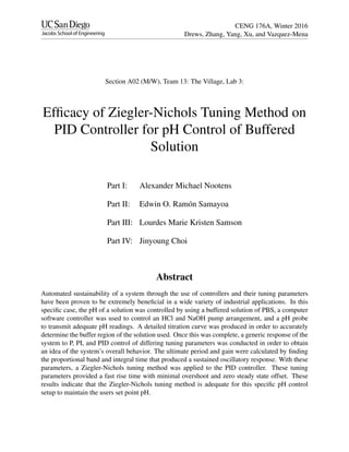
7. Figure 1: This image depicts all of the components used to deter-
mine the buffer region and allow for the pH alteration via the VI
setup ran through LabVIEW. The thin black connections between
components represent electrical connections; the thick black lines
represent tubing to allow for the transfer of acid and base respec-
tively.
Time (s)
0 50 100 150 200 250 300 350
pH
3
4
5
6
7
8
9
10
11
Figure 2: Titration curve of PBS, with NaOH titrated in. Buffer re-
gion within the pH levels of 6.25-8.35. Note: Error bars are omitted
for clarity reasons as there is a constant error of ±0.01 in the pH
levels due to the pH meter.
integral time (I), and derivative action (D) were adjusted using the provided software program. By
adjusting the three different parameters, P, PI, and PID controllers were used to determine the best
controller response and corresponding tuning parameters.
6
8. 5 Results and Discussion
A titration curve was made to find the buffer region in which the tuning parameters of the controller
were based upon. In this experiment, the buffer region was found to be between the pH range of
6.25-8.35 ±0.01 as seen in Fig. 2. A setpoint of pH 7.3 was chosen within the buffer region and
the starting pH (around pH 3) for each trial was chosen outside of the buffer region as this would
minimize the pH swing because once inside the buffer region, the tuning would stabilize quicker
with little chance of a pH swing as compared to when outside of the buffer region. From Eq. (2),
the proportional band was chosen to be 1% for all the trials because it yielded the maximum
ultimate gain the VI was capable of. Initially, we used differing values of proportional band, reset
time, and derivative action to analyze the generic response of all three tuning trials as seen in
Fig. 3. Although there was a small magnitude of overshoot the PI controller displayed the fastest
rise time as well as settling time. After the general responses were found, parameters to get the
sustained oscillations in the PI controller were extracted as seen in graph (a) of Fig. 4, and the
distance between each of the sustained oscillating peaks determined the ultimate period, Tu, of 21
seconds. Using the Ziegler-Nichols tuning relations from Table 1, specifically the equations for
Time (s)
0 20 40 60 80 100 120 140 160 180 200
pH
2
3
4
5
6
7
8
P Controller
pH Set Point
PI Controller
PID Controller
Figure 3: Comparison of the pH measurements for all three con-
troller trials based off of a trial-and-error method. Starting pH =
3.19 (P), 2.82 (PI), and 2.91 (PID), setpoint = 7.3, proportional band
= 1%, reset time = 50 sec, derivative time = 20 sec. Note: Error bars
are omitted for clarity reasons as there is a constant error of ±0.01
in the pH levels due to the pH meter.
7
9. Figure 4: (a) pH measurements for PI control trials that obtained
sustained oscillations. Starting pH = 2.93, setpoint = 7.3, propor-
tional band = 1%, reset time = 120 sec. (b) Comparison of pH
measurements for PID controller trials when based off a trial-and-
error method and the Ziegler-Nichols tuning method. Trial-and-
error method: starting pH = 2.91, setpoint = 7.3, proportional band
= 1%, reset time = 50 sec, derivative time = 20 sec. Ziegler-Nichols
method: starting pH = 2.98, setpoint = 7.3, proportional band = 1%,
reset time = 12 sec, derivative time = 3 sec. Note: Error bars are
omitted for clarity reasons as there is a constant error of ±0.01 in
the pH levels due to the pH meter.
PID, the proper reset time and derivative time were found to be 11.5 seconds and 2.625 seconds
respectively. Due to the pH controller VI parameters, the times were rounded to the nearest whole
numbers of 12 and 3. As a result, parameters for the optimized PID controller settings that were
based off of the Ziegler-Nichols tuning relations were found to have the fastest rise time and the
least steady state offset as seen in graph (b) of Fig. 4, where the gain was 58.82.
Referring back to Fig. 3, the typical behavior of a PI controller was observed, but not for the
PID controller. When there is only P control, it can typically speed up a process loop and reduce the
steady-state offset. The offset can not be eliminated with P control itself and based off the graph,
the controller seemed to act in a first order response. When integral control is added to make the
PI control, the order is increased,the offset is eliminated and P-mode speeds the response up as
shown in the graph. When the derivative control is added to make the combined PID controller,
there should be a stabilizing effect and the settling time is decreased. However that did not occur,
8
10. rather there were continuous oscillations that did not seem to settle down after an extended period
of time. This occurred because the derivative time was set to 20 seconds, thus the controller was
trying to predict the pH 20 seconds into the future causing dramatic oscillations.
As seen in graph (b) of Fig. 4, there is a significant difference between the tuned PID controller
through the Ziegler-Nichols method and the untuned PID controller that was from a trial-and-error
method. As stated earlier, the untuned PID controller gave continuous oscillations because of
the large derivative time. However, when the proper parameters were found through the Ziegler-
Nichols tuning relations, especially with a lower derivative time of 3 seconds, there was almost an
immediate rise time, when compared to the former, and a settling time of about 35 seconds. The
settling time was the fastest when compared to all of the other controller trials.
With the Ziegler-Nichols tuning relations, a quarter decay ratio response is expected and as
seen in the PID controller, the quarter decay ratio response occurred. The first overshoot was
already minimal, so the second overshoot is not noticeable at first glance; however, based off the
data points, the height between the two overshoots has the difference of 4 as a quarter decay ratio
response is expected to do.The Ziegler-Nichols tuning method provided an adequate settling time
and overall fast response to change the process variable to our setpoint.
6 Conclusion
After testing multiple different controller types with varying tuning parameters we were able to
determine the best response for our particular system. In order to do this, the ultimate period and
gain were found by obtaining sustained oscillations within the PI control. These values were used
in accordance with the Ziegler-Nichols tuning parameters to obtain a proportional band of 1%, an
integral time of 12 seconds, and a derivative time of 3 seconds. With these values we observed the
system reached the set point more quickly than any of the other trials. In addition, these tuning
values had the smallest magnitude of initial overshoot and produced zero steady state offset.
A few recommendations for future avenues of research that would improve the analysis of
9
11. this system are integrated within the methods of the data acquisition process. When creating the
titration curve, it’s important to add the NaOH solution as slowly as possible so the pH probe can
take the largest pH data sample as possible. This will allow for a detailed titration curve and a
better determination of the actual buffer region. It’s also important to make sure the solution is
well stirred to allow the pH probe to relay its readings to the controller as fast as possible. If not,
this time delay due to inadequate mixing will affect the controller response.
10
12. Appendix
Time (s)
0 20 40 60 80 100 120
pH
0
2
4
6
8
10
12
14
Figure 5: Typical titration curve of an acid with a base added. The
acid used is HCl and the base used is NaOH.
A-1