SlideShare una empresa de Scribd logo
1 de 31
Pairs Trading: Performance
of a Relative-Value Arbitrage Rule
Evan Gatev
Boston College
William N. Goetzmann
Yale University
K. Geert Rouwenhorst
Yale University
We test a Wall Street investment strategy, ‘‘pairs trading,’’ with daily data over
1962–2002. Stocks are matched into pairs with minimum distance between normal-
ized historical prices. A simple trading rule yields average annualized excess returns of
up to 11% for self-financing portfolios of pairs. The profits typically exceed conser-
vative transaction-cost estimates. Bootstrap results suggest that the ‘‘pairs’’ effect
differs from previously documented reversal profits. Robustness of the excess returns
indicates that pairs trading profits from temporary mispricing of close substitutes. We
link the profitability to the presence of a common factor in the returns, different from
conventional risk measures.
Wall Street has long been interested in quantitative methods of specula-
tion. One popular short-term speculation strategy is known as ‘‘pairs
trading.’’ The strategy has at least a 20-year history on Wall Street and
is among the proprietary ‘‘statistical arbitrage’’ tools currently used by
hedge funds as well as investment banks. The concept of pairs trading is
disarmingly simple. Find two stocks whose prices have moved together
historically. When the spread between them widens, short the winner and
buy the loser. If history repeats itself, prices will converge and the arbi-
trageur will profit. It is hard to believe that such a simple strategy, based
solely on past price dynamics and simple contrarian principles, could
possibly make money. If the U.S. equity market were efficient at all
times, risk-adjusted returns from pairs trading should not be positive.
In this article, we examine the risk and return characteristics of pairs
trading with daily data over the period 1962 through December 2002.
We are grateful to Peter Bossaerts, Michael Cooper, Jon Ingersoll, Ravi Jagannathan, Maureen O’Hara,
Carl Schecter, and two anonymous referees for many helpful discussions and suggestions on this topic.
We thank the International Center for Finance at the Yale School of Management for research support,
and the participants in the EFA’99 Meetings, the AFA’2000 Meetings, the Berkeley Program in Finance,
and the Finance and Economics workshops at Vanderbilt and Wesleyan for their comments. Address
correspondence to Evan Gatev, Boston College, Carroll School of Management, Fulton Hall, 140
Commonwealth Ave, Chestnut Hill, MA 02467, or email: gatev@bc.edu.
Ó The Author 2006. Published by Oxford University Press on behalf of The Society for Financial Studies. All rights
reserved. For permissions, please email: journals.permissions@oxfordjournals.org.
doi:10.1093/rfs/hhj020 Advance Access publication February 13, 2006
Using a simple algorithm for choosing pairs, we test the profitability of
several straightforward, self-financing trading rules. We find average
annualized excess returns of about 11% for top pairs portfolios. Although
pairs strategies exploit temporary components of stock prices, we show
that our profits are not caused by simple mean reversion as documented
in the previous literature. We examine the robustness of our results to a
wide variety of risk factors—including not only the widely used factors in
the empirical literature but also potential low-frequency institutional
factors such as bankruptcy risk. In addition, we explore the robustness
of our results to microstructure factors such as the bid-ask bounce, short-
selling costs, and transaction costs. Although some factors such as short-
selling and transaction costs affect the magnitude of the excess returns,
pairs trading remains profitable for reasonable assumptions over the
sample period of study, as well as over a true out-of-sample test of four
years. We interpret the results of our analysis as evidence in favor of
profitable arbitrage in expectations that may accrue to market partici-
pants who possess relatively low transaction costs and the ability to short
securities. We also find evidence that points to a systematic factor that
influences the profitability of pairs trading over time. This unidentified
latent risk factor has been relatively dormant recently. The importance of
this risk factor is correlated with the returns to pairs trading, which is
consistent with the view that the profits are a compensation to arbitra-
geurs for enforcing the ‘‘Law of One Price.’’
We argue that our results reveal something about the mechanism and
performance of relative-price arbitrage activities in practice. This is
potentially useful to researchers because, despite considerable theory
about market efficiency, economists have little empirical information
about how efficiency is maintained in practice. In addition, despite the
fact that hedge funds have attracted an increasing amount of investment
capital over the past decade, the study of hedge fund strategies is in its
infancy in the financial economics literature. This article examines the risk
and return characteristics of one widely practiced active trading strategy.
One natural question to ask is whether our results imply a violation of
equilibrium asset pricing. Although the documented profitability of the
pairs trading rule is a robust result, it is not inconsistent with all pricing
models. Indeed the reversion in relative values we find is consistent with a
pricing model in prices developed and tested by Bossaerts (1988). Thus,
our article at the very least suggests that this class of models merits further
empirical investigation.
The remainder of the article is organized as follows. Section 1 provides
some background on pairs trading strategy. The next section describes
our methodology of constructing pairs and calculating returns. The
empirical results are described in Section 3, and Section 4 provides con-
clusions and directions for future research.
The Review of Financial Studies / v 19 n 3 2006
798
1. Background of Pairs Trading
1.1 History
In the mid-1980s, the Wall Street quant Nunzio Tartaglia assembled a
team of physicists, mathematicians, and computer scientists to uncover
arbitrage opportunities in the equities markets. Tartaglia’s group of for-
mer academics used sophisticated statistical methods to develop high-tech
trading programs, executable through automated trading systems, which
took the intuition and trader’s ‘‘skill’’ out of arbitrage and replaced it with
disciplined, consistent filter rules. Among other things, Tartaglia’s pro-
grams identified pairs of securities whose prices tended to move together.
They traded these pairs with great success in 1987—a year when the group
reportedly made a $50 million profit for the firm. Although the Morgan
Stanley group disbanded in 1989 after a couple of bad years of perfor-
mance, pairs trading has since become an increasingly popular ‘‘market-
neutral’’ investment strategy used by individual and institutional traders
as well as hedge funds. The increased popularity of quantitative-based
statistical arbitrage strategies has also apparently affected profits. In a
New York Times interview, David Shaw, head of one of the most success-
ful modern quant shops and himself an early Tartaglia’s prote´ge´, sug-
gests that recent pickings for quant-shops have become slim—he
attributes the success of his firm, D. E. Shaw, to early entry into the
business. Tartaglia’s own explanation for pairs trading is psychological.
He claims, ‘‘... Human beings don’t like to trade against human nature,
which wants to buy stocks after they go up not down’’ [Hansell (1989)].
Could pairs traders be the disciplined investors taking advantage of the
undisciplined over-reaction displayed by individual investors? This is at
least one possible—albeit psychological—explanation for our results,
which is consistent with Jegadeesh and Titman’s (1995) finding that contra-
rian profits are in part due to over-reaction to company-specific informa-
tion shocks rather than price reactions to common factors.
1.2 Data snooping and market response
In our study we have not searched over the full strategy space to identify
successful trading rules, but rather we have interpreted practitioner
description of pairs trading as straightforwardly as possible. Our rules
follow the general outline of first ‘‘find stocks that move together,’’ and
second ‘‘take a long–short position when they diverge and unwind on
convergence.’’ A test requires that both of these steps must be parameter-
ized in some way. How do you identify ‘‘stocks that move together?’’
Need they be in the same industry? Should they only be liquid stocks?
How far do they have to diverge before a position is put on? When is a
position unwound? We have made some straightforward choices about
each of these questions. We put positions on at a two-standard deviation
Pairs Trading
799
spread, which might not always cover transaction costs even when stock
prices converge. Although it is tempting to try potentially more profitable
schemes, the danger in data-snooping refinements outweigh the potential
insights gained about the higher profits that could result from learning
through testing.1
As with all filter rules using historical asset pricing data, data snooping
is a potential concern. One approach to the data snooping issue is to test
the results out of sample. We completed and circulated the first draft of
the working paper in 1999, using data through the end of 1998. The time
lag between the first analysis and the present study gives us an ideal
holdout sample. Using the original model, but the post-1988 data, we
found that over the 1999–2002 period, the excess return of the fully
invested portfolio of the top 20 pairs averaged 10.4% per annum, with
an annual standard deviation of 3.8% and a large and significant Newey-
West-adjusted t-statistic of 4.82—consistent with the long-term, in-sample
results of our original analysis. We were careful not to adjust our strategy
from the first draft to the current draft of the article, to avoid data-
snooping criticisms. Not only does this additional four-year sample suggest
that the results were not simply an artifact of the earlier sample period, over
which pairs trading was known to be popular, but it also suggests that the
public dissemination of the results has apparently not affected the general
risk and return characteristics of the strategy, despite curiosity from the
professional sector.
1.3 Relative pricing
Asset pricing can be viewed in absolute and relative terms. Absolute
pricing values securities from fundamentals such as discounted future
cash flow. This is a notoriously difficult process with a wide margin for
error. Articles by Bakshi and Chen (1997) and Lee et al. (1997), for
example, are heroic attempts to build quantitative value-investing models.
Relative pricing is only slightly easier. Relative pricing means that two
securities that are close substitutes for each other should sell for the same
price—it does not say what that price will be. Thus, relative pricing allows
for bubbles in the economy, but not necessarily arbitrage or profitable
speculation. The Law of One Price [LOP] and a ‘‘near-LOP’’ are applic-
able to relative pricing—even if that price is wrong.
Ingersoll (1987) defines the LOP as the ‘‘proposition ... that two invest-
ments with the same payoff in every state of nature must have the same
current value.’’ In other words, two securities with the same prices in all
states of the world should sell for the same amount. Chen and Knez
(1995) extend this to argue that ‘‘closely integrated markets should assign
1
Froot and Dabora (1999) consider ‘‘twin’’ stocks that trade in different international markets to examine
the issues of market integration.
The Review of Financial Studies / v 19 n 3 2006
800
to similar payoffs prices that are close.’’ They argue that two securities
with similar, but not necessarily, matching payoffs across states should
have similar prices. This is of course a weaker condition and subject to
bounds on prices for unusual states; however, it allows the examination of
‘‘near-efficient’’ economies, or in Chen and Knez’ case, near integrated
markets. Notice that this theory corresponds to the desire to find two
stocks whose prices move together as long as we can define states of
nature as the time series of observed historical trading days.
We use an algorithm to choose pairs based on the criterion that they have
had the same or nearly the same state prices historically. We then trade
pairs whose prices closely match in historical state-space, because the LOP
suggests that in an efficient market their prices should be nearly identical. In
this framework, the current study can be viewed as a test of the LOP and
near-LOP in the U.S. equity markets, under certain stationarity conditions.
We are effectively testing the integration of very local markets—the markets
for specific individual securities. This is similar in spirit to Bossaerts’ (1988)
test of co-integration of security prices at the portfolio level. We further
conjecture that the marginal profits to be had from risk arbitrage of these
temporary deviations is crucial to the maintenance of first-order efficiency.
We could not have the first effect without the second.
1.4 Co-integrated prices
The pairs trading strategy may be justified within an equilibrium asset-pricing
framework with nonstationary common factors like Bossaerts and Green
(1989) and Jagannathan and Viswanathan (1988). If the long and short
components fluctuate with common nonstationary factors, then the prices
of the component portfolios would be co-integrated and the pairs trading
strategy would be expected to work. Evidence of exposures to common
nonstationary factors would support a nonstationary factor pricing frame-
work.
The space of normalized, cum-dividend prices, that is, cumulative total
returns with dividends reinvested, is the basic space for the pairs trading
strategies in this article. The main observation about our motivating
models of the CAPM-APT variety is that they are known to imply perfect
collinearity of prices, which is readily rejected by the data. On the other
hand, Bossaerts (1988) finds evidence of price co-integration for the U.S.
stock market. We would like to keep the notion of the empirically
observed co-movement of prices, without unnecessarily restrictive
assumptions, hence we proceed in the spirit of the co-integrated prices
literature. More specifically, our matching in price space can be inter-
preted as follows. Suppose that prices obey a statistical model of the form,
pit¼
X
ilplt þ eit; k<n ð1Þ
Pairs Trading
801
where eit denotes a weakly dependent error in the sense of Bossaerts (1988).
Assume also that pit is weakly dependent after differencing once. Under
these assumptions, the price vector pt is co-integrated of order 1 with co-
integrating rank r = n – k, in the sense of Engle and Granger (1987) and
Bossaerts (1988). Thus, there exist r linearly independent vectors {aq}q =
1,...,r such that zq = aq
0
pt are weakly dependent. In other words, r linear
combinations of prices will not be driven by the k common nonstationary
components pl. Note that this interpretation does not imply that the market
is inefficient, rather it says that certain assets are weakly redundant, so that
any deviation of their price from a linear combination of the prices of other
assets is expected to be temporary and reverting.
To interpret the pairs as co-integrated prices, we need to assume that
for n » k, there are co-integrating vectors that have only two nonzero
coordinates. In that case, the sum or difference of scaled prices will be
reverting to zero and a trading rule could be constructed to exploit the
expected temporary deviations. Our strategy relies on exactly this conclu-
sion. In principle one could construct trading strategies with trios, quad-
ruples, and so on of stocks, which would presumably capture more
co-integrated prices and would yield better profits.
The assumption that a linear combination of two stocks can be weakly
dependent may be interpreted as saying that a co-integrating vector can
be partitioned in two parts, such that the two corresponding portfolios
are priced within a weakly dependent error of another stock. Given the
large universe of stocks, this statement is always empirically valid and
provides the basis of our formation procedure.2
However, it is important
to recognize the possibility of spuriously correlated prices, which are not
de facto co-integrated.
1.5 Bankruptcy risk
The risk of bankruptcy is one reason why the returns on individual
securities cannot be taken as stationary. Sensitivity of the pairs trading
to the default premium suggests that the strategy may work because we
are pairing two firms, the first of which may have a constant or decreasing
probability of bankruptcy (short end), whereas the second may have a
temporarily increasing probability of bankruptcy (long end). The ‘‘sur-
prise improvements’’ in the short end are then followed by improvement
in the long end if that stock survives. In other words, the source of the
profit is the improving ex post (non)realization of idiosyncratic bank-
ruptcy risk in the long (loser) stock. In such case, we would expect to have
asymmetry in the profits from the long and the short components, with
2
Note that the case n » k corresponds to the standard finance paradigm where in the large universe of n
stocks, expected returns are driven by a few, namely k, common factors. This paradigm is supported by
existing empirical work, for example, see Connor and Korajczyk (1993) for references, which generally
finds less than 10 common nonstationary components.
The Review of Financial Studies / v 19 n 3 2006
802
most of the profits coming from the long end.3
We test long and short
positions separately to see if this is driving our results.
2. Methodology
Our implementation of pairs trading has two stages. We form pairs over a
12-month period (formation period) and trade them in the next 6-month
period (trading period). Both 12 months and 6 months are chosen arbi-
trarily and have remained our horizons since the beginning of the study.
2.1 Pairs formation
In each pairs formation period, we screen out all stocks from the CRSP
daily files that have one or more days with no trade. This serves to identify
relatively liquid stocks as well as to facilitate pairs formation. Next, we
construct a cumulative total returns index for each stock over the forma-
tion period. We then choose a matching partner for each stock by finding
the security that minimizes the sum of squared deviations between the two
normalized price series. Pairs are thus formed by exhaustive matching in
normalized daily ‘‘price’’ space, where price includes reinvested dividends.
We use this approach because it best approximates the description of
how traders themselves choose pairs. Interviews with pairs traders suggest
that they try to find two stocks whose prices ‘‘move together.’’ In addition
to ‘‘unrestricted’’ pairs, we will also present results by sector, where we
restrict both stocks to belong to the same broad industry categories
defined by Standard and Poors: Utilities, Transportation, Financial,
and Industrials. Each stock is assigned to one of these four groups,
based on the stock’s SIC code. The minimum-distance criterion is then
used to match stocks within each of the groups.
2.2 Trading period
Once we have paired up all liquid stocks in the formation period, we study
the top 5 and 20 pairs with the smallest historical distance measure, in
addition to the 20 pairs after the top 100 (pairs 101–120). This last set is
valuable because most of the top pairs share certain characteristics, which
will be described in detail below. On the day following the last day of the
pairs formation period, we begin to trade according to a prespecified rule.
Figure 1 illustrates the pairs trading strategy using two stocks, Kennecott
and Uniroyal, in the six-month period starting in August of 1962. The
top two lines represent the normalized price paths with dividends
reinvested and the bottom line indicates the opening and closing of the
strategy on a daily basis. It is clear why these two firms paired with each
other. They generally tended to move together over the trading interval.
3
We thank an anonymous referee for this example.
Pairs Trading
803
Notice that the position first opens in the seventh trading day of the period
and then remains open until day 36. Over that interval, the spread actually
first increased significantly before convergence. The prices remain close
during the period and cross frequently. The pair opens five times during the
period, however not always in the same direction. Neither stock is the
‘‘leader.’’ In our example, convergence occurs in the final day of the period,
although this is not always the case.
We select trading rules based on the proposition that we open a long–
short position when the pair prices have diverged by a certain amount and
close the position when the prices have reverted. Following practice, we
base our rules for opening and closing positions on a standard deviation
metric. We open a position in a pair when prices diverge by more than
two historical standard deviations, as estimated during the pairs forma-
tion period. We unwind the position at the next crossing of the prices. If
prices do not cross before the end of the trading interval, gains or losses
are calculated at the end of the last trading day of the trading interval. If a
stock in a pair is delisted from CRSP, we close the position in that pair,
using the delisting return, or the last available price.4
We report the
Figure 1
Daily normalized prices: Kennecott and Uniroyal (pair 5)
Trading period August 1963–January 1964.
4
The profits are robust with respect to this delisting assumption. A potential problem arises if inaccurate
and stale prices exaggerate the excess returns and bias the estimated return of a long position in a
plummeting stock. To address this potential concern, we have reestimated our results under the extreme
assumption that only a long stock experiences a –100% return when it is delisted. This zero-price extreme
includes, among other things, the possibility of nontrading due to the lack of liquidity. Because selective
loss on the long position always harms the pair profit, this extreme assumption biases the results against
profitability. However, pairs trading remains profitable under this alternative: for example, the average
monthly return on the top 20 pairs portfolio is 1.32% with a standard deviation of 1.9%.
The Review of Financial Studies / v 19 n 3 2006
804
payoffs by going one dollar short in the higher-priced stock and one
dollar long in the lower-priced stock.
2.3 Excess return computation
Because pairs may open and close at various points during the six-month
trading period, the calculation of the excess return on a portfolio of pairs
is a nontrivial issue. Pairs that open and converge during the trading
interval will have positive cash flows. Because pairs can reopen after
initial convergence, they can have multiple positive cash flows during
the trading interval. Pairs that open but do not converge will only have
cash flows on the last day of the trading interval when all positions are
closed out. Therefore, the payoffs to pairs trading strategies are a set of
positive cash flows that are randomly distributed throughout the trading
period, and a set of cash flows at the end of the trading interval that can
be either positive or negative. For each pair we can have multiple cash
flows during the trading interval, or we may have none in the case when
prices never diverge by more than two standard deviations during the
trading interval. Because the trading gains and losses are computed over
long–short positions of one dollar, the payoffs have the interpretation of
excess returns. The excess return on a pair during a trading interval is
computed as the reinvested payoffs during the trading interval.5
In parti-
cular, the long and short portfolio positions are marked-to-market daily.
The daily returns on the long and short positions are calculated as value-
weighted returns in the following way,
rP;t ¼
P
iEP wi;tri;t
P
iEPwi;t
ð2Þ
wi;t ¼ wi;tÀ1ð1 þ ri;tÀ1Þ ¼ ð1 þ ri;1Þ Á Á Á ð1 þ ri;tÀ1Þ ð3Þ
where r defines returns and w defines weights, and the daily returns are
compounded to obtain monthly returns. This has the simple interpreta-
tion of a buy-and-hold strategy.
We consider two measures of excess return on a portfolio of pairs: the
return on committed capital and the fully invested return, that is, the
return on actual employed capital. The former scales the portfolio payoffs
by the number of pairs that are selected for trading, the latter divides the
payoffs by the number of pairs that open during the trading period. The
former measure of excess return is clearly more conservative: if a pair
does not trade for the whole of the trading period, we still include a dollar
5
This is a conservative approach to computing the excess return, because it implicitly assumes that all cash
earns zero interest rate when not invested in an open pair. Because any cash flow during the trading
interval is positive by construction, it ignores the fact that these cash flows are received early and
understates the computed excess returns.
Pairs Trading
805
of committed capital as the cumulative return in our calculation of excess
return. It takes into account the opportunity cost of hedge funds of
having to commit capital to a strategy even if the strategy does not
trade. To the extent that hedge funds are flexible in their sources and
uses of funds, computing excess return relative to the actual capital
employed may give a more realistic measure of the trading profits.
We initiate the pairs strategy by trading the pairs at the beginning of
every month in the sample period, with the exception of the first 12
months, which are needed to estimate pairs for the strategy starting in
the first month. The result is a time series of overlapping six-month
trading period excess returns. We correct for the correlation induced
by overlap by averaging monthly returns across trading strategies that
start one month apart as in Jegadeesh and Titman (1993). The resulting
time series has the interpretation of the payoffs to a proprietary trading
desk, which delegates the management of the six portfolios to six different
traders whose formation and trading periods are staggered by one
month.
3. Empirical Results
3.1 Strategy profits
Table 1 summarizes the excess returns for the pairs portfolios that are
unrestricted in the sense that the matching stocks do not necessarily
belong to the same broad industry categories. In Section 3.5 we will
consider sector-neutral pairs strategies. Panel A summarizes the excess
returns of pairs strategies when positions are opened at the end of the day
that prices diverge and closed at the end of the day of price convergence.
The first row shows that a fully invested portfolio of the five best pairs
earned an average excess monthly return of 1.31% (t-statistic = 8.84), and
a portfolio of the 20 best pairs 1.44% per month (t = 11.56). Using the
more conservative approach to computing excess returns, using com-
mitted capital, gives excess returns of 0.78 and 0.81% per month, respec-
tively. Either way, these excess returns are large in an economical and
statistical sense and suggest that pairs trading is profitable.
The remainder of Panel A provides information about the excess return
distributions of pairs portfolios. There are diversification benefits from
combining multiple pairs in a portfolio. As the number of pairs in a
portfolio increases, the portfolio standard deviation falls. The diversifica-
tion benefits are also apparent from the range of realized returns. Inter-
estingly, as the number of pairs in the strategy increases, the minimum
realized return increases, whereas the maximum realized excess return
remains relatively stable. During the full sample period of 474 months, a
portfolio of 20 pairs experienced 71 monthly periods with negative pay-
offs, compared to 124 months for a portfolio of 5 pairs. The decrease in
The Review of Financial Studies / v 19 n 3 2006
806
the standard deviation and the increase of the lower end of the return
distribution are also reflected in an increased skewness coefficient.
Because pairs trading is in essence a contrarian investment strategy, the
returns may be biased upward because of the bid-ask bounce [Jegadeesh
(1990), Jegadeesh and Titman (1995), Conrad and Kaul (1989)]. In parti-
cular, our strategy sells stocks that have done well relative to their match
and buys those that have done poorly. Part of any observed price diver-
gence is potentially due to price movements between bid and ask quotes:
conditional on divergence, the winner’s price is more likely to be an ask
quote and the loser’s price a bid quote. In Panel A we have used these
same prices for the start of trading and our returns may be biased upward
because of the fact that we are implicitly buying at bid quotes (losers) and
selling at ask quotes (winners). The opposite is true at the second crossing
Table 1
Excess returns of unrestricted pairs trading strategies
Pairs portfolio Top 5 Top 20 101–120 All
A. Excess return distribution (no waiting)
Average excess return (fully invested) 0.01308 0.01436 0.01081 0.01104
Standard error (Newey-West) 0.00148 0.00124 0.00094 0.00099
t-Statistic 8.84 11.56 11.54 11.16
Excess return distribution
Median 0.01194 0.01235 0.00955 0.00728
Standard deviation 0.02280 0.01688 0.01540 0.01670
Skewness 0.62 1.39 1.34 3.42
Kurtosis 7.81 10.54 10.30 25.25
Minimum –0.10573 –0.06629 –0.03857 –0.02721
Maximum 0.14716 0.13295 0.12684 0.17178
Observations with excess return < 0 26% 15% 21% 17%
Average excess return on committed capital 0.00784 0.00805 0.00679 0.00614
B. Excess return distribution (one day waiting)
Average monthly return (fully invested) 0.00745 0.00895 0.00795 0.00715
Standard error (Newey-West) 0.00119 0.00096 0.00085 0.00090
t-Statistic 6.26 9.29 9.40 7.92
Excess return distribution
Median 0.00699 0.00690 0.00694 0.00411
Standard deviation 0.02101 0.01527 0.01438 0.01577
Skewness 0.34 1.45 0.98 3.32
Kurtosis 10.64 16.13 7.78 25.66
Minimum –0.12628 –0.08218 –0.04266 –0.02951
Maximum 0.14350 0.13490 0.10464 0.16325
Observations with excess return < 0 35% 23% 28% 32%
Average excess return on committed capital 0.00463 0.00520 0.00503 0.00396
Summary statistics of the monthly excess returns on portfolios of pairs between July 1963 and December
2002 (474 observations). We trade according to the rule that opens a position in a pair at the end of the
day that prices of the stocks in the pair diverge by two historical standard deviations (Panel A). The
results in Panel B correspond to a strategy that delays the opening of the pairs position by one day. All
pairs are ranked according to least distance in historical price space. The ‘‘top n’’ portfolios include the
n pairs with least distance measures, and the portfolio ‘‘101–120’’ studies the 20 pairs after the top 100.
The average number of pairs in the all-pair portfolio is 2057. The t-statistics are computed using Newey-
West standard errors with six-lag correction. Absolute kurtosis is reported.
Pairs Trading
807
(convergence): part of the drop in the winner’s price can reflect a bid
quote, and part of the rise of the loser’s price—an ask quote.
To address this issue, Panel B of Table 1 provides the excess returns
when we initiate positions in each pair on the day following the diver-
gence and liquidate on the day following the crossing. The average excess
returns on the fully invested portfolios and on committed capital drop by
about 30–55 and 20–35 basis points (bp), respectively. Although the
excess returns remain significantly positive, the drop in excess returns
suggests that a nontrivial portion of the profits in Panel A may be due to
bid–ask bounce. It is difficult to quantify which portion of the profit
reduction is due to bid–ask bounce and which portion stems from true
mean reversion in prices because of rapid market adjustment. Nonethe-
less, this difference raises questions about the economic significance of
our results when we include transaction costs. We will return to a detailed
discussion of this issue in Section 3.3. Unless stated otherwise, the remain-
der of the article will report results for pairs strategies that open (close) on
the day following divergence (convergence).
3.2 Trading statistics and portfolio composition
Table 2 summarizes the trading statistics and composition of the pairs
portfolios. What are the characteristics of the stocks that are matched
into pairs? How often does a typical pair trade? Because pairs trading is
an active investment strategy, it is important to evaluate the profitability
relative to the trading intensity of the portfolios. As mentioned before, we
use a two standard deviation trigger to open a pairs position. The second
line of panel A in Table 2 reports the average price deviation of the two
standard deviation trigger. For the top five pairs, the position typically
opens when prices have diverged by 4.76% or more. This is a relatively
narrow gap in prices.6
The trigger spread increases with the number of
pairs in the portfolio, because the standard deviation of the prices
increases as the proximity of the securities in price space decreases. The
next lines of Panel A also shows that on average almost all pairs open
during the six-month trading period, and on average more than once. Of
the top 5 pairs, on average 4.81 open during the trading period, and the
average number of round trips per pair is 2.02. The average duration of
an open position is 3.75 months. This indicates that pairs trading—
implemented according to the particular rules we chose—is a medium-
term investment strategy.
Panel B of Table 2 describes the composition of the pairs in terms of
market capitalization and industry membership. In terms of size, the
average stock in the top 5 and top 20 pairs belongs to the second and
6
The optimal trigger point in terms of profitability may actually be much higher than two standard
deviations, although we have not experimented to find out.
The Review of Financial Studies / v 19 n 3 2006
808
third deciles from the top; 74% of the stocks in the top 20 pairs belong to
the top three size deciles using CRSP breakpoints, and 91% come from
the top five size deciles. About two-thirds of the pairs combine stocks
from different size deciles (i.e., ‘‘size mixed pairs’’), and the stocks in
mixed pairs differ on average by a single decile.
The remainder of Panel B gives a breakdown of the pairs by industry
composition. On average, 71% of the stocks in the top 20 pairs are utility
stocks, despite the fact that Utilities represent a fairly small proportion of
the stocks in the whole sample. This is not surprising perhaps because
utility stocks tend to have lower volatility and tend to be correlated with
interest rate innovations. The strategy does not always match stocks
within sectors. The percentage of mixed sector pairs ranges from 20%
for the top five pairs to 44% for pairs 101–120. Given the predominance
of utilities among the top pairs, it is fair to ask whether the profitability of
pairs trading profitability is limited to the utility sector, or whether pairs
strategies are also profitable in other sectors of the market. We address
this question in Section 3.5.
Table 2
Trading statistics and composition of pairs portfolios
Pairs portfolio Top 5 Top 20 101–120 All
A. Trading statistics
Average price deviation trigger for opening pairs 0.04758 0.05284 0.07560 0.16888
Average number of pairs traded per six-month period 4.81 19.30 19.41 1944.22
Average number of round-trip trades per pair 2.02 1.96 1.78 1.62
Standard deviation of number of round trips per pair 0.62 0.40 0.27 0.16
Average time pairs are open in months 3.75 3.76 3.98 3.97
Standard deviation of time open, per pair, in months 0.80 0.45 0.38 0.17
B. Pairs portfolio composition
Average size decile of stocks 2.54 2.71 3.41 4.57
Average weight of stocks in top three size deciles 0.78 0.74 0.58 0.40
Average weight of stocks in top five size deciles 0.91 0.91 0.79 0.62
Average weight of pairs from different deciles 0.66 0.69 0.75 0.82
Average decile difference for mixed pairs 0.97 0.97 0.97 0.98
Average sector weights
Utilities 0.72 0.71 0.32 0.08
Transportation 0.02 0.02 0.02 0.03
Financials 0.11 0.13 0.26 0.16
Industrials 0.15 0.14 0.40 0.73
Mixed sector pairs 0.20 0.22 0.44 0.33
Trading statistics and composition of portfolios of pairs portfolios between July 1963 and December 2002
(474 months). Pairs are formed over a 12-month period according to a minimum-distance criterion and
then traded over the subsequent 6-month period. We trade according to the rule that opens a position in a
pair on the day following the day on which the prices of the stocks in the pair diverge by two historical
standard deviations. The ‘‘top n’’ portfolios include the n pairs with least distance measures, and the
portfolio ‘‘101–120’’ includes the 20 pairs after the top 100. Panel A summarizes the trading characteristics
of a pairs strategy. Pairs are opened when prices diverge by two standard deviations. Average deviation to
trigger opening of pair is the cross-sectional average of two standard deviations of the pair prices difference.
Panel B contains information about the size and industry membership of the stocks in the various pairs
portfolios.
Pairs Trading
809
3.3 Transaction costs
Table 1 summarizes that the average monthly excess return of unrest-
ricted pairs strategies falls from 1.44%, for the top 20 portfolio, to 0.90%
per month if we postpone the trades to the day following the crossing.
This drop in the excess returns implies an estimate of the average bid-ask
spread and hence the transaction costs of trading in the sample. Although
actual transaction costs may be different, it is informative to know
whether the trading profits are large enough to survive this estimate of
transaction costs.
Suppose the extreme case where the prices of the winner at the first
crossing (divergence) are ask prices and the loser are bid prices. If the
next day prices are equally likely to be at bid or ask, then delaying trades
by one day will reduce the excess returns on average by half the sum of
the spreads of the winner and the loser. If at the second crossing (con-
vergence) of the pairs the winner is trading at the bid and the loser at the
ask, waiting one day will reduce the excess returns on average again by
one-half of the sum of the bid–ask spreads of both stocks. In this
extreme case, waiting a day before trading reduces the return on each
pair by the round-trip transaction costs in that pair. Because we trade
each pair on average two times during the six-month trading interval,
the drop in the excess returns of 324 bp per six months by waiting one
day reflects the cost of two round trips, which implies a transaction cost
of 162 bp per pair per round trip. This may be interpreted as an
estimated effective spread of 81 bp. The effective spread for the all-
pair portfolio is 70 bp. This indirect estimate is higher than the transac-
tion costs reported by Peterson and Fialkowski (1994), who find that the
average effective spread for stocks in the CRSP database in 1991 was
37 bp, and is consistent with the trading costs estimated by Keim and
Madhavan (1997). Because 91% of the stocks in the top 20 pairs belong
to the top five deciles of CRSP stocks, it is possible that the effective
spread is even lower that 37 bp.
Do our trading strategies survive these transaction costs? The profits
on our trading strategies in Table 1 range from 437 to 549 bp over a six-
month period. If the prices used to compute these excess returns are
equally likely to be at bid or ask, which seems a reasonable assumption,
we have to correct these excess returns to reflect that in practice we buy at
the ask and sell at the bid prices. In other words, we have to subtract the
round-trip trading costs to get an estimate of the profits after transaction
costs. Our conservative estimate of transaction costs of 162 bp times two
round trips per pair results in an estimate of 324 bp transaction cost per
pair per six-month period. This gives average net profits ranging from 113
to 225 bp over each six-month period. Comparing these profits to the
reported standard errors, we conclude that they are both economically
and statistically significant.
The Review of Financial Studies / v 19 n 3 2006
810
Further analysis is required to get more precise estimates of influence of
transaction costs of pairs trading strategies. An important question in this
context is whether the trading rule that we have used to open and close
pairs can be expected to generate economically significant profits even if
pairs trading works perfectly. Because we use a measure of historical
standard deviation to trigger the opening of pairs, and because this
estimated standard deviation is the smallest among all pairs, it is likely
to underestimate the true standard deviation of a pair. As a consequence,
we may simply be opening pairs ‘‘too soon’’ and at a point that we cannot
expect it to compensate for transaction costs even if the pair subsequently
converges. Results that are not reported here suggest that this is indeed
the case for some of our pairs.
There is a second reason why our trading strategies require ‘‘too much’’
trading. We open pairs at any point during the trading period when the
normalized prices diverge by two standard deviations. This is not a
sensible rule toward the end of a trading interval. For example, suppose
that a divergence occurs at the next to last day of the trading interval. The
convergence has to be substantial to overcome the transaction cost that
will be incurred when we close out the position on the next day (the last
day of the trading interval). Unreported results suggest that this is also an
important source of excess trading.
3.4 Pairs trading by industry group
The pairs formation process thus far has been entirely mechanical. A
computer stock has the opportunity to match with a steel firm and a
utility with a bank stock. This does not mean that these matches are
likely. As summarized in Table 2, the fraction of mixed pairs is typically
well below 50%. Common factor exposures of stocks in the same industry
will make it more likely to find a match within the same sector. Also,
firms that are in industries where cross-sectional differences in factor
exposures are small or return variances are low are more likely to end
up among the top ranking of pairs. For this reason it is perhaps not
surprising that many of the top pairs match two utilities. Are the profits
to pairs trading consistent across sectors? We examine the returns on
pairs trading where stocks are matched only within the four large sector
groupings used by Standard and Poor’s: Utilities, Transportation, Finan-
cials, and Industrials. The results are summarized in Table 3. As in Table 1,
the pairs are traded with a one-day delay before opening and closing a
position to minimize the effect of the bid–ask bounce on trading. The
monthly excess returns for the top 20 pairs are the largest in the Utilities
sector, with 1.08% (Newey-West t = 10.26). The profits for the
other industry groups are somewhat lower, but all statistically significant,
with the average Transportation, Financials, and Industrials top
20 pairs earning 0.58% (Newey-West t = 4.26), 0.78% (Newey-West
Pairs Trading
811
t = 7.60), and 0.61% (Newey-West t = 6.93), respectively, over a one-month
period.
Table 3 also gives a more detailed picture of the return distributions and
trading characteristics of the pairs trading strategies by sector. It shows that
Table 3
Industry sector pairs trading
Portfolio Top 5 Top 20 20 after 100 All
A. Utilities
Mean excess return 0.00905 0.01084 0.009256 0.01036
t-Statistic (Newey-West) 7.37 10.26 6.11 10.51
Median 0.00829 0.00938 0.00665 0.00969
Standard deviation 0.02154 0.01645 0.02640 0.01472
Skewness 0.44 0.76 0.66 1.39
Kurtosis 13.67 12.38 5.52 12.74
Minimum 70.12347 70.08750 70.07868 70.03519
Maximum 0.16563 0.12730 0.12133 0.12878
Observations with excess return < 0 28% 19% 35% 18%
B. Transportation
Mean excess return 0.00497 0.00577 0.00440
t-Statistic (Newey-West) 2.98 4.26 3.07
Median 0.00594 0.00547 0.00339
Standard deviation 0.03892 0.02942 0.02871
Skewness 70.50 70.11 0.53
Kurtosis 4.98 5.00 5.89
Minimum 70.19570 70.12467 70.12526
Maximum 0.10961 0.11099 0.13560
Observations with excess return < 0 44% 42% 44%
C. Financials
Mean excess return 0.00678 0.00775 0.00854 0.00726
t-Statistic (Newey-West) 4.79 7.60 7.12 7.62
Median 0.00557 0.00615 0.00660 0.00511
Standard deviation 0.02598 0.01792 0.02358 0.01808
Skewness 0.81 0.61 1.98 2.64
Kurtosis 6.37 6.48 18.27 21.21
Minimum 70.081988 70.07810 70.100477 70.04452
Maximum 0.149291 0.10638 0.195797 0.17211
Observations with excess return < 0 40% 33% 32% 34%
D. Industrial
Mean excess return 0.00490 0.00607 0.00664 0.00715
t-Statistic (Newey-West) 4.11 6.93 6.80 7.52
Median 0.00292 0.00547 0.00550 0.00397
Standard deviation 0.02361 0.01601 0.01825 0.01672
Skewness 0.40 0.43 0.94 2.97
Kurtosis 4.94 4.75 7.65 20.95
Minimum 70.10016 70.04786 70.05412 70.03431
Maximum 0.10546 0.08022 0.11619 0.16072
Observations with excess return < 0 42% 36% 35% 34%
Summary statistics for the excess monthly return distributions for pairs trading portfolios by sector. We
trade according to the ‘‘wait one day’’ rule described in the text. The average number of stocks in the
industry groups are as follows: 156 Utilities, 61 Transportation, 371 Financials, and 1729 Industrials.
There is no ‘‘20 after 100’’ portfolio for the Transportation industry group. The t-statistic of the mean is
computed using Newey-West standard errors with six lags.
The Review of Financial Studies / v 19 n 3 2006
812
the excess return distributions of the sector pairs portfolios are generally
skewed right and exhibit positive excess kurtosis relative to a normal
distribution. The conclusion from these tables is that pairs trading is profit-
able in every broad sector category, and not limited to a particular sector.
3.5 The risk characteristics of pairs trading strategies
To provide further perspective on the risk of pairs trading, Table 4
compares the risk-premium of pairs trading to the market premium
(S&P 500) and reports the risk-adjusted returns to pairs trading using
two different models for measuring risk. Table 5 summarizes value-at-risk
(VAR) measures for pairs portfolios.
The top part of Table 4 compares the excess return to pairs trading to
the excess return on the S&P 500. Between 1963 and 2002, the average
excess return to pairs trading has been about twice as large as the excess
return of the S&P 500, with only one-half to one-third of the risk as
measured by standard deviation. As a result, the Sharpe Ratios of pairs
trading are between four and six times larger than the Sharpe Ratio of the
market. Goetzmann et al. (2002) show that Sharpe Ratios can be mis-
leading when return distributions have negative skewness. This is unlikely
to be a concern for our study, because our Table 1 showed that the
returns to pairs portfolios are positively skewed, which—if anything—
would bias our Sharpe Ratios downward.
To explore the systematic risk exposure of the pairs portfolios, we
regress their monthly excess returns on the three factors of Fama and
French (1996), augmented by two additional factors. The motivation for
the additional factors is that pairs strategies invest based on the relative
strength of individual stocks. It is therefore possible that pairs trading
simply exploits patterns in returns that are known to earn significant
profits. For example, Jegadeesh (1990) and Lehmann (1990) show that
reversal strategies that select stocks based on prior one-month return earn
positive abnormal returns. We control for this possibility by constructing
a short-term reversal factor measured as the excess return of stocks in the
top three deciles of prior-month return minus the return on stocks in the
bottom three deciles.7
If pairs strategies sell short-term winners and buy
short-term losers, we expect the exposures of pairs portfolios to be
positive to the reversal factor. The second additional factor controls for
exposure to medium-term return continuation [Jegadeesh and Titman
(1993)]. To the extent that pairs trading sells medium-term winners and
buys medium-term losers, the pairs excess returns will be negatively
correlated with momentum. To examine this possibility, we include a
7
The construction is similar to Carhart’s (1997) momentum factor, but the performance-sorting horizon
here is one month.
Pairs Trading
813
Table 4
Systematic risk of pairs trading strategies
Top 5 Top 20
20 after
top 100 All
Equity
premium
‘‘Wait one day’’ portfolio performance
Mean excess return 0.00745 0.00895 0.00795 0.00715 0.00410
Standard deviation 0.02101 0.01527 0.01438 0.01577 0.04509
Sharpe Ratio 0.35 0.59 0.55 0.45 0.09
Monthly serial correlation 0.14 0.24 0.19 0.12 0.05
Factor model: Fama–French, Momentum,
Reversal
Intercept 0.00545 (3.81) 0.00764 (7.08) 0.00714 (8.66) 0.00512 (5.30)
Market 70.06661 (–1.03) 70.03155 (–0.64) 70.07697 (–1.77) 70.14520 (–3.10)
SMB 70.04233 (–0.71) 0.00111 (0.02) 70.02333 (–0.50) 70.07079 (–1.66)
HML 0.05740 (1.37) 0.04514 (1.45) 70.01724 (–0.59) 70.05403 (–1.82)
Momentum 70.02804 (–0.94) 70.04817 (–2.45) 70.10312 (–5.83) 70.18077 (–8.50)
Reversal 0.10192 (1.50) 0.07237 (1.27) 0.09459 (2.24) 0.20077 (4.34)
R2
0.05 0.09 0.18 0.54
Factor model: Ibbotson factors
Intercept 0.00716 (6.32) 0.00857 (9.25) 0.00766 (9.39) 0.00651 (7.77)
Market 70.00182 (–0.07) 0.01377 (0.74) 0.01642 (0.90) 0.06466 (1.98)
Small stock premium 0.04120 (1.32) 0.05227 (2.22) 0.03646 (1.66) 0.07608 (1.93)
Bond default premium 0.14593 (1.11) 0.15989 (1.38) 0.16811 (1.81) 0.30571 (2.82)
Bond horizon premium 0.07997 (1.55) 0.06818 (1.64) 0.04034 (1.04) 0.03422 (0.77)
R2
0.02 0.05 0.04 0.15
Monthly risk exposures for portfolios of pairs formed and traded according to the ‘‘wait one day’’ rule discussed in the text, over the period between June 1963 and December
2002. The five actors are the three Fama–French factors, Carhart’s Momentum factor, and the Reversal factor discussed in the text. Returns for the portfolios are in excess of
the riskless rate. S&P 500 returns are calculated in excess of Treasury bill returns. The Ibbotson factors are from the Ibbotson EnCorrr analyzer: The U.S. Small stock premium
is the monthly geometric difference between small-company stock total returns and large-company stock total returns. U.S. bond default premium is the monthly geometric
difference between total return to long-term corporate bonds and long-term government bonds. The U.S. bond horizon premium is the monthly geometric difference between
investing in long-term government bonds and U.S. Treasury bills. The t-statistics are in parentheses next to the coefficients and are computed using Newey-West standard errors
with six lags.
TheReviewofFinancialStudies/v19n32006
814
momentum factor in our risk model that is constructed along the lines of
Carhart (1997).
Table 4 demonstrates that only a small portion of the excess returns of
pairs trading can be attributed to their exposures to the five risk factors.
The intercepts of the regressions show that risk-adjusted returns are
significantly positive and lower than the raw excess returns by about
10–20 bp per month. Because pairs strategies are market-neutral, the
exposures to the market are small and with one exception insignificant.
Exposures to the other two Fama–French factors, the difference between
small and big stocks (SMB) and the difference between value and growth
stocks (HML), are not significant and the point estimates alternate in
sign. The exposures to momentum and reversals have the predicted signs,
and more than half are statistically significant. As can be expected, some
of the winner stocks that a pairs strategy shorts are short-term winners,
whereas others are medium-term winners. Similarly, the losers are evenly
divided between short-term and medium-term losers. Overall the expo-
sures are not large enough to explain the average returns to pairs trading.
Table 5
Value at risk (VAR) of pairs trading
Top 5 Top 20 20 after 100 All
A. Monthly var
Mean excess return 0.00745 0.00895 0.00795 0.00715
Standard deviation 0.02101 0.01527 0.01438 0.01577
Serial correlation 0.14 0.24 0.19 0.12
VAR
1% 70.04320 70.01943 70.02236 70.01994
5% 70.02142 70.01002 70.01293 70.00877
10% 70.01516 70.00577 70.00756 70.00614
25% 70.00460 0.00054 70.00145 70.00146
Probability of return below 0 0.35 0.23 0.28 0.32
Minimum historical observation 70.12628 70.08218 70.04266 70.02951
B. Daily var
Mean excess return 0.00033 0.00040 0.00035 0.00027
Standard deviation 0.00492 0.00296 0.00277 0.00169
Serial correlation 70.12 70.06 0.00 0.35
VAR
1% 70.01236 70.00647 70.00653 70.00327
5% 70.00710 70.00398 70.00400 70.00202
10% 70.00504 70.00293 70.00288 70.00149
25% 70.00239 70.00133 70.00130 70.00071
Probability of return below 0 0.47 0.44 0.45 0.46
Minimum historical observation 70.10079 70.06723 70.01987 70.01069
Monthly and daily VAR percentiles of pairs trading strategies between July 1963 and December 2002
(474 months). Pairs are formed over a 12-month period according to a minimum-distance criterion, and
then traded over the subsequent 6-month period. We trade according to the rule that opens a position in a
pair on the day following the day on which the prices of the stocks in the pair diverge by two historical
standard deviations. The ‘‘top n’’ portfolios include the n pairs with least distance measures, and the
portfolio ‘‘101–120’’ includes the 20 pairs after the top 100. The average number of pairs in the all-pair
portfolio is 2057.
Pairs Trading
815
The significance of the risk-adjusted returns indicates that pairs trading is
fundamentally different from simple contrarian strategies based on rever-
sion [Jegadeesh (1990) and Lehmann (1990)]. The next sections provide
further evidence to support this view.
The bottom of Table 4 reports the results of regressing the pairs
returns on an alternative set of risk factors suggested by Ibbotson: the
excess return on the S&P 500, the U.S. small stock premium, the U.S.
bond default premium, and the U.S. bond horizon premium. Although
the risk exposures are generally not significant, the signs of coefficients
are positive across all portfolios. Thus, when corporate bonds increase in
price relative to government bonds, the pairs portfolios make money.
There are a range of possible explanations for this pattern. Relatively
cheaper borrowing rates by arbitrageurs may force stock prices closer to
equilibrium values, or common factors affecting convergence in both
stock and bond markets may be responsible. The portfolios also appear
to be sensitive to shifts in the yield curve, that is, when long-term spreads
decrease, pairs trading is more profitable. At first glance, the sensitivity to
term-structure measures may be explained by the presence of interest rate
sensitive Utility stocks in many of the top pairs. However, interest rate
movements also seem to matter for the more broadly diversified pairs
portfolios. In sum, the pairs portfolios seem to have low exposure to
various sources of systematic risk. The R-squared of most regressions is
low, indicating that the portfolios are nearly factor-neutral. This may be
expected because they are constructed in a way that should essentially
match up economic substitutes.
Table 5 reports both monthly and daily VAR measures to summarize
the quantiles of the empirical distributions of the pairs’ excess returns.
Panel A shows that the worst monthly loss over the almost 40-year
sample period was 12.6% for the top five pairs portfolio, and 8.2% for
the top 20 portfolio. On average, only once in every hundred months did
these portfolios lose more than 4.32 and 1.94%, respectively. Panel B
shows that on its worst day, the top five portfolio recorded a 10.08%
loss, compared to a 6.72% loss of the top 20 portfolio. On average, only
once every hundred days did these portfolios lose more than 1.24% and
0.65%, respectively.
The VAR is useful because it provides a gauge to the potential leverage
that could be applied to these strategies. A five-to-one leverage ratio
applied to the top five pairs would appear to have been adequate to
cover the worst monthly loss in the 40-year period. Although the lessons
of recent history have taught us not to rely too heavily on historical VAR
measures for gauging capital needs for exploiting convergence strategies,
the pairs portfolios seem to be exposed to relatively little risk.
Figure 2 shows the monthly performance of the top 20 pairs, based on
the next-day trading rule. Pairs trading was very profitable in the 1970s
The Review of Financial Studies / v 19 n 3 2006
816
and 1980s, and then had a span of more modest performance, when the
returns were sometimes negative. Figure 3 compares the cumulative
excess returns of the top 20 one-day-waiting strategy with the cumulative
excess returns of investment in the S&P 500 index. The smooth index of
the pairs trading portfolio contrasts dramatically with the volatility of the
Figure 2
Monthly excess returns of top 20 pairs portfolio
May 1963–December 2002.
Figure 3
Cumulative excess return of top 20 pairs and S&P 500
May 1963–December 2002.
Pairs Trading
817
stock market. Pairs trading performed well over difficult times for U.S.
stocks. When the U.S. stock market suffered a dramatic real decline from
1969 through 1980, the pairs strategy experienced some of its best perfor-
mance. By contrast, in the mid-1990s the market performed exceptionally
well, but pairs trading profits were relatively flat. Perhaps after its dis-
covery in the early 1980s by Tartaglia and others, competition decreased
opportunity. On the other hand, pairs trading might simply be more
profitable in times when the stock market performs poorly.
Two additional explanations may account for the temporal variation in
profitability. The first is the long-term trend in transaction costs over the
history of our sample. The early part of the analysis represents a period
with high fixed commissions. These frictions might have prevented the
rapid convergence of relative prices. The secular decrease in transaction
costs may have attracted more relative-value equity arbitrage. This is
becoming increasingly so with the introduction of more sophisticated
trading technologies and networks. The second explanation may be the
rise in hedge funds in the period since 1989. The TASS hedge fund
database reports that hedge fund assets rose from $4 billion in 1977 to
$137 billion in 2000, with the most dramatic growth after 1992. Although
this database does not capture proprietary trading operations of invest-
ment banks, it does suggest that risk arbitrage activities have grown
significantly in the last decade of our sample period. Of the $137 billion
in hedge fund assets in 2000, $119 billion employed ‘‘Market Neutral’’
‘‘Relative Value’’ or ‘‘Arbitrage’’ strategies, all of which may potentially
impact pairs trading operations. Thus, it is possible that lower transaction
costs and large inflows of investment capital to relative-value arbitrage
have together decreased the rate of return on pairs trading, at least in the
simple form we test in this article. In Section 3.8, we will revisit this issue
and show that in contrast to the raw returns the risk-adjusted return to
pairs trading has been relatively stable over time.
3.6 Pairs trading and contrarian investment
Because pairs trading bets on price reversals, it is an example of a contra-
rian investment strategy. The results of Table 4 showed that the returns to
pairs are positively correlated with—but not explained by—short-term
reversals documented by Lehmann (1990) and Jegadeesh (1990). In this
section we further explore whether our pairs trading strategies are merely
a disguised way of exploiting these previously documented negative auto-
correlations. In particular, we conduct a bootstrap where we compare the
performance of our pairs to random pairs. The starting point of the
bootstrap is the set of historical dates on which the various pairs open.
In each bootstrap we replace the actual stocks with two random securities
with similar prior one-month returns as the stocks in the actual pair.
Similarity is defined as coming from the same decile of previous month’s
The Review of Financial Studies / v 19 n 3 2006
818
performance. The difference between the actual and the simulated pairs
returns provides an indication of the portion of our pairs return that is
not due to reversion. We bootstrapped the entire set of trading dates 200
times. The results are summarized in Table 6. On average we find that the
returns on the bootstrapped pairs are well below the true pairs returns. In
fact, the excess returns to the simulated pairs are slightly negative, and the
standard deviations of the returns are large relative to the true pairs,
which is a reflection of the fact that the simulated pairs are poorly
matched. The conclusion from the simulations confirms the conclusion
from the factor regressions that the pairs strategy does not merely reflect
one-month mean reversion. In addition, in the next section, we will show
that the long and short portfolios that make up a pair do not provide
equal contributions to the profitability of the strategy. These three find-
ings combined strongly suggest that our pairs trading strategy seems to
capture temporal variation in returns that is different from simple mean
reversion.
3.7 Risk and return of the long and short positions
There are at least three reasons to separately examine the returns to the
long and short portfolios that make up a pairs position. First, the
Table 6
Returns to random pairs sorted on prior one-month return
Portfolio Top 5 Top 20 Top 100–120 All 120
A. No waiting
Fully invested
Mean excess return 70.00137 70.00111 70.00105 70.00113
Standard deviation 0.05521 0.02295 0.02264 0.01200
Median 70.00192 70.00153 70.00156 70.00162
Committed capital
Mean excess return 70.00083 70.00077 70.00089 70.00091
Standard deviation 0.02635 0.01358 0.01443 0.00760
Median 70.00123 70.00100 70.00123 70.00122
B. Wait one day
Fully invested
Mean excess return 70.00177 70.00004 70.00154 70.00156
Standard deviation 0.05966 0.05310 0.02404 0.01213
Median 70.00241 70.00172 70.00206 70.00201
Committed capital
Mean excess return 70.00103 70.00094 70.00112 70.00112
Standard deviation 0.02811 0.01363 0.01449 0.00761
Median 70.00152 70.00118 70.00148 70.00139
Bootstrap of random pairs traded according to the rule that opens a position in a random pair when the
stocks in the true pair diverge by two historical standard deviations and closes the position after the next
crossing of prices. The random stocks are selected within the same last-month performance decile on the
day the position is opened. The top panel gives summary statistics of the monthly excess returns on value-
weighted portfolios of n pairs of stocks where the position is opened immediately. The last column is a
portfolio of all 120 top pairs. The bottom panel summarizes the performance with one day waiting before
the position is opened. The statistics are computed over 200 replications of the bootstrapped sample.
Pairs Trading
819
separate returns provide further insight into the question of mean rever-
sion. If pairs trading simply exploits mean reversion, one would expect
the abnormal returns to the long and short positions to be equal because
the opening of a pair is equally likely to be triggered by either stock.
Second, if the excess returns are predominantly driven by the short
position, it becomes important to examine whether short-sale considera-
tions might prevent arbitrageurs from competing away the profits.
Finally, the risk exposures of the two portfolios can provide further
clues to the reason for the profitability of pairs—for example, the possi-
bility that the long and short portfolios have different exposures to
common nonstationary risk factors such as bankruptcy risk.8
The returns
and the risk exposures of the component portfolios are summarized in
Table 7.
The table demonstrates that much of the pairs risk-adjusted excess
return comes from the short portfolio, which contains the stocks that
have increased in value relative to their counterparts prior to opening of
the pair. By contrast, the alphas of the long portfolio containing the
stocks that decreased in value relative to their counterparts are smaller,
and insignificantly different from zero for the top 5 and top 20 portfolios.
The asymmetry of the results provides further evidence that the returns to
pairs are not due to simple one-month mean reversion. And because
much of the abnormal return comes from the short position, which
experienced an increase in relative value prior to opening, it is unlikely
that the returns are driven by a reward for unrealized bankruptcy risk.
The robustness of our results to the cost of short sales will be discussed in
Section 3.9.
3.8 Subperiod analysis and the presence of a dormant risk factor
Table 8 summarizes the profitability of pairs trading when we split the
sample period at the end of 1988. A comparison between the two top halves
of the two panels shows a drop in the raw excess returns to pairs trading.
For example, the excess return of the top 20 strategy drops from 118 bp per
month to about 38 bp per month. Has increased hedge fund activity
arbitraged away the anomalous behavior of pairs since the pre-1989 per-
iod? Inspection of the risk-adjusted returns shows that this is not the case:
the average risk-adjusted return of the top 20 portfolio drops by about one-
third from 67 to 42 bp per month, but remains significantly positive in both
subperiods (t = 4.41 and 3.77, respectively). Changes in the factor expo-
sures and factor volatilities can explain only part of the lower returns in the
early part of the sample, but not the risk-adjusted returns to pairs trading.
Are the positive risk-adjusted returns to pairs trading a general failure
of our risk model? In other words, are there reasons to believe that the
8
We thank a referee for suggesting this explanation.
The Review of Financial Studies / v 19 n 3 2006
820
Table 7
Returns to long and short components of pairs
Top 5 Top 20 20 after top 100 All
Portfolio Long Short Long Short Long Short Long Short
Portfolio performance
Mean monthly return 0.01245 0.00501 0.01330 0.00435 0.01458 0.00663 0.01623 0.00908
Standard error (Newey-West) 0.00183 0.00177 0.00179 0.00174 0.00170 0.00165 0.00254 0.00231
Standard deviation 0.03875 0.03259 0.03653 0.03161 0.03437 0.03146 0.05157 0.04601
Monthly serial correlation 0.06 0.11 0.09 0.12 0.13 0.12 0.17 0.16
Regression on Market, SMB, HML,
Momentum, and Reversal factors
Intercept 0.00103 70.00442 0.00243 70.00521 0.00287 70.00426 70.00101 70.00613
t-Statistic 0.47 72.74 1.27 73.35 2.85 74.26 71.32 75.22
U.S. equity risk-premium 0.37415 0.44075 0.47617 0.50772 0.48520 0.56217 0.58571 0.73091
t-Statistic 4.60 6.19 6.68 8.44 10.23 9.74 14.99 12.13
SMB 70.16764 70.12532 70.06506 70.06616 0.01120 0.03453 0.22192 0.29271
t-Statistic 71.74 72.00 70.80 71.22 0.27 0.95 3.45 3.15
HML 0.48401 0.42661 0.52539 0.48025 0.39451 0.41175 0.25732 0.31134
t-Statistic 7.12 6.92 9.36 9.47 9.76 11.54 7.49 8.11
Momentum 70.05430 70.02625 70.04456 0.00361 70.10901 70.00589 70.08832 0.09245
t-Statistic 71.48 70.65 71.21 0.10 73.53 70.21 73.53 2.81
Reversal 0.15854 0.05662 0.09601 0.02365 0.17288 0.07830 0.39208 0.19131
t-Statistic 1.83 1.13 1.26 0.55 4.33 1.90 10.44 2.98
R2
0.39 0.41 0.48 0.49 0.78 0.75 0.97 0.93
Monthly risk profile for the long and short positions of the pairs portfolios formed and traded according to the ‘‘wait one day’’ rule discussed in the text. The returns in the
bottom half of the table are in excess of the 30-day Treasury bill returns. The risk adjustment includes the Fama–French factors, as well as Momentum and the Reversal factors
discussed in the text. The t-statistics are computed using Newey-West standard errors with six lags. Absolute kurtosis is reported.
PairsTrading
821
risk-adjusted pairs returns are a compensation for an omitted (latent) risk
factor? Inspection of the correlation between disjoint pairs portfolios
provides some support for this view. Moreover, this latent risk factor
seems to have been relatively dormant over the second half of our sample,
which can account for the lower recent profitability of pairs trading. The
full-sample correlation between the excess returns of the top 20 and the
100–120 pairs portfolios is 0.48. Because there is no overlap between the
positions of these portfolios, the correlation indicates the presence of a
Table 8
Subperiod analysis
Portfolio Top 5 Top 20
20 after
top 100 All Factor SD
A. Pre-1989
‘‘Wait one day’’ portfolio performance
Mean excess return 0.01034 0.01181 0.01052 0.00992
Standard deviation 0.02259 0.01689 0.01527 0.01651
Regression on Fama–French factors
Intercept 0.00353 0.00670 0.00710 0.00446
t-Statistic 1.72 4.41 6.54 4.19
U.S. equity risk-premium 70.43395 70.31200 70.28946 70.43429 0.04580
t-Statistic 74.29 73.57 73.80 77.26
SMB: small minus big 70.44181 70.33193 70.27508 70.40184 0.02923
t-Statistic 73.75 72.86 72.86 75.76
HML: high minus low book to market 0.03568 0.03162 70.06840 70.06983 0.02597
t-Statistic 0.64 0.73 71.84 71.97
Momentum 0.01291 70.01630 70.07689 70.15848 0.03506
t-Statistic 0.29 70.50 72.92 75.01
Reversal 0.43575 0.33274 0.28765 0.45222 0.07228
t-Statistic 4.44 3.62 4.05 7.98
R2
0.19 0.23 0.26 0.70
B. Post-1988
‘‘Wait one day’’ portfolio performance
Mean excess return 0.00217 0.00375 0.00327 0.00212
Standard deviation 0.01660 0.00987 0.01121 0.01295
Regression on Fama–French factors
Intercept 0.00337 0.00417 0.00363 70.00065
t-Statistic 2.12 3.77 3.01 70.56
U.S. equity risk-premium 0.07339 0.04804 0.00241 70.06958 0.04390
t-Statistic 1.68 1.81 0.06 72.43
SMB: small minus big 70.00400 0.02888 0.02332 70.06063 0.03856
t-Statistic 70.10 1.32 0.69 72.83
HML: high minus low book to market 0.03441 0.01412 0.01830 70.08202 0.03641
t-Statistic 0.61 0.45 0.50 72.65
Momentum 70.00424 70.02266 70.08840 70.12670 0.04926
t-Statistic 70.13 71.29 74.17 77.59
Reversal 70.06259 70.01727 0.02404 0.18808 0.04448
t-Statistic 71.76 70.67 0.54 5.56
R2
0.02 0.04 0.19 0.64
Monthly risk profile for portfolios of pairs formed and traded according to the ‘‘wait one day’’ rule
discussed in the text, over the two subperiods between July 1963 and December 1988 (Panel A) and
between January 1989 and December 2002 (Panel B). The ‘‘top n’’ portfolios include the n pairs with least
distance measures, and the portfolio ‘‘20 after top 100’’ includes the 20 pairs after the top 100 pairs. The
average number of pairs in the all-pair portfolio is 2057. The t-statistics are computed using Newey-West
correction with six lags for the standard errors.
The Review of Financial Studies / v 19 n 3 2006
822
common factor to the returns. Moreover, the correlation is 0.51 over the
profitable pre-1988 period but much lower (0.18) over the lower excess return
post-1988 period. These correlations are not driven by the 5 ‘‘systematic’’ risk
factors we considered, because the correlations of the residuals from the
factor regressions are very similar to the raw correlations. In particular, the
correlation between the top 20 Fama–French-Momentum-Reversal
(FFMR) residuals and the top 100–120 FFMR residuals is 0.41. The respec-
tive subperiod FFMR correlations are 0.42 and 0.20. This is further illu-
strated in Figure 4, which shows that the rolling 24-month correlation
between the two portfolios was especially high during the pre-1989 period.
These results suggest that there is common component to the profits of
pairs portfolios that is not captured by our conventional measures of sys-
tematic risk. The common component was stronger during the first half of
our sample, which is consistent with higher profits (abnormal returns) than in
the second half of our sample when the factor was more dormant. These
results are consistent with the view that the abnormal returns documented in
this article are indeed a compensation for risk, in particular the reward to
arbitrageurs for enforcing the ‘‘Law of One Price.’’
3.9 Robustness to short-selling costs
Having identified and back-tested a filter rule, and subjected it to a range
of controls for risk, the question of the nature of pairs profits remains.
Why do prices of close economic substitutes diverge and converge? The
Figure 4
Top 20 pairs and 101–120 pairs portfolios
Rolling 24-month correlation of five-factor risk-adjusted excess returns.
Pairs Trading
823
convergence is easier to understand than the divergence, given the natural
arbitrage motivation and the documented existence of relative-value arbi-
trageurs in the U.S. equity market. However, this does not explain why
prices drift away from parity in the first place. One possible explanation is
that prices diverge on random liquidity shocks that cannot be exploited
by professional arbitrageurs because of short-selling costs.9
First, there are explicit short-selling costs in the form of specials.
Second, D’Avolio (2002) argues that short recalls are potentially costly
because they may deprive arbitrageurs of their profits. This opportunity
cost is reinforced by D’Avolio’s findings that short recalls are more
common as the price declines. For example, if the short stock is recalled
when it starts to converge downward, then the pairs position is forced to
close prematurely and the arbitrageur does not capture the profit from the
pair convergence. We perform two tests for robustness of the profits that
corresponds to these two types of short-selling costs.
The first test is motivated by the findings of D’Avolio (2002) and
Geczy et al. (2002) that specials have minimal effect of large stocks.
Correspondingly, we test for robustness of profits by trading pairs that
are formed using only stocks in the top three size deciles.10
The results,
given in Panel A of Table 9, can be directly compared to those in Panel B
of Table 1. The comparison shows that the profits of the top 20 strategy
drop by about 2 bp per month, but increase for the top five portfolios.
Overall, the profits change little and remain highly significant. This
shows that the pairs trading profits are not driven by illiquid stocks
that are likely to be on special.
The second test is motivated by the evidence in Chen et al. (2002) and
D’Avolio (2002) that short recalls are driven by dispersion of opinion. We
use high volume as proxy for divergence of opinion and perform pairs
trading under recalls, where we simulate recalls on the short positions, and
subsequent closing of the pairs position, on days with high volume. High-
volume days are defined as days on which daily volume exceeds average daily
volume over the 18 months (both split-adjusted) by more than one standard
deviation. Panel B of Table9 summarizes the profits of pairs trading with the
high-volume recalls. The profits decline slightly by 4–13 bp per month,
yet they remain large and positive. For example, the top 20 pairs portfolio
earns an average of 85 bp per month with short recalls, with a Newey-West
t-statistic of 9.07. The results in Panel B can be interpreted as an estimate of
the opportunity cost of short recalls.
9
We are grateful to the editor Maureen O’Hara for pointing out this plausible explanation and for
suggesting the way to test it.
10
Using large liquid stocks also mitigates the problem of stocks that are hard to short and can be
overvalued, see, for example, Jones and Lamont (2002).
The Review of Financial Studies / v 19 n 3 2006
824
Overall, the small effects confirm that the profits persist when trading
pairs of large stocks as well as when shorts are recalled. These results
show that pairs trading profits are robust to short-selling costs. For
better-positioned investors, for example, large institutions and hedge
funds, the pairs trading profits are likely to remain essentially unaffected
by potential shorting costs. Getczy et al. (2002) argue that for large
traders, who have better access to most stocks at ‘‘wholesale prices,’’
direct shorting costs of the rebate rate on short sales are low (4–15 bp/
year). The main implicit shorting cost stems from limited availability and
is relevant mostly for general retail investors. The impact of such poten-
tial short sales constraints on the profitability of pairs trading by large
investors is mitigated by our use of liquid stocks that trade every day over
a period of one year.
Table 9
Robustness to short-selling costs
Portfolio Top 5 Top 20
20 after
top 100 All
A. Top three deciles
Mean monthly return (fully invested) 0.00835 0.00914 0.00728 0.00690
Standard error (Newey-West) 0.00112 0.00096 0.00075 0.00064
t-Statistic 7.47 9.48 9.66 10.85
Excess return distribution
Median 0.00800 0.00793 0.00614 0.00508
Standard deviation 0.01904 0.01464 0.01579 0.01294
Kurtosis 0.02 0.98 0.80 1.77
Skewness 7.01 8.20 6.46 11.67
Minimum –0.10894 –0.05646 –0.03803 –0.02680
Maximum 0.10144 0.10003 0.10642 0.10478
Observations with excess return < 0 32% 26% 33% 27%
Mean excess return on committed capital 0.00493 0.00514 0.00462 0.00401
B. Short recalls on high volume
Mean monthly return (fully invested) 0.00619 0.00854 0.00665 0.00585
Standard error (Newey-West) 0.00115 0.00094 0.00085 0.00098
t-Statistic 5.39 9.07 7.81 5.95
Excess return distribution
Median 0.00592 0.00703 0.00531 0.00312
Standard deviation 0.02210 0.01488 0.01505 0.01555
Skewness 0.15 0.48 1.03 2.82
Kurtosis 5.39 6.00 7.39 18.98
Minimum –0.09611 –0.06594 –0.04408 –0.03465
Maximum 0.10504 0.07255 0.10084 0.14173
Observations with excess return < 0 39% 26% 34% 37%
Mean excess return on committed capital 0.00304 0.00347 0.00296 0.00202
Summary statistics of the monthly excess returns on portfolios of pairs. We trade according to the rule that
opens a position in a pair when the prices of the stocks in the pair diverge by two historical standard
deviations. Panel B reports the summary statistics for the rule that waits one day before opening and closing
the position. The ‘‘top n’’ portfolios include the n pairs with least distance measures, and the portfolio ‘‘20
after top 100’’ includes the 20 pairs after the top 100 pairs. The average number of pairs in the all-pair
portfolio is 2057. There are 474 monthly observations, from July 1963 through December 2002. The t-
statistics are computed using the Newey-West standard errors with six-lag correction. Absolute kurtosis is
reported.
Pairs Trading
825
4. Conclusion
We examine a hedge fund equity trading strategy based on the notion of
co-integrated prices in a reasonably efficient market, known on Wall
Street as pairs trading. Pairs are stocks that are close substitutes accord-
ing to a minimum-distance criterion using a metric in price space. We find
that trading suitably formed pairs of stocks exhibits profits, which are
robust to conservative estimates of transaction costs. These profits are
uncorrelated to the S&P 500; however, they do exhibit low sensitivity to
the spreads between small and large stocks and between value and growth
stocks in addition to the spread between high- and intermediate-grade
corporate bonds and shifts in the yield curve. In addition to risk and
transaction cost, we rule out several explanations for the pairs trading
profits, including mean reversion as previously documented in the litera-
ture, unrealized bankruptcy risk, and the inability of arbitrageurs to take
advantage of the profits because of short-sale constraints.
One view of the lower profitability of pairs trading in recent year is that
returns are competed away by increased hedge fund activity. The alter-
native view, taken in this article, is that abnormal returns to pairs strate-
gies are a compensation to arbitrageurs for enforcing the ‘‘Law of One
Price.’’ We present two pieces of empirical evidence that supports this
view. First, although raw returns have fallen, the risk-adjusted returns
have continued to persist despite increased hedge fund activity. Second,
our results suggest that the change in risk-adjusted returns of pairs trad-
ing is accompanied by the diminished importance of a common factor
that drives the returns to pairs strategies. A further examination of the
nature of this common factor and its link to the profitability of pairs
trading is an important question for future research.
References
Bakshi, G., and Z. Chen, 1997, ‘‘Stock Valuation in Dynamic Economies,’’ working paper, Ohio State
University.
D’Avolio, G., 2002, ‘‘The Market for Borrowing Stock,’’ Journal of Financial Economics, 66, 271–306.
Bossaerts, P., 1988, ‘‘Common Nonstationary Components of Asset Prices,’’ Journal of Economic
Dynamics and Control, 12, 347–364.
Bossaerts, P., and R. Green, 1989, ‘‘A General Equilibrium Model of Changing Risk Premia: Theory and
Evidence,’’ Review of Financial Studies, 2, 467–493.
Chen, J., H. Hong, and J. Stein, 2002, ‘‘Breadth of Ownership and Stock Returns,’’ Journal of Financial
Economics, 66, 171–205.
Chen, Z., and P. Knez, 1995, ‘‘Measurement of Market Integration and Arbitrage,’’ Review of Financial
Studies, 8, 287–325.
Carhart, M., 1997, ‘‘On Persistence in Mutual Fund Performance,’’ Journal of Finance, 52, 57–82.
The Review of Financial Studies / v 19 n 3 2006
826

Más contenido relacionado

La actualidad más candente

Testing and extending the capital asset pricing model
Testing and extending the capital asset pricing modelTesting and extending the capital asset pricing model
Testing and extending the capital asset pricing modelGabriel Koh
 
AN EMPRICAL ANALYSIS ON THE IMPACT OF SIZE-EFFECT OF THE FIRM ON STOCK RETURN...
AN EMPRICAL ANALYSIS ON THE IMPACT OF SIZE-EFFECT OF THE FIRM ON STOCK RETURN...AN EMPRICAL ANALYSIS ON THE IMPACT OF SIZE-EFFECT OF THE FIRM ON STOCK RETURN...
AN EMPRICAL ANALYSIS ON THE IMPACT OF SIZE-EFFECT OF THE FIRM ON STOCK RETURN...IAEME Publication
 
Predicting U.S. business cycles: an analysis based on credit spreads and mark...
Predicting U.S. business cycles: an analysis based on credit spreads and mark...Predicting U.S. business cycles: an analysis based on credit spreads and mark...
Predicting U.S. business cycles: an analysis based on credit spreads and mark...Gabriel Koh
 
Spread, volatility and volume relation in financial markets and market maker'...
Spread, volatility and volume relation in financial markets and market maker'...Spread, volatility and volume relation in financial markets and market maker'...
Spread, volatility and volume relation in financial markets and market maker'...Jack Sarkissian
 
Black_JPM93_Beta_And_return
Black_JPM93_Beta_And_returnBlack_JPM93_Beta_And_return
Black_JPM93_Beta_And_returnRussell Abrams
 
Impact of capital asset pricing model (capm) on pakistan
Impact of capital asset pricing model (capm) on pakistanImpact of capital asset pricing model (capm) on pakistan
Impact of capital asset pricing model (capm) on pakistanAlexander Decker
 
An Empirical Assessment of Capital Asset Pricing Model with Reference to Nati...
An Empirical Assessment of Capital Asset Pricing Model with Reference to Nati...An Empirical Assessment of Capital Asset Pricing Model with Reference to Nati...
An Empirical Assessment of Capital Asset Pricing Model with Reference to Nati...ijtsrd
 
The relationship between the eps the market stock return
The relationship between the eps the market stock returnThe relationship between the eps the market stock return
The relationship between the eps the market stock returnAlexander Decker
 
Private Information
Private InformationPrivate Information
Private InformationAmit Mittal
 
Artikel Original Teori Ukuran Perusahaan
Artikel Original Teori Ukuran PerusahaanArtikel Original Teori Ukuran Perusahaan
Artikel Original Teori Ukuran PerusahaanTrisnadi Wijaya
 
White Paper - Ashford Capital - Capturing the Small Cap Effect
White Paper - Ashford Capital - Capturing the Small Cap EffectWhite Paper - Ashford Capital - Capturing the Small Cap Effect
White Paper - Ashford Capital - Capturing the Small Cap EffectKristy Nichols
 

La actualidad más candente (17)

Theories of nonrandom price motion
Theories of nonrandom price motionTheories of nonrandom price motion
Theories of nonrandom price motion
 
IJCS_37_4_06
IJCS_37_4_06IJCS_37_4_06
IJCS_37_4_06
 
Testing and extending the capital asset pricing model
Testing and extending the capital asset pricing modelTesting and extending the capital asset pricing model
Testing and extending the capital asset pricing model
 
AN EMPRICAL ANALYSIS ON THE IMPACT OF SIZE-EFFECT OF THE FIRM ON STOCK RETURN...
AN EMPRICAL ANALYSIS ON THE IMPACT OF SIZE-EFFECT OF THE FIRM ON STOCK RETURN...AN EMPRICAL ANALYSIS ON THE IMPACT OF SIZE-EFFECT OF THE FIRM ON STOCK RETURN...
AN EMPRICAL ANALYSIS ON THE IMPACT OF SIZE-EFFECT OF THE FIRM ON STOCK RETURN...
 
Predicting U.S. business cycles: an analysis based on credit spreads and mark...
Predicting U.S. business cycles: an analysis based on credit spreads and mark...Predicting U.S. business cycles: an analysis based on credit spreads and mark...
Predicting U.S. business cycles: an analysis based on credit spreads and mark...
 
Spread, volatility and volume relation in financial markets and market maker'...
Spread, volatility and volume relation in financial markets and market maker'...Spread, volatility and volume relation in financial markets and market maker'...
Spread, volatility and volume relation in financial markets and market maker'...
 
Presentation
PresentationPresentation
Presentation
 
Black_JPM93_Beta_And_return
Black_JPM93_Beta_And_returnBlack_JPM93_Beta_And_return
Black_JPM93_Beta_And_return
 
Market behavior analysis
Market behavior analysisMarket behavior analysis
Market behavior analysis
 
Impact of capital asset pricing model (capm) on pakistan
Impact of capital asset pricing model (capm) on pakistanImpact of capital asset pricing model (capm) on pakistan
Impact of capital asset pricing model (capm) on pakistan
 
Market2
Market2Market2
Market2
 
An Empirical Assessment of Capital Asset Pricing Model with Reference to Nati...
An Empirical Assessment of Capital Asset Pricing Model with Reference to Nati...An Empirical Assessment of Capital Asset Pricing Model with Reference to Nati...
An Empirical Assessment of Capital Asset Pricing Model with Reference to Nati...
 
The relationship between the eps the market stock return
The relationship between the eps the market stock returnThe relationship between the eps the market stock return
The relationship between the eps the market stock return
 
University of kiel
University of kielUniversity of kiel
University of kiel
 
Private Information
Private InformationPrivate Information
Private Information
 
Artikel Original Teori Ukuran Perusahaan
Artikel Original Teori Ukuran PerusahaanArtikel Original Teori Ukuran Perusahaan
Artikel Original Teori Ukuran Perusahaan
 
White Paper - Ashford Capital - Capturing the Small Cap Effect
White Paper - Ashford Capital - Capturing the Small Cap EffectWhite Paper - Ashford Capital - Capturing the Small Cap Effect
White Paper - Ashford Capital - Capturing the Small Cap Effect
 

Destacado

Fixed Income - Arbitrage in a financial crisis - Swap Spread in 2008
Fixed Income - Arbitrage in a financial crisis - Swap Spread in 2008Fixed Income - Arbitrage in a financial crisis - Swap Spread in 2008
Fixed Income - Arbitrage in a financial crisis - Swap Spread in 2008Jean Lemercier
 
Interest Rate Futures and TED Spread Trading
Interest Rate Futures and TED Spread TradingInterest Rate Futures and TED Spread Trading
Interest Rate Futures and TED Spread TradingFrançois Choquet
 
How To Solve Difficult Adjustments And Journal Entries In Financial Accounts
How To Solve Difficult Adjustments  And Journal Entries In Financial AccountsHow To Solve Difficult Adjustments  And Journal Entries In Financial Accounts
How To Solve Difficult Adjustments And Journal Entries In Financial AccountsAugustin Bangalore
 
Learn BEM: CSS Naming Convention
Learn BEM: CSS Naming ConventionLearn BEM: CSS Naming Convention
Learn BEM: CSS Naming ConventionIn a Rocket
 
How to Build a Dynamic Social Media Plan
How to Build a Dynamic Social Media PlanHow to Build a Dynamic Social Media Plan
How to Build a Dynamic Social Media PlanPost Planner
 
SEO: Getting Personal
SEO: Getting PersonalSEO: Getting Personal
SEO: Getting PersonalKirsty Hulse
 
Lightning Talk #9: How UX and Data Storytelling Can Shape Policy by Mika Aldaba
Lightning Talk #9: How UX and Data Storytelling Can Shape Policy by Mika AldabaLightning Talk #9: How UX and Data Storytelling Can Shape Policy by Mika Aldaba
Lightning Talk #9: How UX and Data Storytelling Can Shape Policy by Mika Aldabaux singapore
 

Destacado (8)

Fixed Income - Arbitrage in a financial crisis - Swap Spread in 2008
Fixed Income - Arbitrage in a financial crisis - Swap Spread in 2008Fixed Income - Arbitrage in a financial crisis - Swap Spread in 2008
Fixed Income - Arbitrage in a financial crisis - Swap Spread in 2008
 
Interest Rate Futures and TED Spread Trading
Interest Rate Futures and TED Spread TradingInterest Rate Futures and TED Spread Trading
Interest Rate Futures and TED Spread Trading
 
How To Solve Difficult Adjustments And Journal Entries In Financial Accounts
How To Solve Difficult Adjustments  And Journal Entries In Financial AccountsHow To Solve Difficult Adjustments  And Journal Entries In Financial Accounts
How To Solve Difficult Adjustments And Journal Entries In Financial Accounts
 
Learn BEM: CSS Naming Convention
Learn BEM: CSS Naming ConventionLearn BEM: CSS Naming Convention
Learn BEM: CSS Naming Convention
 
How to Build a Dynamic Social Media Plan
How to Build a Dynamic Social Media PlanHow to Build a Dynamic Social Media Plan
How to Build a Dynamic Social Media Plan
 
SEO: Getting Personal
SEO: Getting PersonalSEO: Getting Personal
SEO: Getting Personal
 
Lightning Talk #9: How UX and Data Storytelling Can Shape Policy by Mika Aldaba
Lightning Talk #9: How UX and Data Storytelling Can Shape Policy by Mika AldabaLightning Talk #9: How UX and Data Storytelling Can Shape Policy by Mika Aldaba
Lightning Talk #9: How UX and Data Storytelling Can Shape Policy by Mika Aldaba
 
Succession “Losers”: What Happens to Executives Passed Over for the CEO Job?
Succession “Losers”: What Happens to Executives Passed Over for the CEO Job? Succession “Losers”: What Happens to Executives Passed Over for the CEO Job?
Succession “Losers”: What Happens to Executives Passed Over for the CEO Job?
 

Similar a Arbitrage Trading

The legacy of modern portfolio theory academic essay assignment - www.topgr...
The legacy of modern portfolio theory   academic essay assignment - www.topgr...The legacy of modern portfolio theory   academic essay assignment - www.topgr...
The legacy of modern portfolio theory academic essay assignment - www.topgr...Top Grade Papers
 
Superior performance by combining Rsik Parity with Momentum?
Superior performance by combining Rsik Parity with Momentum?Superior performance by combining Rsik Parity with Momentum?
Superior performance by combining Rsik Parity with Momentum?Wilhelm Fritsche
 
Trading System Seminar Handout
Trading System Seminar HandoutTrading System Seminar Handout
Trading System Seminar HandoutDean Hoffman
 
Can fundmanagerspickstocks baker
Can fundmanagerspickstocks bakerCan fundmanagerspickstocks baker
Can fundmanagerspickstocks bakerbfmresearch
 
The Market’s Reaction to Corporate Diversification: What Deserves More Punish...
The Market’s Reaction to Corporate Diversification: What Deserves More Punish...The Market’s Reaction to Corporate Diversification: What Deserves More Punish...
The Market’s Reaction to Corporate Diversification: What Deserves More Punish...RyanMHolcomb
 
Market behavior research @ bec doms
Market behavior research @ bec domsMarket behavior research @ bec doms
Market behavior research @ bec domsBabasab Patil
 
Market behavior research @ bec doms
Market behavior research @ bec domsMarket behavior research @ bec doms
Market behavior research @ bec domsBabasab Patil
 
Market behavior research @ bec doms
Market behavior research @ bec domsMarket behavior research @ bec doms
Market behavior research @ bec domsBabasab Patil
 
Stock Prices valuation of IT Companies in India: An Empirical Study
Stock Prices valuation of IT Companies in India: An Empirical Study  Stock Prices valuation of IT Companies in India: An Empirical Study
Stock Prices valuation of IT Companies in India: An Empirical Study Dr.Punit Kumar Dwivedi
 
Investing with Accurate Financial Solutions
Investing with Accurate Financial SolutionsInvesting with Accurate Financial Solutions
Investing with Accurate Financial SolutionsSteve Rodman
 
Investing with Accurate Financial Solutions
Investing with Accurate Financial SolutionsInvesting with Accurate Financial Solutions
Investing with Accurate Financial SolutionsJames Mabbutt
 
Arbitrage pricing and investment performance in the Nigerian capital market ...
Arbitrage pricing and investment performance in the Nigerian capital market  ...Arbitrage pricing and investment performance in the Nigerian capital market  ...
Arbitrage pricing and investment performance in the Nigerian capital market ...Newman Enyioko
 
Efficient Market Hypothesis and stock market efficiency
Efficient Market Hypothesis and stock market efficiencyEfficient Market Hypothesis and stock market efficiency
Efficient Market Hypothesis and stock market efficiencyFilippo Pietrantonio
 

Similar a Arbitrage Trading (20)

The legacy of modern portfolio theory academic essay assignment - www.topgr...
The legacy of modern portfolio theory   academic essay assignment - www.topgr...The legacy of modern portfolio theory   academic essay assignment - www.topgr...
The legacy of modern portfolio theory academic essay assignment - www.topgr...
 
Superior performance by combining Rsik Parity with Momentum?
Superior performance by combining Rsik Parity with Momentum?Superior performance by combining Rsik Parity with Momentum?
Superior performance by combining Rsik Parity with Momentum?
 
Trading System Seminar Handout
Trading System Seminar HandoutTrading System Seminar Handout
Trading System Seminar Handout
 
Can fundmanagerspickstocks baker
Can fundmanagerspickstocks bakerCan fundmanagerspickstocks baker
Can fundmanagerspickstocks baker
 
report
reportreport
report
 
Portfolio perspectives smart_beta_0614
Portfolio perspectives smart_beta_0614Portfolio perspectives smart_beta_0614
Portfolio perspectives smart_beta_0614
 
The Market’s Reaction to Corporate Diversification: What Deserves More Punish...
The Market’s Reaction to Corporate Diversification: What Deserves More Punish...The Market’s Reaction to Corporate Diversification: What Deserves More Punish...
The Market’s Reaction to Corporate Diversification: What Deserves More Punish...
 
Market behavior research @ bec doms
Market behavior research @ bec domsMarket behavior research @ bec doms
Market behavior research @ bec doms
 
Market behavior research @ bec doms
Market behavior research @ bec domsMarket behavior research @ bec doms
Market behavior research @ bec doms
 
Market behavior research @ bec doms
Market behavior research @ bec domsMarket behavior research @ bec doms
Market behavior research @ bec doms
 
Stock Prices valuation of IT Companies in India: An Empirical Study
Stock Prices valuation of IT Companies in India: An Empirical Study  Stock Prices valuation of IT Companies in India: An Empirical Study
Stock Prices valuation of IT Companies in India: An Empirical Study
 
Statistical Arbitrage
Statistical Arbitrage Statistical Arbitrage
Statistical Arbitrage
 
Trading
TradingTrading
Trading
 
Investing with Accurate Financial Solutions
Investing with Accurate Financial SolutionsInvesting with Accurate Financial Solutions
Investing with Accurate Financial Solutions
 
Investing with Accurate Financial Solutions
Investing with Accurate Financial SolutionsInvesting with Accurate Financial Solutions
Investing with Accurate Financial Solutions
 
2017 04-16 rafi
2017 04-16 rafi2017 04-16 rafi
2017 04-16 rafi
 
AAII Los Angeles September 2014
AAII Los Angeles September 2014AAII Los Angeles September 2014
AAII Los Angeles September 2014
 
Dfa matrix book us_2013 - copy
Dfa matrix book us_2013 - copyDfa matrix book us_2013 - copy
Dfa matrix book us_2013 - copy
 
Arbitrage pricing and investment performance in the Nigerian capital market ...
Arbitrage pricing and investment performance in the Nigerian capital market  ...Arbitrage pricing and investment performance in the Nigerian capital market  ...
Arbitrage pricing and investment performance in the Nigerian capital market ...
 
Efficient Market Hypothesis and stock market efficiency
Efficient Market Hypothesis and stock market efficiencyEfficient Market Hypothesis and stock market efficiency
Efficient Market Hypothesis and stock market efficiency
 

Último

The Most Excellent Way | 1 Corinthians 13
The Most Excellent Way | 1 Corinthians 13The Most Excellent Way | 1 Corinthians 13
The Most Excellent Way | 1 Corinthians 13Steve Thomason
 
BASLIQ CURRENT LOOKBOOK LOOKBOOK(1) (1).pdf
BASLIQ CURRENT LOOKBOOK  LOOKBOOK(1) (1).pdfBASLIQ CURRENT LOOKBOOK  LOOKBOOK(1) (1).pdf
BASLIQ CURRENT LOOKBOOK LOOKBOOK(1) (1).pdfSoniaTolstoy
 
APM Welcome, APM North West Network Conference, Synergies Across Sectors
APM Welcome, APM North West Network Conference, Synergies Across SectorsAPM Welcome, APM North West Network Conference, Synergies Across Sectors
APM Welcome, APM North West Network Conference, Synergies Across SectorsAssociation for Project Management
 
POINT- BIOCHEMISTRY SEM 2 ENZYMES UNIT 5.pptx
POINT- BIOCHEMISTRY SEM 2 ENZYMES UNIT 5.pptxPOINT- BIOCHEMISTRY SEM 2 ENZYMES UNIT 5.pptx
POINT- BIOCHEMISTRY SEM 2 ENZYMES UNIT 5.pptxSayali Powar
 
Grant Readiness 101 TechSoup and Remy Consulting
Grant Readiness 101 TechSoup and Remy ConsultingGrant Readiness 101 TechSoup and Remy Consulting
Grant Readiness 101 TechSoup and Remy ConsultingTechSoup
 
Interactive Powerpoint_How to Master effective communication
Interactive Powerpoint_How to Master effective communicationInteractive Powerpoint_How to Master effective communication
Interactive Powerpoint_How to Master effective communicationnomboosow
 
Ecosystem Interactions Class Discussion Presentation in Blue Green Lined Styl...
Ecosystem Interactions Class Discussion Presentation in Blue Green Lined Styl...Ecosystem Interactions Class Discussion Presentation in Blue Green Lined Styl...
Ecosystem Interactions Class Discussion Presentation in Blue Green Lined Styl...fonyou31
 
Sanyam Choudhary Chemistry practical.pdf
Sanyam Choudhary Chemistry practical.pdfSanyam Choudhary Chemistry practical.pdf
Sanyam Choudhary Chemistry practical.pdfsanyamsingh5019
 
A Critique of the Proposed National Education Policy Reform
A Critique of the Proposed National Education Policy ReformA Critique of the Proposed National Education Policy Reform
A Critique of the Proposed National Education Policy ReformChameera Dedduwage
 
Z Score,T Score, Percential Rank and Box Plot Graph
Z Score,T Score, Percential Rank and Box Plot GraphZ Score,T Score, Percential Rank and Box Plot Graph
Z Score,T Score, Percential Rank and Box Plot GraphThiyagu K
 
Web & Social Media Analytics Previous Year Question Paper.pdf
Web & Social Media Analytics Previous Year Question Paper.pdfWeb & Social Media Analytics Previous Year Question Paper.pdf
Web & Social Media Analytics Previous Year Question Paper.pdfJayanti Pande
 
Software Engineering Methodologies (overview)
Software Engineering Methodologies (overview)Software Engineering Methodologies (overview)
Software Engineering Methodologies (overview)eniolaolutunde
 
Advanced Views - Calendar View in Odoo 17
Advanced Views - Calendar View in Odoo 17Advanced Views - Calendar View in Odoo 17
Advanced Views - Calendar View in Odoo 17Celine George
 
Presentation by Andreas Schleicher Tackling the School Absenteeism Crisis 30 ...
Presentation by Andreas Schleicher Tackling the School Absenteeism Crisis 30 ...Presentation by Andreas Schleicher Tackling the School Absenteeism Crisis 30 ...
Presentation by Andreas Schleicher Tackling the School Absenteeism Crisis 30 ...EduSkills OECD
 
social pharmacy d-pharm 1st year by Pragati K. Mahajan
social pharmacy d-pharm 1st year by Pragati K. Mahajansocial pharmacy d-pharm 1st year by Pragati K. Mahajan
social pharmacy d-pharm 1st year by Pragati K. Mahajanpragatimahajan3
 
microwave assisted reaction. General introduction
microwave assisted reaction. General introductionmicrowave assisted reaction. General introduction
microwave assisted reaction. General introductionMaksud Ahmed
 
1029-Danh muc Sach Giao Khoa khoi 6.pdf
1029-Danh muc Sach Giao Khoa khoi  6.pdf1029-Danh muc Sach Giao Khoa khoi  6.pdf
1029-Danh muc Sach Giao Khoa khoi 6.pdfQucHHunhnh
 
Q4-W6-Restating Informational Text Grade 3
Q4-W6-Restating Informational Text Grade 3Q4-W6-Restating Informational Text Grade 3
Q4-W6-Restating Informational Text Grade 3JemimahLaneBuaron
 
Introduction to Nonprofit Accounting: The Basics
Introduction to Nonprofit Accounting: The BasicsIntroduction to Nonprofit Accounting: The Basics
Introduction to Nonprofit Accounting: The BasicsTechSoup
 

Último (20)

The Most Excellent Way | 1 Corinthians 13
The Most Excellent Way | 1 Corinthians 13The Most Excellent Way | 1 Corinthians 13
The Most Excellent Way | 1 Corinthians 13
 
BASLIQ CURRENT LOOKBOOK LOOKBOOK(1) (1).pdf
BASLIQ CURRENT LOOKBOOK  LOOKBOOK(1) (1).pdfBASLIQ CURRENT LOOKBOOK  LOOKBOOK(1) (1).pdf
BASLIQ CURRENT LOOKBOOK LOOKBOOK(1) (1).pdf
 
APM Welcome, APM North West Network Conference, Synergies Across Sectors
APM Welcome, APM North West Network Conference, Synergies Across SectorsAPM Welcome, APM North West Network Conference, Synergies Across Sectors
APM Welcome, APM North West Network Conference, Synergies Across Sectors
 
POINT- BIOCHEMISTRY SEM 2 ENZYMES UNIT 5.pptx
POINT- BIOCHEMISTRY SEM 2 ENZYMES UNIT 5.pptxPOINT- BIOCHEMISTRY SEM 2 ENZYMES UNIT 5.pptx
POINT- BIOCHEMISTRY SEM 2 ENZYMES UNIT 5.pptx
 
Grant Readiness 101 TechSoup and Remy Consulting
Grant Readiness 101 TechSoup and Remy ConsultingGrant Readiness 101 TechSoup and Remy Consulting
Grant Readiness 101 TechSoup and Remy Consulting
 
Advance Mobile Application Development class 07
Advance Mobile Application Development class 07Advance Mobile Application Development class 07
Advance Mobile Application Development class 07
 
Interactive Powerpoint_How to Master effective communication
Interactive Powerpoint_How to Master effective communicationInteractive Powerpoint_How to Master effective communication
Interactive Powerpoint_How to Master effective communication
 
Ecosystem Interactions Class Discussion Presentation in Blue Green Lined Styl...
Ecosystem Interactions Class Discussion Presentation in Blue Green Lined Styl...Ecosystem Interactions Class Discussion Presentation in Blue Green Lined Styl...
Ecosystem Interactions Class Discussion Presentation in Blue Green Lined Styl...
 
Sanyam Choudhary Chemistry practical.pdf
Sanyam Choudhary Chemistry practical.pdfSanyam Choudhary Chemistry practical.pdf
Sanyam Choudhary Chemistry practical.pdf
 
A Critique of the Proposed National Education Policy Reform
A Critique of the Proposed National Education Policy ReformA Critique of the Proposed National Education Policy Reform
A Critique of the Proposed National Education Policy Reform
 
Z Score,T Score, Percential Rank and Box Plot Graph
Z Score,T Score, Percential Rank and Box Plot GraphZ Score,T Score, Percential Rank and Box Plot Graph
Z Score,T Score, Percential Rank and Box Plot Graph
 
Web & Social Media Analytics Previous Year Question Paper.pdf
Web & Social Media Analytics Previous Year Question Paper.pdfWeb & Social Media Analytics Previous Year Question Paper.pdf
Web & Social Media Analytics Previous Year Question Paper.pdf
 
Software Engineering Methodologies (overview)
Software Engineering Methodologies (overview)Software Engineering Methodologies (overview)
Software Engineering Methodologies (overview)
 
Advanced Views - Calendar View in Odoo 17
Advanced Views - Calendar View in Odoo 17Advanced Views - Calendar View in Odoo 17
Advanced Views - Calendar View in Odoo 17
 
Presentation by Andreas Schleicher Tackling the School Absenteeism Crisis 30 ...
Presentation by Andreas Schleicher Tackling the School Absenteeism Crisis 30 ...Presentation by Andreas Schleicher Tackling the School Absenteeism Crisis 30 ...
Presentation by Andreas Schleicher Tackling the School Absenteeism Crisis 30 ...
 
social pharmacy d-pharm 1st year by Pragati K. Mahajan
social pharmacy d-pharm 1st year by Pragati K. Mahajansocial pharmacy d-pharm 1st year by Pragati K. Mahajan
social pharmacy d-pharm 1st year by Pragati K. Mahajan
 
microwave assisted reaction. General introduction
microwave assisted reaction. General introductionmicrowave assisted reaction. General introduction
microwave assisted reaction. General introduction
 
1029-Danh muc Sach Giao Khoa khoi 6.pdf
1029-Danh muc Sach Giao Khoa khoi  6.pdf1029-Danh muc Sach Giao Khoa khoi  6.pdf
1029-Danh muc Sach Giao Khoa khoi 6.pdf
 
Q4-W6-Restating Informational Text Grade 3
Q4-W6-Restating Informational Text Grade 3Q4-W6-Restating Informational Text Grade 3
Q4-W6-Restating Informational Text Grade 3
 
Introduction to Nonprofit Accounting: The Basics
Introduction to Nonprofit Accounting: The BasicsIntroduction to Nonprofit Accounting: The Basics
Introduction to Nonprofit Accounting: The Basics
 

Arbitrage Trading

  • 1. Pairs Trading: Performance of a Relative-Value Arbitrage Rule Evan Gatev Boston College William N. Goetzmann Yale University K. Geert Rouwenhorst Yale University We test a Wall Street investment strategy, ‘‘pairs trading,’’ with daily data over 1962–2002. Stocks are matched into pairs with minimum distance between normal- ized historical prices. A simple trading rule yields average annualized excess returns of up to 11% for self-financing portfolios of pairs. The profits typically exceed conser- vative transaction-cost estimates. Bootstrap results suggest that the ‘‘pairs’’ effect differs from previously documented reversal profits. Robustness of the excess returns indicates that pairs trading profits from temporary mispricing of close substitutes. We link the profitability to the presence of a common factor in the returns, different from conventional risk measures. Wall Street has long been interested in quantitative methods of specula- tion. One popular short-term speculation strategy is known as ‘‘pairs trading.’’ The strategy has at least a 20-year history on Wall Street and is among the proprietary ‘‘statistical arbitrage’’ tools currently used by hedge funds as well as investment banks. The concept of pairs trading is disarmingly simple. Find two stocks whose prices have moved together historically. When the spread between them widens, short the winner and buy the loser. If history repeats itself, prices will converge and the arbi- trageur will profit. It is hard to believe that such a simple strategy, based solely on past price dynamics and simple contrarian principles, could possibly make money. If the U.S. equity market were efficient at all times, risk-adjusted returns from pairs trading should not be positive. In this article, we examine the risk and return characteristics of pairs trading with daily data over the period 1962 through December 2002. We are grateful to Peter Bossaerts, Michael Cooper, Jon Ingersoll, Ravi Jagannathan, Maureen O’Hara, Carl Schecter, and two anonymous referees for many helpful discussions and suggestions on this topic. We thank the International Center for Finance at the Yale School of Management for research support, and the participants in the EFA’99 Meetings, the AFA’2000 Meetings, the Berkeley Program in Finance, and the Finance and Economics workshops at Vanderbilt and Wesleyan for their comments. Address correspondence to Evan Gatev, Boston College, Carroll School of Management, Fulton Hall, 140 Commonwealth Ave, Chestnut Hill, MA 02467, or email: gatev@bc.edu. Ó The Author 2006. Published by Oxford University Press on behalf of The Society for Financial Studies. All rights reserved. For permissions, please email: journals.permissions@oxfordjournals.org. doi:10.1093/rfs/hhj020 Advance Access publication February 13, 2006
  • 2. Using a simple algorithm for choosing pairs, we test the profitability of several straightforward, self-financing trading rules. We find average annualized excess returns of about 11% for top pairs portfolios. Although pairs strategies exploit temporary components of stock prices, we show that our profits are not caused by simple mean reversion as documented in the previous literature. We examine the robustness of our results to a wide variety of risk factors—including not only the widely used factors in the empirical literature but also potential low-frequency institutional factors such as bankruptcy risk. In addition, we explore the robustness of our results to microstructure factors such as the bid-ask bounce, short- selling costs, and transaction costs. Although some factors such as short- selling and transaction costs affect the magnitude of the excess returns, pairs trading remains profitable for reasonable assumptions over the sample period of study, as well as over a true out-of-sample test of four years. We interpret the results of our analysis as evidence in favor of profitable arbitrage in expectations that may accrue to market partici- pants who possess relatively low transaction costs and the ability to short securities. We also find evidence that points to a systematic factor that influences the profitability of pairs trading over time. This unidentified latent risk factor has been relatively dormant recently. The importance of this risk factor is correlated with the returns to pairs trading, which is consistent with the view that the profits are a compensation to arbitra- geurs for enforcing the ‘‘Law of One Price.’’ We argue that our results reveal something about the mechanism and performance of relative-price arbitrage activities in practice. This is potentially useful to researchers because, despite considerable theory about market efficiency, economists have little empirical information about how efficiency is maintained in practice. In addition, despite the fact that hedge funds have attracted an increasing amount of investment capital over the past decade, the study of hedge fund strategies is in its infancy in the financial economics literature. This article examines the risk and return characteristics of one widely practiced active trading strategy. One natural question to ask is whether our results imply a violation of equilibrium asset pricing. Although the documented profitability of the pairs trading rule is a robust result, it is not inconsistent with all pricing models. Indeed the reversion in relative values we find is consistent with a pricing model in prices developed and tested by Bossaerts (1988). Thus, our article at the very least suggests that this class of models merits further empirical investigation. The remainder of the article is organized as follows. Section 1 provides some background on pairs trading strategy. The next section describes our methodology of constructing pairs and calculating returns. The empirical results are described in Section 3, and Section 4 provides con- clusions and directions for future research. The Review of Financial Studies / v 19 n 3 2006 798
  • 3. 1. Background of Pairs Trading 1.1 History In the mid-1980s, the Wall Street quant Nunzio Tartaglia assembled a team of physicists, mathematicians, and computer scientists to uncover arbitrage opportunities in the equities markets. Tartaglia’s group of for- mer academics used sophisticated statistical methods to develop high-tech trading programs, executable through automated trading systems, which took the intuition and trader’s ‘‘skill’’ out of arbitrage and replaced it with disciplined, consistent filter rules. Among other things, Tartaglia’s pro- grams identified pairs of securities whose prices tended to move together. They traded these pairs with great success in 1987—a year when the group reportedly made a $50 million profit for the firm. Although the Morgan Stanley group disbanded in 1989 after a couple of bad years of perfor- mance, pairs trading has since become an increasingly popular ‘‘market- neutral’’ investment strategy used by individual and institutional traders as well as hedge funds. The increased popularity of quantitative-based statistical arbitrage strategies has also apparently affected profits. In a New York Times interview, David Shaw, head of one of the most success- ful modern quant shops and himself an early Tartaglia’s prote´ge´, sug- gests that recent pickings for quant-shops have become slim—he attributes the success of his firm, D. E. Shaw, to early entry into the business. Tartaglia’s own explanation for pairs trading is psychological. He claims, ‘‘... Human beings don’t like to trade against human nature, which wants to buy stocks after they go up not down’’ [Hansell (1989)]. Could pairs traders be the disciplined investors taking advantage of the undisciplined over-reaction displayed by individual investors? This is at least one possible—albeit psychological—explanation for our results, which is consistent with Jegadeesh and Titman’s (1995) finding that contra- rian profits are in part due to over-reaction to company-specific informa- tion shocks rather than price reactions to common factors. 1.2 Data snooping and market response In our study we have not searched over the full strategy space to identify successful trading rules, but rather we have interpreted practitioner description of pairs trading as straightforwardly as possible. Our rules follow the general outline of first ‘‘find stocks that move together,’’ and second ‘‘take a long–short position when they diverge and unwind on convergence.’’ A test requires that both of these steps must be parameter- ized in some way. How do you identify ‘‘stocks that move together?’’ Need they be in the same industry? Should they only be liquid stocks? How far do they have to diverge before a position is put on? When is a position unwound? We have made some straightforward choices about each of these questions. We put positions on at a two-standard deviation Pairs Trading 799
  • 4. spread, which might not always cover transaction costs even when stock prices converge. Although it is tempting to try potentially more profitable schemes, the danger in data-snooping refinements outweigh the potential insights gained about the higher profits that could result from learning through testing.1 As with all filter rules using historical asset pricing data, data snooping is a potential concern. One approach to the data snooping issue is to test the results out of sample. We completed and circulated the first draft of the working paper in 1999, using data through the end of 1998. The time lag between the first analysis and the present study gives us an ideal holdout sample. Using the original model, but the post-1988 data, we found that over the 1999–2002 period, the excess return of the fully invested portfolio of the top 20 pairs averaged 10.4% per annum, with an annual standard deviation of 3.8% and a large and significant Newey- West-adjusted t-statistic of 4.82—consistent with the long-term, in-sample results of our original analysis. We were careful not to adjust our strategy from the first draft to the current draft of the article, to avoid data- snooping criticisms. Not only does this additional four-year sample suggest that the results were not simply an artifact of the earlier sample period, over which pairs trading was known to be popular, but it also suggests that the public dissemination of the results has apparently not affected the general risk and return characteristics of the strategy, despite curiosity from the professional sector. 1.3 Relative pricing Asset pricing can be viewed in absolute and relative terms. Absolute pricing values securities from fundamentals such as discounted future cash flow. This is a notoriously difficult process with a wide margin for error. Articles by Bakshi and Chen (1997) and Lee et al. (1997), for example, are heroic attempts to build quantitative value-investing models. Relative pricing is only slightly easier. Relative pricing means that two securities that are close substitutes for each other should sell for the same price—it does not say what that price will be. Thus, relative pricing allows for bubbles in the economy, but not necessarily arbitrage or profitable speculation. The Law of One Price [LOP] and a ‘‘near-LOP’’ are applic- able to relative pricing—even if that price is wrong. Ingersoll (1987) defines the LOP as the ‘‘proposition ... that two invest- ments with the same payoff in every state of nature must have the same current value.’’ In other words, two securities with the same prices in all states of the world should sell for the same amount. Chen and Knez (1995) extend this to argue that ‘‘closely integrated markets should assign 1 Froot and Dabora (1999) consider ‘‘twin’’ stocks that trade in different international markets to examine the issues of market integration. The Review of Financial Studies / v 19 n 3 2006 800
  • 5. to similar payoffs prices that are close.’’ They argue that two securities with similar, but not necessarily, matching payoffs across states should have similar prices. This is of course a weaker condition and subject to bounds on prices for unusual states; however, it allows the examination of ‘‘near-efficient’’ economies, or in Chen and Knez’ case, near integrated markets. Notice that this theory corresponds to the desire to find two stocks whose prices move together as long as we can define states of nature as the time series of observed historical trading days. We use an algorithm to choose pairs based on the criterion that they have had the same or nearly the same state prices historically. We then trade pairs whose prices closely match in historical state-space, because the LOP suggests that in an efficient market their prices should be nearly identical. In this framework, the current study can be viewed as a test of the LOP and near-LOP in the U.S. equity markets, under certain stationarity conditions. We are effectively testing the integration of very local markets—the markets for specific individual securities. This is similar in spirit to Bossaerts’ (1988) test of co-integration of security prices at the portfolio level. We further conjecture that the marginal profits to be had from risk arbitrage of these temporary deviations is crucial to the maintenance of first-order efficiency. We could not have the first effect without the second. 1.4 Co-integrated prices The pairs trading strategy may be justified within an equilibrium asset-pricing framework with nonstationary common factors like Bossaerts and Green (1989) and Jagannathan and Viswanathan (1988). If the long and short components fluctuate with common nonstationary factors, then the prices of the component portfolios would be co-integrated and the pairs trading strategy would be expected to work. Evidence of exposures to common nonstationary factors would support a nonstationary factor pricing frame- work. The space of normalized, cum-dividend prices, that is, cumulative total returns with dividends reinvested, is the basic space for the pairs trading strategies in this article. The main observation about our motivating models of the CAPM-APT variety is that they are known to imply perfect collinearity of prices, which is readily rejected by the data. On the other hand, Bossaerts (1988) finds evidence of price co-integration for the U.S. stock market. We would like to keep the notion of the empirically observed co-movement of prices, without unnecessarily restrictive assumptions, hence we proceed in the spirit of the co-integrated prices literature. More specifically, our matching in price space can be inter- preted as follows. Suppose that prices obey a statistical model of the form, pit¼ X
  • 6. ilplt þ eit; k<n ð1Þ Pairs Trading 801
  • 7. where eit denotes a weakly dependent error in the sense of Bossaerts (1988). Assume also that pit is weakly dependent after differencing once. Under these assumptions, the price vector pt is co-integrated of order 1 with co- integrating rank r = n – k, in the sense of Engle and Granger (1987) and Bossaerts (1988). Thus, there exist r linearly independent vectors {aq}q = 1,...,r such that zq = aq 0 pt are weakly dependent. In other words, r linear combinations of prices will not be driven by the k common nonstationary components pl. Note that this interpretation does not imply that the market is inefficient, rather it says that certain assets are weakly redundant, so that any deviation of their price from a linear combination of the prices of other assets is expected to be temporary and reverting. To interpret the pairs as co-integrated prices, we need to assume that for n » k, there are co-integrating vectors that have only two nonzero coordinates. In that case, the sum or difference of scaled prices will be reverting to zero and a trading rule could be constructed to exploit the expected temporary deviations. Our strategy relies on exactly this conclu- sion. In principle one could construct trading strategies with trios, quad- ruples, and so on of stocks, which would presumably capture more co-integrated prices and would yield better profits. The assumption that a linear combination of two stocks can be weakly dependent may be interpreted as saying that a co-integrating vector can be partitioned in two parts, such that the two corresponding portfolios are priced within a weakly dependent error of another stock. Given the large universe of stocks, this statement is always empirically valid and provides the basis of our formation procedure.2 However, it is important to recognize the possibility of spuriously correlated prices, which are not de facto co-integrated. 1.5 Bankruptcy risk The risk of bankruptcy is one reason why the returns on individual securities cannot be taken as stationary. Sensitivity of the pairs trading to the default premium suggests that the strategy may work because we are pairing two firms, the first of which may have a constant or decreasing probability of bankruptcy (short end), whereas the second may have a temporarily increasing probability of bankruptcy (long end). The ‘‘sur- prise improvements’’ in the short end are then followed by improvement in the long end if that stock survives. In other words, the source of the profit is the improving ex post (non)realization of idiosyncratic bank- ruptcy risk in the long (loser) stock. In such case, we would expect to have asymmetry in the profits from the long and the short components, with 2 Note that the case n » k corresponds to the standard finance paradigm where in the large universe of n stocks, expected returns are driven by a few, namely k, common factors. This paradigm is supported by existing empirical work, for example, see Connor and Korajczyk (1993) for references, which generally finds less than 10 common nonstationary components. The Review of Financial Studies / v 19 n 3 2006 802
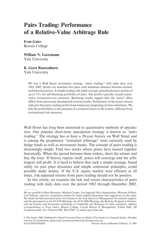
  • 8. most of the profits coming from the long end.3 We test long and short positions separately to see if this is driving our results. 2. Methodology Our implementation of pairs trading has two stages. We form pairs over a 12-month period (formation period) and trade them in the next 6-month period (trading period). Both 12 months and 6 months are chosen arbi- trarily and have remained our horizons since the beginning of the study. 2.1 Pairs formation In each pairs formation period, we screen out all stocks from the CRSP daily files that have one or more days with no trade. This serves to identify relatively liquid stocks as well as to facilitate pairs formation. Next, we construct a cumulative total returns index for each stock over the forma- tion period. We then choose a matching partner for each stock by finding the security that minimizes the sum of squared deviations between the two normalized price series. Pairs are thus formed by exhaustive matching in normalized daily ‘‘price’’ space, where price includes reinvested dividends. We use this approach because it best approximates the description of how traders themselves choose pairs. Interviews with pairs traders suggest that they try to find two stocks whose prices ‘‘move together.’’ In addition to ‘‘unrestricted’’ pairs, we will also present results by sector, where we restrict both stocks to belong to the same broad industry categories defined by Standard and Poors: Utilities, Transportation, Financial, and Industrials. Each stock is assigned to one of these four groups, based on the stock’s SIC code. The minimum-distance criterion is then used to match stocks within each of the groups. 2.2 Trading period Once we have paired up all liquid stocks in the formation period, we study the top 5 and 20 pairs with the smallest historical distance measure, in addition to the 20 pairs after the top 100 (pairs 101–120). This last set is valuable because most of the top pairs share certain characteristics, which will be described in detail below. On the day following the last day of the pairs formation period, we begin to trade according to a prespecified rule. Figure 1 illustrates the pairs trading strategy using two stocks, Kennecott and Uniroyal, in the six-month period starting in August of 1962. The top two lines represent the normalized price paths with dividends reinvested and the bottom line indicates the opening and closing of the strategy on a daily basis. It is clear why these two firms paired with each other. They generally tended to move together over the trading interval. 3 We thank an anonymous referee for this example. Pairs Trading 803
  • 9. Notice that the position first opens in the seventh trading day of the period and then remains open until day 36. Over that interval, the spread actually first increased significantly before convergence. The prices remain close during the period and cross frequently. The pair opens five times during the period, however not always in the same direction. Neither stock is the ‘‘leader.’’ In our example, convergence occurs in the final day of the period, although this is not always the case. We select trading rules based on the proposition that we open a long– short position when the pair prices have diverged by a certain amount and close the position when the prices have reverted. Following practice, we base our rules for opening and closing positions on a standard deviation metric. We open a position in a pair when prices diverge by more than two historical standard deviations, as estimated during the pairs forma- tion period. We unwind the position at the next crossing of the prices. If prices do not cross before the end of the trading interval, gains or losses are calculated at the end of the last trading day of the trading interval. If a stock in a pair is delisted from CRSP, we close the position in that pair, using the delisting return, or the last available price.4 We report the Figure 1 Daily normalized prices: Kennecott and Uniroyal (pair 5) Trading period August 1963–January 1964. 4 The profits are robust with respect to this delisting assumption. A potential problem arises if inaccurate and stale prices exaggerate the excess returns and bias the estimated return of a long position in a plummeting stock. To address this potential concern, we have reestimated our results under the extreme assumption that only a long stock experiences a –100% return when it is delisted. This zero-price extreme includes, among other things, the possibility of nontrading due to the lack of liquidity. Because selective loss on the long position always harms the pair profit, this extreme assumption biases the results against profitability. However, pairs trading remains profitable under this alternative: for example, the average monthly return on the top 20 pairs portfolio is 1.32% with a standard deviation of 1.9%. The Review of Financial Studies / v 19 n 3 2006 804
  • 10. payoffs by going one dollar short in the higher-priced stock and one dollar long in the lower-priced stock. 2.3 Excess return computation Because pairs may open and close at various points during the six-month trading period, the calculation of the excess return on a portfolio of pairs is a nontrivial issue. Pairs that open and converge during the trading interval will have positive cash flows. Because pairs can reopen after initial convergence, they can have multiple positive cash flows during the trading interval. Pairs that open but do not converge will only have cash flows on the last day of the trading interval when all positions are closed out. Therefore, the payoffs to pairs trading strategies are a set of positive cash flows that are randomly distributed throughout the trading period, and a set of cash flows at the end of the trading interval that can be either positive or negative. For each pair we can have multiple cash flows during the trading interval, or we may have none in the case when prices never diverge by more than two standard deviations during the trading interval. Because the trading gains and losses are computed over long–short positions of one dollar, the payoffs have the interpretation of excess returns. The excess return on a pair during a trading interval is computed as the reinvested payoffs during the trading interval.5 In parti- cular, the long and short portfolio positions are marked-to-market daily. The daily returns on the long and short positions are calculated as value- weighted returns in the following way, rP;t ¼ P iEP wi;tri;t P iEPwi;t ð2Þ wi;t ¼ wi;tÀ1ð1 þ ri;tÀ1Þ ¼ ð1 þ ri;1Þ Á Á Á ð1 þ ri;tÀ1Þ ð3Þ where r defines returns and w defines weights, and the daily returns are compounded to obtain monthly returns. This has the simple interpreta- tion of a buy-and-hold strategy. We consider two measures of excess return on a portfolio of pairs: the return on committed capital and the fully invested return, that is, the return on actual employed capital. The former scales the portfolio payoffs by the number of pairs that are selected for trading, the latter divides the payoffs by the number of pairs that open during the trading period. The former measure of excess return is clearly more conservative: if a pair does not trade for the whole of the trading period, we still include a dollar 5 This is a conservative approach to computing the excess return, because it implicitly assumes that all cash earns zero interest rate when not invested in an open pair. Because any cash flow during the trading interval is positive by construction, it ignores the fact that these cash flows are received early and understates the computed excess returns. Pairs Trading 805
  • 11. of committed capital as the cumulative return in our calculation of excess return. It takes into account the opportunity cost of hedge funds of having to commit capital to a strategy even if the strategy does not trade. To the extent that hedge funds are flexible in their sources and uses of funds, computing excess return relative to the actual capital employed may give a more realistic measure of the trading profits. We initiate the pairs strategy by trading the pairs at the beginning of every month in the sample period, with the exception of the first 12 months, which are needed to estimate pairs for the strategy starting in the first month. The result is a time series of overlapping six-month trading period excess returns. We correct for the correlation induced by overlap by averaging monthly returns across trading strategies that start one month apart as in Jegadeesh and Titman (1993). The resulting time series has the interpretation of the payoffs to a proprietary trading desk, which delegates the management of the six portfolios to six different traders whose formation and trading periods are staggered by one month. 3. Empirical Results 3.1 Strategy profits Table 1 summarizes the excess returns for the pairs portfolios that are unrestricted in the sense that the matching stocks do not necessarily belong to the same broad industry categories. In Section 3.5 we will consider sector-neutral pairs strategies. Panel A summarizes the excess returns of pairs strategies when positions are opened at the end of the day that prices diverge and closed at the end of the day of price convergence. The first row shows that a fully invested portfolio of the five best pairs earned an average excess monthly return of 1.31% (t-statistic = 8.84), and a portfolio of the 20 best pairs 1.44% per month (t = 11.56). Using the more conservative approach to computing excess returns, using com- mitted capital, gives excess returns of 0.78 and 0.81% per month, respec- tively. Either way, these excess returns are large in an economical and statistical sense and suggest that pairs trading is profitable. The remainder of Panel A provides information about the excess return distributions of pairs portfolios. There are diversification benefits from combining multiple pairs in a portfolio. As the number of pairs in a portfolio increases, the portfolio standard deviation falls. The diversifica- tion benefits are also apparent from the range of realized returns. Inter- estingly, as the number of pairs in the strategy increases, the minimum realized return increases, whereas the maximum realized excess return remains relatively stable. During the full sample period of 474 months, a portfolio of 20 pairs experienced 71 monthly periods with negative pay- offs, compared to 124 months for a portfolio of 5 pairs. The decrease in The Review of Financial Studies / v 19 n 3 2006 806
  • 12. the standard deviation and the increase of the lower end of the return distribution are also reflected in an increased skewness coefficient. Because pairs trading is in essence a contrarian investment strategy, the returns may be biased upward because of the bid-ask bounce [Jegadeesh (1990), Jegadeesh and Titman (1995), Conrad and Kaul (1989)]. In parti- cular, our strategy sells stocks that have done well relative to their match and buys those that have done poorly. Part of any observed price diver- gence is potentially due to price movements between bid and ask quotes: conditional on divergence, the winner’s price is more likely to be an ask quote and the loser’s price a bid quote. In Panel A we have used these same prices for the start of trading and our returns may be biased upward because of the fact that we are implicitly buying at bid quotes (losers) and selling at ask quotes (winners). The opposite is true at the second crossing Table 1 Excess returns of unrestricted pairs trading strategies Pairs portfolio Top 5 Top 20 101–120 All A. Excess return distribution (no waiting) Average excess return (fully invested) 0.01308 0.01436 0.01081 0.01104 Standard error (Newey-West) 0.00148 0.00124 0.00094 0.00099 t-Statistic 8.84 11.56 11.54 11.16 Excess return distribution Median 0.01194 0.01235 0.00955 0.00728 Standard deviation 0.02280 0.01688 0.01540 0.01670 Skewness 0.62 1.39 1.34 3.42 Kurtosis 7.81 10.54 10.30 25.25 Minimum –0.10573 –0.06629 –0.03857 –0.02721 Maximum 0.14716 0.13295 0.12684 0.17178 Observations with excess return < 0 26% 15% 21% 17% Average excess return on committed capital 0.00784 0.00805 0.00679 0.00614 B. Excess return distribution (one day waiting) Average monthly return (fully invested) 0.00745 0.00895 0.00795 0.00715 Standard error (Newey-West) 0.00119 0.00096 0.00085 0.00090 t-Statistic 6.26 9.29 9.40 7.92 Excess return distribution Median 0.00699 0.00690 0.00694 0.00411 Standard deviation 0.02101 0.01527 0.01438 0.01577 Skewness 0.34 1.45 0.98 3.32 Kurtosis 10.64 16.13 7.78 25.66 Minimum –0.12628 –0.08218 –0.04266 –0.02951 Maximum 0.14350 0.13490 0.10464 0.16325 Observations with excess return < 0 35% 23% 28% 32% Average excess return on committed capital 0.00463 0.00520 0.00503 0.00396 Summary statistics of the monthly excess returns on portfolios of pairs between July 1963 and December 2002 (474 observations). We trade according to the rule that opens a position in a pair at the end of the day that prices of the stocks in the pair diverge by two historical standard deviations (Panel A). The results in Panel B correspond to a strategy that delays the opening of the pairs position by one day. All pairs are ranked according to least distance in historical price space. The ‘‘top n’’ portfolios include the n pairs with least distance measures, and the portfolio ‘‘101–120’’ studies the 20 pairs after the top 100. The average number of pairs in the all-pair portfolio is 2057. The t-statistics are computed using Newey- West standard errors with six-lag correction. Absolute kurtosis is reported. Pairs Trading 807
  • 13. (convergence): part of the drop in the winner’s price can reflect a bid quote, and part of the rise of the loser’s price—an ask quote. To address this issue, Panel B of Table 1 provides the excess returns when we initiate positions in each pair on the day following the diver- gence and liquidate on the day following the crossing. The average excess returns on the fully invested portfolios and on committed capital drop by about 30–55 and 20–35 basis points (bp), respectively. Although the excess returns remain significantly positive, the drop in excess returns suggests that a nontrivial portion of the profits in Panel A may be due to bid–ask bounce. It is difficult to quantify which portion of the profit reduction is due to bid–ask bounce and which portion stems from true mean reversion in prices because of rapid market adjustment. Nonethe- less, this difference raises questions about the economic significance of our results when we include transaction costs. We will return to a detailed discussion of this issue in Section 3.3. Unless stated otherwise, the remain- der of the article will report results for pairs strategies that open (close) on the day following divergence (convergence). 3.2 Trading statistics and portfolio composition Table 2 summarizes the trading statistics and composition of the pairs portfolios. What are the characteristics of the stocks that are matched into pairs? How often does a typical pair trade? Because pairs trading is an active investment strategy, it is important to evaluate the profitability relative to the trading intensity of the portfolios. As mentioned before, we use a two standard deviation trigger to open a pairs position. The second line of panel A in Table 2 reports the average price deviation of the two standard deviation trigger. For the top five pairs, the position typically opens when prices have diverged by 4.76% or more. This is a relatively narrow gap in prices.6 The trigger spread increases with the number of pairs in the portfolio, because the standard deviation of the prices increases as the proximity of the securities in price space decreases. The next lines of Panel A also shows that on average almost all pairs open during the six-month trading period, and on average more than once. Of the top 5 pairs, on average 4.81 open during the trading period, and the average number of round trips per pair is 2.02. The average duration of an open position is 3.75 months. This indicates that pairs trading— implemented according to the particular rules we chose—is a medium- term investment strategy. Panel B of Table 2 describes the composition of the pairs in terms of market capitalization and industry membership. In terms of size, the average stock in the top 5 and top 20 pairs belongs to the second and 6 The optimal trigger point in terms of profitability may actually be much higher than two standard deviations, although we have not experimented to find out. The Review of Financial Studies / v 19 n 3 2006 808
  • 14. third deciles from the top; 74% of the stocks in the top 20 pairs belong to the top three size deciles using CRSP breakpoints, and 91% come from the top five size deciles. About two-thirds of the pairs combine stocks from different size deciles (i.e., ‘‘size mixed pairs’’), and the stocks in mixed pairs differ on average by a single decile. The remainder of Panel B gives a breakdown of the pairs by industry composition. On average, 71% of the stocks in the top 20 pairs are utility stocks, despite the fact that Utilities represent a fairly small proportion of the stocks in the whole sample. This is not surprising perhaps because utility stocks tend to have lower volatility and tend to be correlated with interest rate innovations. The strategy does not always match stocks within sectors. The percentage of mixed sector pairs ranges from 20% for the top five pairs to 44% for pairs 101–120. Given the predominance of utilities among the top pairs, it is fair to ask whether the profitability of pairs trading profitability is limited to the utility sector, or whether pairs strategies are also profitable in other sectors of the market. We address this question in Section 3.5. Table 2 Trading statistics and composition of pairs portfolios Pairs portfolio Top 5 Top 20 101–120 All A. Trading statistics Average price deviation trigger for opening pairs 0.04758 0.05284 0.07560 0.16888 Average number of pairs traded per six-month period 4.81 19.30 19.41 1944.22 Average number of round-trip trades per pair 2.02 1.96 1.78 1.62 Standard deviation of number of round trips per pair 0.62 0.40 0.27 0.16 Average time pairs are open in months 3.75 3.76 3.98 3.97 Standard deviation of time open, per pair, in months 0.80 0.45 0.38 0.17 B. Pairs portfolio composition Average size decile of stocks 2.54 2.71 3.41 4.57 Average weight of stocks in top three size deciles 0.78 0.74 0.58 0.40 Average weight of stocks in top five size deciles 0.91 0.91 0.79 0.62 Average weight of pairs from different deciles 0.66 0.69 0.75 0.82 Average decile difference for mixed pairs 0.97 0.97 0.97 0.98 Average sector weights Utilities 0.72 0.71 0.32 0.08 Transportation 0.02 0.02 0.02 0.03 Financials 0.11 0.13 0.26 0.16 Industrials 0.15 0.14 0.40 0.73 Mixed sector pairs 0.20 0.22 0.44 0.33 Trading statistics and composition of portfolios of pairs portfolios between July 1963 and December 2002 (474 months). Pairs are formed over a 12-month period according to a minimum-distance criterion and then traded over the subsequent 6-month period. We trade according to the rule that opens a position in a pair on the day following the day on which the prices of the stocks in the pair diverge by two historical standard deviations. The ‘‘top n’’ portfolios include the n pairs with least distance measures, and the portfolio ‘‘101–120’’ includes the 20 pairs after the top 100. Panel A summarizes the trading characteristics of a pairs strategy. Pairs are opened when prices diverge by two standard deviations. Average deviation to trigger opening of pair is the cross-sectional average of two standard deviations of the pair prices difference. Panel B contains information about the size and industry membership of the stocks in the various pairs portfolios. Pairs Trading 809
  • 15. 3.3 Transaction costs Table 1 summarizes that the average monthly excess return of unrest- ricted pairs strategies falls from 1.44%, for the top 20 portfolio, to 0.90% per month if we postpone the trades to the day following the crossing. This drop in the excess returns implies an estimate of the average bid-ask spread and hence the transaction costs of trading in the sample. Although actual transaction costs may be different, it is informative to know whether the trading profits are large enough to survive this estimate of transaction costs. Suppose the extreme case where the prices of the winner at the first crossing (divergence) are ask prices and the loser are bid prices. If the next day prices are equally likely to be at bid or ask, then delaying trades by one day will reduce the excess returns on average by half the sum of the spreads of the winner and the loser. If at the second crossing (con- vergence) of the pairs the winner is trading at the bid and the loser at the ask, waiting one day will reduce the excess returns on average again by one-half of the sum of the bid–ask spreads of both stocks. In this extreme case, waiting a day before trading reduces the return on each pair by the round-trip transaction costs in that pair. Because we trade each pair on average two times during the six-month trading interval, the drop in the excess returns of 324 bp per six months by waiting one day reflects the cost of two round trips, which implies a transaction cost of 162 bp per pair per round trip. This may be interpreted as an estimated effective spread of 81 bp. The effective spread for the all- pair portfolio is 70 bp. This indirect estimate is higher than the transac- tion costs reported by Peterson and Fialkowski (1994), who find that the average effective spread for stocks in the CRSP database in 1991 was 37 bp, and is consistent with the trading costs estimated by Keim and Madhavan (1997). Because 91% of the stocks in the top 20 pairs belong to the top five deciles of CRSP stocks, it is possible that the effective spread is even lower that 37 bp. Do our trading strategies survive these transaction costs? The profits on our trading strategies in Table 1 range from 437 to 549 bp over a six- month period. If the prices used to compute these excess returns are equally likely to be at bid or ask, which seems a reasonable assumption, we have to correct these excess returns to reflect that in practice we buy at the ask and sell at the bid prices. In other words, we have to subtract the round-trip trading costs to get an estimate of the profits after transaction costs. Our conservative estimate of transaction costs of 162 bp times two round trips per pair results in an estimate of 324 bp transaction cost per pair per six-month period. This gives average net profits ranging from 113 to 225 bp over each six-month period. Comparing these profits to the reported standard errors, we conclude that they are both economically and statistically significant. The Review of Financial Studies / v 19 n 3 2006 810
  • 16. Further analysis is required to get more precise estimates of influence of transaction costs of pairs trading strategies. An important question in this context is whether the trading rule that we have used to open and close pairs can be expected to generate economically significant profits even if pairs trading works perfectly. Because we use a measure of historical standard deviation to trigger the opening of pairs, and because this estimated standard deviation is the smallest among all pairs, it is likely to underestimate the true standard deviation of a pair. As a consequence, we may simply be opening pairs ‘‘too soon’’ and at a point that we cannot expect it to compensate for transaction costs even if the pair subsequently converges. Results that are not reported here suggest that this is indeed the case for some of our pairs. There is a second reason why our trading strategies require ‘‘too much’’ trading. We open pairs at any point during the trading period when the normalized prices diverge by two standard deviations. This is not a sensible rule toward the end of a trading interval. For example, suppose that a divergence occurs at the next to last day of the trading interval. The convergence has to be substantial to overcome the transaction cost that will be incurred when we close out the position on the next day (the last day of the trading interval). Unreported results suggest that this is also an important source of excess trading. 3.4 Pairs trading by industry group The pairs formation process thus far has been entirely mechanical. A computer stock has the opportunity to match with a steel firm and a utility with a bank stock. This does not mean that these matches are likely. As summarized in Table 2, the fraction of mixed pairs is typically well below 50%. Common factor exposures of stocks in the same industry will make it more likely to find a match within the same sector. Also, firms that are in industries where cross-sectional differences in factor exposures are small or return variances are low are more likely to end up among the top ranking of pairs. For this reason it is perhaps not surprising that many of the top pairs match two utilities. Are the profits to pairs trading consistent across sectors? We examine the returns on pairs trading where stocks are matched only within the four large sector groupings used by Standard and Poor’s: Utilities, Transportation, Finan- cials, and Industrials. The results are summarized in Table 3. As in Table 1, the pairs are traded with a one-day delay before opening and closing a position to minimize the effect of the bid–ask bounce on trading. The monthly excess returns for the top 20 pairs are the largest in the Utilities sector, with 1.08% (Newey-West t = 10.26). The profits for the other industry groups are somewhat lower, but all statistically significant, with the average Transportation, Financials, and Industrials top 20 pairs earning 0.58% (Newey-West t = 4.26), 0.78% (Newey-West Pairs Trading 811
  • 17. t = 7.60), and 0.61% (Newey-West t = 6.93), respectively, over a one-month period. Table 3 also gives a more detailed picture of the return distributions and trading characteristics of the pairs trading strategies by sector. It shows that Table 3 Industry sector pairs trading Portfolio Top 5 Top 20 20 after 100 All A. Utilities Mean excess return 0.00905 0.01084 0.009256 0.01036 t-Statistic (Newey-West) 7.37 10.26 6.11 10.51 Median 0.00829 0.00938 0.00665 0.00969 Standard deviation 0.02154 0.01645 0.02640 0.01472 Skewness 0.44 0.76 0.66 1.39 Kurtosis 13.67 12.38 5.52 12.74 Minimum 70.12347 70.08750 70.07868 70.03519 Maximum 0.16563 0.12730 0.12133 0.12878 Observations with excess return < 0 28% 19% 35% 18% B. Transportation Mean excess return 0.00497 0.00577 0.00440 t-Statistic (Newey-West) 2.98 4.26 3.07 Median 0.00594 0.00547 0.00339 Standard deviation 0.03892 0.02942 0.02871 Skewness 70.50 70.11 0.53 Kurtosis 4.98 5.00 5.89 Minimum 70.19570 70.12467 70.12526 Maximum 0.10961 0.11099 0.13560 Observations with excess return < 0 44% 42% 44% C. Financials Mean excess return 0.00678 0.00775 0.00854 0.00726 t-Statistic (Newey-West) 4.79 7.60 7.12 7.62 Median 0.00557 0.00615 0.00660 0.00511 Standard deviation 0.02598 0.01792 0.02358 0.01808 Skewness 0.81 0.61 1.98 2.64 Kurtosis 6.37 6.48 18.27 21.21 Minimum 70.081988 70.07810 70.100477 70.04452 Maximum 0.149291 0.10638 0.195797 0.17211 Observations with excess return < 0 40% 33% 32% 34% D. Industrial Mean excess return 0.00490 0.00607 0.00664 0.00715 t-Statistic (Newey-West) 4.11 6.93 6.80 7.52 Median 0.00292 0.00547 0.00550 0.00397 Standard deviation 0.02361 0.01601 0.01825 0.01672 Skewness 0.40 0.43 0.94 2.97 Kurtosis 4.94 4.75 7.65 20.95 Minimum 70.10016 70.04786 70.05412 70.03431 Maximum 0.10546 0.08022 0.11619 0.16072 Observations with excess return < 0 42% 36% 35% 34% Summary statistics for the excess monthly return distributions for pairs trading portfolios by sector. We trade according to the ‘‘wait one day’’ rule described in the text. The average number of stocks in the industry groups are as follows: 156 Utilities, 61 Transportation, 371 Financials, and 1729 Industrials. There is no ‘‘20 after 100’’ portfolio for the Transportation industry group. The t-statistic of the mean is computed using Newey-West standard errors with six lags. The Review of Financial Studies / v 19 n 3 2006 812
  • 18. the excess return distributions of the sector pairs portfolios are generally skewed right and exhibit positive excess kurtosis relative to a normal distribution. The conclusion from these tables is that pairs trading is profit- able in every broad sector category, and not limited to a particular sector. 3.5 The risk characteristics of pairs trading strategies To provide further perspective on the risk of pairs trading, Table 4 compares the risk-premium of pairs trading to the market premium (S&P 500) and reports the risk-adjusted returns to pairs trading using two different models for measuring risk. Table 5 summarizes value-at-risk (VAR) measures for pairs portfolios. The top part of Table 4 compares the excess return to pairs trading to the excess return on the S&P 500. Between 1963 and 2002, the average excess return to pairs trading has been about twice as large as the excess return of the S&P 500, with only one-half to one-third of the risk as measured by standard deviation. As a result, the Sharpe Ratios of pairs trading are between four and six times larger than the Sharpe Ratio of the market. Goetzmann et al. (2002) show that Sharpe Ratios can be mis- leading when return distributions have negative skewness. This is unlikely to be a concern for our study, because our Table 1 showed that the returns to pairs portfolios are positively skewed, which—if anything— would bias our Sharpe Ratios downward. To explore the systematic risk exposure of the pairs portfolios, we regress their monthly excess returns on the three factors of Fama and French (1996), augmented by two additional factors. The motivation for the additional factors is that pairs strategies invest based on the relative strength of individual stocks. It is therefore possible that pairs trading simply exploits patterns in returns that are known to earn significant profits. For example, Jegadeesh (1990) and Lehmann (1990) show that reversal strategies that select stocks based on prior one-month return earn positive abnormal returns. We control for this possibility by constructing a short-term reversal factor measured as the excess return of stocks in the top three deciles of prior-month return minus the return on stocks in the bottom three deciles.7 If pairs strategies sell short-term winners and buy short-term losers, we expect the exposures of pairs portfolios to be positive to the reversal factor. The second additional factor controls for exposure to medium-term return continuation [Jegadeesh and Titman (1993)]. To the extent that pairs trading sells medium-term winners and buys medium-term losers, the pairs excess returns will be negatively correlated with momentum. To examine this possibility, we include a 7 The construction is similar to Carhart’s (1997) momentum factor, but the performance-sorting horizon here is one month. Pairs Trading 813
  • 19. Table 4 Systematic risk of pairs trading strategies Top 5 Top 20 20 after top 100 All Equity premium ‘‘Wait one day’’ portfolio performance Mean excess return 0.00745 0.00895 0.00795 0.00715 0.00410 Standard deviation 0.02101 0.01527 0.01438 0.01577 0.04509 Sharpe Ratio 0.35 0.59 0.55 0.45 0.09 Monthly serial correlation 0.14 0.24 0.19 0.12 0.05 Factor model: Fama–French, Momentum, Reversal Intercept 0.00545 (3.81) 0.00764 (7.08) 0.00714 (8.66) 0.00512 (5.30) Market 70.06661 (–1.03) 70.03155 (–0.64) 70.07697 (–1.77) 70.14520 (–3.10) SMB 70.04233 (–0.71) 0.00111 (0.02) 70.02333 (–0.50) 70.07079 (–1.66) HML 0.05740 (1.37) 0.04514 (1.45) 70.01724 (–0.59) 70.05403 (–1.82) Momentum 70.02804 (–0.94) 70.04817 (–2.45) 70.10312 (–5.83) 70.18077 (–8.50) Reversal 0.10192 (1.50) 0.07237 (1.27) 0.09459 (2.24) 0.20077 (4.34) R2 0.05 0.09 0.18 0.54 Factor model: Ibbotson factors Intercept 0.00716 (6.32) 0.00857 (9.25) 0.00766 (9.39) 0.00651 (7.77) Market 70.00182 (–0.07) 0.01377 (0.74) 0.01642 (0.90) 0.06466 (1.98) Small stock premium 0.04120 (1.32) 0.05227 (2.22) 0.03646 (1.66) 0.07608 (1.93) Bond default premium 0.14593 (1.11) 0.15989 (1.38) 0.16811 (1.81) 0.30571 (2.82) Bond horizon premium 0.07997 (1.55) 0.06818 (1.64) 0.04034 (1.04) 0.03422 (0.77) R2 0.02 0.05 0.04 0.15 Monthly risk exposures for portfolios of pairs formed and traded according to the ‘‘wait one day’’ rule discussed in the text, over the period between June 1963 and December 2002. The five actors are the three Fama–French factors, Carhart’s Momentum factor, and the Reversal factor discussed in the text. Returns for the portfolios are in excess of the riskless rate. S&P 500 returns are calculated in excess of Treasury bill returns. The Ibbotson factors are from the Ibbotson EnCorrr analyzer: The U.S. Small stock premium is the monthly geometric difference between small-company stock total returns and large-company stock total returns. U.S. bond default premium is the monthly geometric difference between total return to long-term corporate bonds and long-term government bonds. The U.S. bond horizon premium is the monthly geometric difference between investing in long-term government bonds and U.S. Treasury bills. The t-statistics are in parentheses next to the coefficients and are computed using Newey-West standard errors with six lags. TheReviewofFinancialStudies/v19n32006 814
  • 20. momentum factor in our risk model that is constructed along the lines of Carhart (1997). Table 4 demonstrates that only a small portion of the excess returns of pairs trading can be attributed to their exposures to the five risk factors. The intercepts of the regressions show that risk-adjusted returns are significantly positive and lower than the raw excess returns by about 10–20 bp per month. Because pairs strategies are market-neutral, the exposures to the market are small and with one exception insignificant. Exposures to the other two Fama–French factors, the difference between small and big stocks (SMB) and the difference between value and growth stocks (HML), are not significant and the point estimates alternate in sign. The exposures to momentum and reversals have the predicted signs, and more than half are statistically significant. As can be expected, some of the winner stocks that a pairs strategy shorts are short-term winners, whereas others are medium-term winners. Similarly, the losers are evenly divided between short-term and medium-term losers. Overall the expo- sures are not large enough to explain the average returns to pairs trading. Table 5 Value at risk (VAR) of pairs trading Top 5 Top 20 20 after 100 All A. Monthly var Mean excess return 0.00745 0.00895 0.00795 0.00715 Standard deviation 0.02101 0.01527 0.01438 0.01577 Serial correlation 0.14 0.24 0.19 0.12 VAR 1% 70.04320 70.01943 70.02236 70.01994 5% 70.02142 70.01002 70.01293 70.00877 10% 70.01516 70.00577 70.00756 70.00614 25% 70.00460 0.00054 70.00145 70.00146 Probability of return below 0 0.35 0.23 0.28 0.32 Minimum historical observation 70.12628 70.08218 70.04266 70.02951 B. Daily var Mean excess return 0.00033 0.00040 0.00035 0.00027 Standard deviation 0.00492 0.00296 0.00277 0.00169 Serial correlation 70.12 70.06 0.00 0.35 VAR 1% 70.01236 70.00647 70.00653 70.00327 5% 70.00710 70.00398 70.00400 70.00202 10% 70.00504 70.00293 70.00288 70.00149 25% 70.00239 70.00133 70.00130 70.00071 Probability of return below 0 0.47 0.44 0.45 0.46 Minimum historical observation 70.10079 70.06723 70.01987 70.01069 Monthly and daily VAR percentiles of pairs trading strategies between July 1963 and December 2002 (474 months). Pairs are formed over a 12-month period according to a minimum-distance criterion, and then traded over the subsequent 6-month period. We trade according to the rule that opens a position in a pair on the day following the day on which the prices of the stocks in the pair diverge by two historical standard deviations. The ‘‘top n’’ portfolios include the n pairs with least distance measures, and the portfolio ‘‘101–120’’ includes the 20 pairs after the top 100. The average number of pairs in the all-pair portfolio is 2057. Pairs Trading 815
  • 21. The significance of the risk-adjusted returns indicates that pairs trading is fundamentally different from simple contrarian strategies based on rever- sion [Jegadeesh (1990) and Lehmann (1990)]. The next sections provide further evidence to support this view. The bottom of Table 4 reports the results of regressing the pairs returns on an alternative set of risk factors suggested by Ibbotson: the excess return on the S&P 500, the U.S. small stock premium, the U.S. bond default premium, and the U.S. bond horizon premium. Although the risk exposures are generally not significant, the signs of coefficients are positive across all portfolios. Thus, when corporate bonds increase in price relative to government bonds, the pairs portfolios make money. There are a range of possible explanations for this pattern. Relatively cheaper borrowing rates by arbitrageurs may force stock prices closer to equilibrium values, or common factors affecting convergence in both stock and bond markets may be responsible. The portfolios also appear to be sensitive to shifts in the yield curve, that is, when long-term spreads decrease, pairs trading is more profitable. At first glance, the sensitivity to term-structure measures may be explained by the presence of interest rate sensitive Utility stocks in many of the top pairs. However, interest rate movements also seem to matter for the more broadly diversified pairs portfolios. In sum, the pairs portfolios seem to have low exposure to various sources of systematic risk. The R-squared of most regressions is low, indicating that the portfolios are nearly factor-neutral. This may be expected because they are constructed in a way that should essentially match up economic substitutes. Table 5 reports both monthly and daily VAR measures to summarize the quantiles of the empirical distributions of the pairs’ excess returns. Panel A shows that the worst monthly loss over the almost 40-year sample period was 12.6% for the top five pairs portfolio, and 8.2% for the top 20 portfolio. On average, only once in every hundred months did these portfolios lose more than 4.32 and 1.94%, respectively. Panel B shows that on its worst day, the top five portfolio recorded a 10.08% loss, compared to a 6.72% loss of the top 20 portfolio. On average, only once every hundred days did these portfolios lose more than 1.24% and 0.65%, respectively. The VAR is useful because it provides a gauge to the potential leverage that could be applied to these strategies. A five-to-one leverage ratio applied to the top five pairs would appear to have been adequate to cover the worst monthly loss in the 40-year period. Although the lessons of recent history have taught us not to rely too heavily on historical VAR measures for gauging capital needs for exploiting convergence strategies, the pairs portfolios seem to be exposed to relatively little risk. Figure 2 shows the monthly performance of the top 20 pairs, based on the next-day trading rule. Pairs trading was very profitable in the 1970s The Review of Financial Studies / v 19 n 3 2006 816
  • 22. and 1980s, and then had a span of more modest performance, when the returns were sometimes negative. Figure 3 compares the cumulative excess returns of the top 20 one-day-waiting strategy with the cumulative excess returns of investment in the S&P 500 index. The smooth index of the pairs trading portfolio contrasts dramatically with the volatility of the Figure 2 Monthly excess returns of top 20 pairs portfolio May 1963–December 2002. Figure 3 Cumulative excess return of top 20 pairs and S&P 500 May 1963–December 2002. Pairs Trading 817
  • 23. stock market. Pairs trading performed well over difficult times for U.S. stocks. When the U.S. stock market suffered a dramatic real decline from 1969 through 1980, the pairs strategy experienced some of its best perfor- mance. By contrast, in the mid-1990s the market performed exceptionally well, but pairs trading profits were relatively flat. Perhaps after its dis- covery in the early 1980s by Tartaglia and others, competition decreased opportunity. On the other hand, pairs trading might simply be more profitable in times when the stock market performs poorly. Two additional explanations may account for the temporal variation in profitability. The first is the long-term trend in transaction costs over the history of our sample. The early part of the analysis represents a period with high fixed commissions. These frictions might have prevented the rapid convergence of relative prices. The secular decrease in transaction costs may have attracted more relative-value equity arbitrage. This is becoming increasingly so with the introduction of more sophisticated trading technologies and networks. The second explanation may be the rise in hedge funds in the period since 1989. The TASS hedge fund database reports that hedge fund assets rose from $4 billion in 1977 to $137 billion in 2000, with the most dramatic growth after 1992. Although this database does not capture proprietary trading operations of invest- ment banks, it does suggest that risk arbitrage activities have grown significantly in the last decade of our sample period. Of the $137 billion in hedge fund assets in 2000, $119 billion employed ‘‘Market Neutral’’ ‘‘Relative Value’’ or ‘‘Arbitrage’’ strategies, all of which may potentially impact pairs trading operations. Thus, it is possible that lower transaction costs and large inflows of investment capital to relative-value arbitrage have together decreased the rate of return on pairs trading, at least in the simple form we test in this article. In Section 3.8, we will revisit this issue and show that in contrast to the raw returns the risk-adjusted return to pairs trading has been relatively stable over time. 3.6 Pairs trading and contrarian investment Because pairs trading bets on price reversals, it is an example of a contra- rian investment strategy. The results of Table 4 showed that the returns to pairs are positively correlated with—but not explained by—short-term reversals documented by Lehmann (1990) and Jegadeesh (1990). In this section we further explore whether our pairs trading strategies are merely a disguised way of exploiting these previously documented negative auto- correlations. In particular, we conduct a bootstrap where we compare the performance of our pairs to random pairs. The starting point of the bootstrap is the set of historical dates on which the various pairs open. In each bootstrap we replace the actual stocks with two random securities with similar prior one-month returns as the stocks in the actual pair. Similarity is defined as coming from the same decile of previous month’s The Review of Financial Studies / v 19 n 3 2006 818
  • 24. performance. The difference between the actual and the simulated pairs returns provides an indication of the portion of our pairs return that is not due to reversion. We bootstrapped the entire set of trading dates 200 times. The results are summarized in Table 6. On average we find that the returns on the bootstrapped pairs are well below the true pairs returns. In fact, the excess returns to the simulated pairs are slightly negative, and the standard deviations of the returns are large relative to the true pairs, which is a reflection of the fact that the simulated pairs are poorly matched. The conclusion from the simulations confirms the conclusion from the factor regressions that the pairs strategy does not merely reflect one-month mean reversion. In addition, in the next section, we will show that the long and short portfolios that make up a pair do not provide equal contributions to the profitability of the strategy. These three find- ings combined strongly suggest that our pairs trading strategy seems to capture temporal variation in returns that is different from simple mean reversion. 3.7 Risk and return of the long and short positions There are at least three reasons to separately examine the returns to the long and short portfolios that make up a pairs position. First, the Table 6 Returns to random pairs sorted on prior one-month return Portfolio Top 5 Top 20 Top 100–120 All 120 A. No waiting Fully invested Mean excess return 70.00137 70.00111 70.00105 70.00113 Standard deviation 0.05521 0.02295 0.02264 0.01200 Median 70.00192 70.00153 70.00156 70.00162 Committed capital Mean excess return 70.00083 70.00077 70.00089 70.00091 Standard deviation 0.02635 0.01358 0.01443 0.00760 Median 70.00123 70.00100 70.00123 70.00122 B. Wait one day Fully invested Mean excess return 70.00177 70.00004 70.00154 70.00156 Standard deviation 0.05966 0.05310 0.02404 0.01213 Median 70.00241 70.00172 70.00206 70.00201 Committed capital Mean excess return 70.00103 70.00094 70.00112 70.00112 Standard deviation 0.02811 0.01363 0.01449 0.00761 Median 70.00152 70.00118 70.00148 70.00139 Bootstrap of random pairs traded according to the rule that opens a position in a random pair when the stocks in the true pair diverge by two historical standard deviations and closes the position after the next crossing of prices. The random stocks are selected within the same last-month performance decile on the day the position is opened. The top panel gives summary statistics of the monthly excess returns on value- weighted portfolios of n pairs of stocks where the position is opened immediately. The last column is a portfolio of all 120 top pairs. The bottom panel summarizes the performance with one day waiting before the position is opened. The statistics are computed over 200 replications of the bootstrapped sample. Pairs Trading 819
  • 25. separate returns provide further insight into the question of mean rever- sion. If pairs trading simply exploits mean reversion, one would expect the abnormal returns to the long and short positions to be equal because the opening of a pair is equally likely to be triggered by either stock. Second, if the excess returns are predominantly driven by the short position, it becomes important to examine whether short-sale considera- tions might prevent arbitrageurs from competing away the profits. Finally, the risk exposures of the two portfolios can provide further clues to the reason for the profitability of pairs—for example, the possi- bility that the long and short portfolios have different exposures to common nonstationary risk factors such as bankruptcy risk.8 The returns and the risk exposures of the component portfolios are summarized in Table 7. The table demonstrates that much of the pairs risk-adjusted excess return comes from the short portfolio, which contains the stocks that have increased in value relative to their counterparts prior to opening of the pair. By contrast, the alphas of the long portfolio containing the stocks that decreased in value relative to their counterparts are smaller, and insignificantly different from zero for the top 5 and top 20 portfolios. The asymmetry of the results provides further evidence that the returns to pairs are not due to simple one-month mean reversion. And because much of the abnormal return comes from the short position, which experienced an increase in relative value prior to opening, it is unlikely that the returns are driven by a reward for unrealized bankruptcy risk. The robustness of our results to the cost of short sales will be discussed in Section 3.9. 3.8 Subperiod analysis and the presence of a dormant risk factor Table 8 summarizes the profitability of pairs trading when we split the sample period at the end of 1988. A comparison between the two top halves of the two panels shows a drop in the raw excess returns to pairs trading. For example, the excess return of the top 20 strategy drops from 118 bp per month to about 38 bp per month. Has increased hedge fund activity arbitraged away the anomalous behavior of pairs since the pre-1989 per- iod? Inspection of the risk-adjusted returns shows that this is not the case: the average risk-adjusted return of the top 20 portfolio drops by about one- third from 67 to 42 bp per month, but remains significantly positive in both subperiods (t = 4.41 and 3.77, respectively). Changes in the factor expo- sures and factor volatilities can explain only part of the lower returns in the early part of the sample, but not the risk-adjusted returns to pairs trading. Are the positive risk-adjusted returns to pairs trading a general failure of our risk model? In other words, are there reasons to believe that the 8 We thank a referee for suggesting this explanation. The Review of Financial Studies / v 19 n 3 2006 820
  • 26. Table 7 Returns to long and short components of pairs Top 5 Top 20 20 after top 100 All Portfolio Long Short Long Short Long Short Long Short Portfolio performance Mean monthly return 0.01245 0.00501 0.01330 0.00435 0.01458 0.00663 0.01623 0.00908 Standard error (Newey-West) 0.00183 0.00177 0.00179 0.00174 0.00170 0.00165 0.00254 0.00231 Standard deviation 0.03875 0.03259 0.03653 0.03161 0.03437 0.03146 0.05157 0.04601 Monthly serial correlation 0.06 0.11 0.09 0.12 0.13 0.12 0.17 0.16 Regression on Market, SMB, HML, Momentum, and Reversal factors Intercept 0.00103 70.00442 0.00243 70.00521 0.00287 70.00426 70.00101 70.00613 t-Statistic 0.47 72.74 1.27 73.35 2.85 74.26 71.32 75.22 U.S. equity risk-premium 0.37415 0.44075 0.47617 0.50772 0.48520 0.56217 0.58571 0.73091 t-Statistic 4.60 6.19 6.68 8.44 10.23 9.74 14.99 12.13 SMB 70.16764 70.12532 70.06506 70.06616 0.01120 0.03453 0.22192 0.29271 t-Statistic 71.74 72.00 70.80 71.22 0.27 0.95 3.45 3.15 HML 0.48401 0.42661 0.52539 0.48025 0.39451 0.41175 0.25732 0.31134 t-Statistic 7.12 6.92 9.36 9.47 9.76 11.54 7.49 8.11 Momentum 70.05430 70.02625 70.04456 0.00361 70.10901 70.00589 70.08832 0.09245 t-Statistic 71.48 70.65 71.21 0.10 73.53 70.21 73.53 2.81 Reversal 0.15854 0.05662 0.09601 0.02365 0.17288 0.07830 0.39208 0.19131 t-Statistic 1.83 1.13 1.26 0.55 4.33 1.90 10.44 2.98 R2 0.39 0.41 0.48 0.49 0.78 0.75 0.97 0.93 Monthly risk profile for the long and short positions of the pairs portfolios formed and traded according to the ‘‘wait one day’’ rule discussed in the text. The returns in the bottom half of the table are in excess of the 30-day Treasury bill returns. The risk adjustment includes the Fama–French factors, as well as Momentum and the Reversal factors discussed in the text. The t-statistics are computed using Newey-West standard errors with six lags. Absolute kurtosis is reported. PairsTrading 821
  • 27. risk-adjusted pairs returns are a compensation for an omitted (latent) risk factor? Inspection of the correlation between disjoint pairs portfolios provides some support for this view. Moreover, this latent risk factor seems to have been relatively dormant over the second half of our sample, which can account for the lower recent profitability of pairs trading. The full-sample correlation between the excess returns of the top 20 and the 100–120 pairs portfolios is 0.48. Because there is no overlap between the positions of these portfolios, the correlation indicates the presence of a Table 8 Subperiod analysis Portfolio Top 5 Top 20 20 after top 100 All Factor SD A. Pre-1989 ‘‘Wait one day’’ portfolio performance Mean excess return 0.01034 0.01181 0.01052 0.00992 Standard deviation 0.02259 0.01689 0.01527 0.01651 Regression on Fama–French factors Intercept 0.00353 0.00670 0.00710 0.00446 t-Statistic 1.72 4.41 6.54 4.19 U.S. equity risk-premium 70.43395 70.31200 70.28946 70.43429 0.04580 t-Statistic 74.29 73.57 73.80 77.26 SMB: small minus big 70.44181 70.33193 70.27508 70.40184 0.02923 t-Statistic 73.75 72.86 72.86 75.76 HML: high minus low book to market 0.03568 0.03162 70.06840 70.06983 0.02597 t-Statistic 0.64 0.73 71.84 71.97 Momentum 0.01291 70.01630 70.07689 70.15848 0.03506 t-Statistic 0.29 70.50 72.92 75.01 Reversal 0.43575 0.33274 0.28765 0.45222 0.07228 t-Statistic 4.44 3.62 4.05 7.98 R2 0.19 0.23 0.26 0.70 B. Post-1988 ‘‘Wait one day’’ portfolio performance Mean excess return 0.00217 0.00375 0.00327 0.00212 Standard deviation 0.01660 0.00987 0.01121 0.01295 Regression on Fama–French factors Intercept 0.00337 0.00417 0.00363 70.00065 t-Statistic 2.12 3.77 3.01 70.56 U.S. equity risk-premium 0.07339 0.04804 0.00241 70.06958 0.04390 t-Statistic 1.68 1.81 0.06 72.43 SMB: small minus big 70.00400 0.02888 0.02332 70.06063 0.03856 t-Statistic 70.10 1.32 0.69 72.83 HML: high minus low book to market 0.03441 0.01412 0.01830 70.08202 0.03641 t-Statistic 0.61 0.45 0.50 72.65 Momentum 70.00424 70.02266 70.08840 70.12670 0.04926 t-Statistic 70.13 71.29 74.17 77.59 Reversal 70.06259 70.01727 0.02404 0.18808 0.04448 t-Statistic 71.76 70.67 0.54 5.56 R2 0.02 0.04 0.19 0.64 Monthly risk profile for portfolios of pairs formed and traded according to the ‘‘wait one day’’ rule discussed in the text, over the two subperiods between July 1963 and December 1988 (Panel A) and between January 1989 and December 2002 (Panel B). The ‘‘top n’’ portfolios include the n pairs with least distance measures, and the portfolio ‘‘20 after top 100’’ includes the 20 pairs after the top 100 pairs. The average number of pairs in the all-pair portfolio is 2057. The t-statistics are computed using Newey-West correction with six lags for the standard errors. The Review of Financial Studies / v 19 n 3 2006 822
  • 28. common factor to the returns. Moreover, the correlation is 0.51 over the profitable pre-1988 period but much lower (0.18) over the lower excess return post-1988 period. These correlations are not driven by the 5 ‘‘systematic’’ risk factors we considered, because the correlations of the residuals from the factor regressions are very similar to the raw correlations. In particular, the correlation between the top 20 Fama–French-Momentum-Reversal (FFMR) residuals and the top 100–120 FFMR residuals is 0.41. The respec- tive subperiod FFMR correlations are 0.42 and 0.20. This is further illu- strated in Figure 4, which shows that the rolling 24-month correlation between the two portfolios was especially high during the pre-1989 period. These results suggest that there is common component to the profits of pairs portfolios that is not captured by our conventional measures of sys- tematic risk. The common component was stronger during the first half of our sample, which is consistent with higher profits (abnormal returns) than in the second half of our sample when the factor was more dormant. These results are consistent with the view that the abnormal returns documented in this article are indeed a compensation for risk, in particular the reward to arbitrageurs for enforcing the ‘‘Law of One Price.’’ 3.9 Robustness to short-selling costs Having identified and back-tested a filter rule, and subjected it to a range of controls for risk, the question of the nature of pairs profits remains. Why do prices of close economic substitutes diverge and converge? The Figure 4 Top 20 pairs and 101–120 pairs portfolios Rolling 24-month correlation of five-factor risk-adjusted excess returns. Pairs Trading 823
  • 29. convergence is easier to understand than the divergence, given the natural arbitrage motivation and the documented existence of relative-value arbi- trageurs in the U.S. equity market. However, this does not explain why prices drift away from parity in the first place. One possible explanation is that prices diverge on random liquidity shocks that cannot be exploited by professional arbitrageurs because of short-selling costs.9 First, there are explicit short-selling costs in the form of specials. Second, D’Avolio (2002) argues that short recalls are potentially costly because they may deprive arbitrageurs of their profits. This opportunity cost is reinforced by D’Avolio’s findings that short recalls are more common as the price declines. For example, if the short stock is recalled when it starts to converge downward, then the pairs position is forced to close prematurely and the arbitrageur does not capture the profit from the pair convergence. We perform two tests for robustness of the profits that corresponds to these two types of short-selling costs. The first test is motivated by the findings of D’Avolio (2002) and Geczy et al. (2002) that specials have minimal effect of large stocks. Correspondingly, we test for robustness of profits by trading pairs that are formed using only stocks in the top three size deciles.10 The results, given in Panel A of Table 9, can be directly compared to those in Panel B of Table 1. The comparison shows that the profits of the top 20 strategy drop by about 2 bp per month, but increase for the top five portfolios. Overall, the profits change little and remain highly significant. This shows that the pairs trading profits are not driven by illiquid stocks that are likely to be on special. The second test is motivated by the evidence in Chen et al. (2002) and D’Avolio (2002) that short recalls are driven by dispersion of opinion. We use high volume as proxy for divergence of opinion and perform pairs trading under recalls, where we simulate recalls on the short positions, and subsequent closing of the pairs position, on days with high volume. High- volume days are defined as days on which daily volume exceeds average daily volume over the 18 months (both split-adjusted) by more than one standard deviation. Panel B of Table9 summarizes the profits of pairs trading with the high-volume recalls. The profits decline slightly by 4–13 bp per month, yet they remain large and positive. For example, the top 20 pairs portfolio earns an average of 85 bp per month with short recalls, with a Newey-West t-statistic of 9.07. The results in Panel B can be interpreted as an estimate of the opportunity cost of short recalls. 9 We are grateful to the editor Maureen O’Hara for pointing out this plausible explanation and for suggesting the way to test it. 10 Using large liquid stocks also mitigates the problem of stocks that are hard to short and can be overvalued, see, for example, Jones and Lamont (2002). The Review of Financial Studies / v 19 n 3 2006 824
  • 30. Overall, the small effects confirm that the profits persist when trading pairs of large stocks as well as when shorts are recalled. These results show that pairs trading profits are robust to short-selling costs. For better-positioned investors, for example, large institutions and hedge funds, the pairs trading profits are likely to remain essentially unaffected by potential shorting costs. Getczy et al. (2002) argue that for large traders, who have better access to most stocks at ‘‘wholesale prices,’’ direct shorting costs of the rebate rate on short sales are low (4–15 bp/ year). The main implicit shorting cost stems from limited availability and is relevant mostly for general retail investors. The impact of such poten- tial short sales constraints on the profitability of pairs trading by large investors is mitigated by our use of liquid stocks that trade every day over a period of one year. Table 9 Robustness to short-selling costs Portfolio Top 5 Top 20 20 after top 100 All A. Top three deciles Mean monthly return (fully invested) 0.00835 0.00914 0.00728 0.00690 Standard error (Newey-West) 0.00112 0.00096 0.00075 0.00064 t-Statistic 7.47 9.48 9.66 10.85 Excess return distribution Median 0.00800 0.00793 0.00614 0.00508 Standard deviation 0.01904 0.01464 0.01579 0.01294 Kurtosis 0.02 0.98 0.80 1.77 Skewness 7.01 8.20 6.46 11.67 Minimum –0.10894 –0.05646 –0.03803 –0.02680 Maximum 0.10144 0.10003 0.10642 0.10478 Observations with excess return < 0 32% 26% 33% 27% Mean excess return on committed capital 0.00493 0.00514 0.00462 0.00401 B. Short recalls on high volume Mean monthly return (fully invested) 0.00619 0.00854 0.00665 0.00585 Standard error (Newey-West) 0.00115 0.00094 0.00085 0.00098 t-Statistic 5.39 9.07 7.81 5.95 Excess return distribution Median 0.00592 0.00703 0.00531 0.00312 Standard deviation 0.02210 0.01488 0.01505 0.01555 Skewness 0.15 0.48 1.03 2.82 Kurtosis 5.39 6.00 7.39 18.98 Minimum –0.09611 –0.06594 –0.04408 –0.03465 Maximum 0.10504 0.07255 0.10084 0.14173 Observations with excess return < 0 39% 26% 34% 37% Mean excess return on committed capital 0.00304 0.00347 0.00296 0.00202 Summary statistics of the monthly excess returns on portfolios of pairs. We trade according to the rule that opens a position in a pair when the prices of the stocks in the pair diverge by two historical standard deviations. Panel B reports the summary statistics for the rule that waits one day before opening and closing the position. The ‘‘top n’’ portfolios include the n pairs with least distance measures, and the portfolio ‘‘20 after top 100’’ includes the 20 pairs after the top 100 pairs. The average number of pairs in the all-pair portfolio is 2057. There are 474 monthly observations, from July 1963 through December 2002. The t- statistics are computed using the Newey-West standard errors with six-lag correction. Absolute kurtosis is reported. Pairs Trading 825
  • 31. 4. Conclusion We examine a hedge fund equity trading strategy based on the notion of co-integrated prices in a reasonably efficient market, known on Wall Street as pairs trading. Pairs are stocks that are close substitutes accord- ing to a minimum-distance criterion using a metric in price space. We find that trading suitably formed pairs of stocks exhibits profits, which are robust to conservative estimates of transaction costs. These profits are uncorrelated to the S&P 500; however, they do exhibit low sensitivity to the spreads between small and large stocks and between value and growth stocks in addition to the spread between high- and intermediate-grade corporate bonds and shifts in the yield curve. In addition to risk and transaction cost, we rule out several explanations for the pairs trading profits, including mean reversion as previously documented in the litera- ture, unrealized bankruptcy risk, and the inability of arbitrageurs to take advantage of the profits because of short-sale constraints. One view of the lower profitability of pairs trading in recent year is that returns are competed away by increased hedge fund activity. The alter- native view, taken in this article, is that abnormal returns to pairs strate- gies are a compensation to arbitrageurs for enforcing the ‘‘Law of One Price.’’ We present two pieces of empirical evidence that supports this view. First, although raw returns have fallen, the risk-adjusted returns have continued to persist despite increased hedge fund activity. Second, our results suggest that the change in risk-adjusted returns of pairs trad- ing is accompanied by the diminished importance of a common factor that drives the returns to pairs strategies. A further examination of the nature of this common factor and its link to the profitability of pairs trading is an important question for future research. References Bakshi, G., and Z. Chen, 1997, ‘‘Stock Valuation in Dynamic Economies,’’ working paper, Ohio State University. D’Avolio, G., 2002, ‘‘The Market for Borrowing Stock,’’ Journal of Financial Economics, 66, 271–306. Bossaerts, P., 1988, ‘‘Common Nonstationary Components of Asset Prices,’’ Journal of Economic Dynamics and Control, 12, 347–364. Bossaerts, P., and R. Green, 1989, ‘‘A General Equilibrium Model of Changing Risk Premia: Theory and Evidence,’’ Review of Financial Studies, 2, 467–493. Chen, J., H. Hong, and J. Stein, 2002, ‘‘Breadth of Ownership and Stock Returns,’’ Journal of Financial Economics, 66, 171–205. Chen, Z., and P. Knez, 1995, ‘‘Measurement of Market Integration and Arbitrage,’’ Review of Financial Studies, 8, 287–325. Carhart, M., 1997, ‘‘On Persistence in Mutual Fund Performance,’’ Journal of Finance, 52, 57–82. The Review of Financial Studies / v 19 n 3 2006 826
  • 32. Connor, G., and R. Korajczyk, 1993, ‘‘A Test for the Number of Factors in an Approximate Factor Model,’’ Journal of Finance, 48, 1263–1291. Conrad, J., and G. Kaul, 1989, ‘‘Mean Reversion in Short-horizon Expected Returns,’’ Review of Financial Studies, 2, 225–240. Engle, R., and C. Granger, 1987, ‘‘Co-integration and Error Correction: Representation, Estimation and Testing,’’ Econometrica, 55, 251–276. Fama, E., and K. French, 1996, ‘‘Multifactor Explanations of Asset Pricing Anomalies,’’ Journal of Finance, 51, 131–155. Froot, K., and E. Dabora, 1999, ‘‘How are Stock Prices Affected by the Location of Trade?,’’ Journal of Financial Economics, 53, 189–216. Getczy, C., D. Musto, and A. Reed, 2002, ‘‘Stocks are Special Too: An Analysis of the Equity Lending Market,’’ Journal of Financial Economics 66, 241–269. Goetzmann W., et al., 2002, ‘‘Sharpening Sharpe Ratios,’’ working paper, Yale School of Management. Hansell, S., 1989, ‘‘Inside Morgan Stanley’s Black Box,’’ Institutional Investor, May, 204. Ingersoll, J., Jr., 1987, Theory of Financial Decision-Making, Rowman and Littlefiled, New Jersey. Jagannathan, R., and S. Viswanathan, 1988, ‘‘Linear Factor Pricing, Term Structure of Interest Rates and the Small Firm Anomaly,’’ Working Paper 57, Northwestern University. Jegadeesh,N., 1990, ‘‘Evidence of Predictable Behavior of Security Returns,’’ Journal of Finance, 45, 881–898. Jegadeesh, N., and S. Titman, 1993, ‘‘Returns to Buying Winners and Selling Losers: Implications for Stock Market Efficiency,’’ Journal of Finance, 48, 65–91. Jegadeesh, N., and S. Titman, 1995, ‘‘Overreaction, Delayed Reaction, and Contrarian Profits,’’ Review of Financial Studies, 8, 973–993. Jones, C., and O. Lamont, 2002, ‘‘Short-Sale Constraints and Stock Returns,’’ Journal of Financial Economics, 66, 207–239. Keim, D., and A. Madhavan, 1997, ‘‘Transactions Costs and Investment Style: An Inter-exchange Analysis of Institutional Equity Trades,’’ Journal of Financial Economics, 46, 265–292. Lee, C., et al., 1997, ‘‘What is the Intrinsic Value of the Dow?,’’ working paper, Cornell University. Lehmann, B., 1990, ‘‘Fads, Martingales and Market Efficiency,’’ Quarterly Journal of Economics, 105, 1–28. Peterson, M., and D. Fialkowski, 1994, ‘‘Posted versus Effective Spreads: Good Prices or Bad Quotes?,’’ Journal of Financial Economics, 35, 269–292. Pairs Trading 827