SlideShare una empresa de Scribd logo
1 de 89
Definition 2.2 Support
The support of fuzzy set A is the set of all points x in X such that
A(x) > 0:
Support (A) = {x A(x) > 0}.
Definition 2.3 core
The core of a fuzzy set A is the set of all points x is X such that
A(x) =1:
Core(A) = {x A(x ) =1}.
Definition 2.4 Normality
A fuzzy set A is normal if its core is nonempty. In other words,
we can always find a point x  X such that A(x) =1.
Definition 2.5 Crossover points
A crossover point of a fuzzy set A is a point x  X at which
A(x)= 0.5:
Crossover(A)={x A(x) = 0.5}
Definition 2.6 Fuzzy singleton
A fuzzy set whose support is a single point in X with A(x) = 1 is
called a fuzzy singleton.
Definition 2.7 -cut,strong -cut
The -cut or -level set of a fuzzy set A is a crisp set defined by
A’
 = {x  A (x)  }.
Using the notation for a level set, we can express the support
and core of a fuzzy set A as
Support(A) = A’
0’
And
Core(A)=A1’
Respectively.
Definition 2.9 Fuzzy numbers
A fuzzy number A is a fuzzy set in the real line (R) that satisfies
the conditions for normality and convexity.
Most (noncomposite) fuzzy sets used in the literature satisfy the
conditions for normality and convexity, so fuzzy numbers are the
most basic type of fuzzy sets.
Definition 2.10 Bandwidths of normal and convex fuzzy sets
For a normal and convex fuzzy set, the bandwidth of width is defined
as the distance between the two unique crossover points:
Width(A) = x2 – x1,
Where A(x1) = A(2) = 0.5.
Definition 2.11 Symmetry
A fuzzy set A is symmetric if its MF is symmetric around a
certain point x = c, namely,
Definition 2.12 Open left, open right, closed
A fuzzy set A is open left if limx A (x) =1 and limx+ A(x) =
0; open right if limx- A (x) = 0 and limx+A(x) = 1; and
closed if limx-A (x) = limx+A (x) = 0.
Law of contradiction A  = 
Law of the excluded middle A  = X
Idempotency A  A = A, A  A = A
Involution
= A
Commutativity A  B = B  A, A  B = B  A
Associativity (A  B)  C = A  (B  C )
(A  B)  C = A  ( B  C )
Distributivity A  (B  C ) = (A  B)  (A  C )
A  (B  C) = (A  B )  (A  C )
Absorption A  ( A  B ) = A
A  ( A  B ) = A
Absorption of
Complements
A  (  B) = A B
A  (  B) = A B
DeMorgan’s laws = 
= 
A
A
B
A
B
A 
B
B
A
A
A
A
A
Cylindrical Extension
Definition 2.24 Cylindrical extensions of one-dimensional fuzzy sets
If A is a fuzzy set in X, then its cylindrical extension in X x Y is a fuzzy
set c(A) defined by

 XxY y
x
x
A
c A ).
,
/(
)
(
)
( 
Projection
Definition 2.25 Projection of fuzzy sets
Let R be a two-dimensional fuzzy set on X x Y. Then the projections of
R onto X and Y are defined as












X
x
y
x
R
y
X
R /
)
,
(
max













Y
y
y
x
R
x
Y
R /
)]
,
(
max

Four of the most frequently used T-norm operators are
Minimum Tmin(a, b) = min (a,b) = a  b.
Algebraic product Tap (a, b) = ab.
Bounded product Tbp(a, b) = 0  (a + b-1)
a, if b= 1.
Drastic product Tdp(a,b) = b, if a = 1.
0, if a,b  1.
Corresponding to the four T-norm operators in the previous example,
we have the following four T-conorm operators.
Maximum : S(a, b) = max(a, b) = a  b.
Algebraic sum : S(a, b) = a + b – ab.
Bounded sum : S(a, b) = 1  (a + b ).
a, if b = 0.
Drastic sum: S(a,b) = b, if a = 0.
1, if a, b > 0.
Yager [9]: For q > 0,
Ty (a,b,q) = 1-min{1,[(1-a)q + (1-b)q]1/q},
Sy(a,b,q) = min{1,(aq +bq)1/q}.
Dubois and Prade [4]: For   [0,1],
TDP(a,b,) = ab/max {a,b,}
SDP(a,b,) = [a+b – ab – min{a, b, (1-)} / max {1-a, 1 – b,}
Hamacher [6]: For  > 0,
TH (a, b, ) = ab / [+ (1-)(a + b – ab)],
SH (a,b, ) = [a + b + ( -2) ab] / [1 + ( - 1) ab].
Frank [5]: For s > 0,
TF (a, b, s) = logs,[1 + (sa – 1)(sb –1)/(s –1)],
SF (a, b, s) = 1 – logs[1 + (s1 – a –1) (s1-b-1)/(s-1)].
Sugeno [8]: For   -1,
TS(a, b, ) = max{0, (+ 1)(a + b –1) - ab},
Ss (a, b, ) = min{1, a + b - ab}.
Dombi [2]: For  > 0,
TD (a, b, ) =
SD(a, b, ) =
,
/
1
1
1
]
)
1
(
)
1
[(
1
1






 

b
a
,
/
1
1
1
]
)
1
(
)
1
[(
1
1


 







 b
a
0
0.5
1
(a) Two fuzzy sets A and B
A B
0
0.5
1
(b) T-norm of A and B
0
0.5
1
(c) T-conorm (S-norm) of A and B
Figure. Schweizer and Sklar’s parameterized T-norms and T-conorms: (a)
membership functions for fuzzy set A and B; (b) Tss(a,b,p) and (c) Sss (a, b, p)
with p = ∞ (solid line), 1 (dashed line) and –1 (dash-dotted line).
Definition 3.1 Extension principle
Suppose that function f is a mapping from an n-
dimensional Cartesian product space X1 x X2 x Xn to a one-
dimensional universe Y such that y = f (x1,…,xn), and suppose
Ai,…,An are n fuzzy sets in X1,…,Xn, respectively. Then the
extension principle asserts that the fuzzy set B induced by the
mapping f is defined by
max [mini Ai(xi)], if f-1(y)0.
B(y) = (x1,…,xn), (x1,…,xn) = f-1(y)
0, if f-1(y) =0.
Example 3.1 Application of the extension principle to fuzzy sets with discrete
universes
Let
A = 0.1/-2+0.4/-1+0.8/0 + 0.9/1 +0.3/2
And
f (x) = x2 -3.
Upon applying the extension principle, we have
B = 0.1/1+0.4/-2+0.8/-3+ 0.9/ -2+ 0.3/1
= 0.8/ -3+ (0.4 V 0.9) / -2 + (0.1 V 0.3)/1
= 0.8/ -3 + 0.9/-2+ 0.3/1
where V represents max. Figure 3.1 illustrates this example.
0 0.111 0.200 0.273 0.333
R = 0 0 0.091 0.167 0.231 ,
0 0 0 0.077 0.143
y -x
R (x,y) = x+y+2 if y > x.
0, if y  x.
Example 3.3 Binary fuzzy relations
Let X = Y =R+ (the positive real line) and R = “y is much greater than x”, The
MF of the fuzzy relation R can be subjectively defined as
if X = {3,4,5} and Y = {3,4,5,6,7}, then it is convenient to express the fuzzy
relation R as a relation matrix:
where the element at row I and column j is equal to the membership grade
between the ith element of X and jth element of y.
Example 3.4 Max-min and max-product composition
Let
R1 = “x is relevant to y”
R2 = “y is relevant to z”
Be two fuzzy relations defined on X x Y and Y x Z, respectively, where X = {1,
2, 3}
Y = {, , , }, and Z = {a, b}. Assume that R1 and R2 can be expressed as the
following relation matrices:











2
.
0
3
.
0
8
.
0
6
.
0
9
.
0
8
.
0
2
.
0
4
.
0
7
.
0
5
.
0
3
.
0
1
.
0
1
R













2
.
0
7
.
0
6
.
0
5
.
0
3
.
0
2
.
0
1
.
0
9
.
0
2
R
Now we want to find R1R2, which can be interpreted as a derived fuzzy
relation “x is relevant to z” based on R1 and R2. For simplicity, suppose that
we are only interested in the degree of relevance between 2 ( X) and a (
Z). If we adopt max-min composition, then
On the other hand, if we choose max-product composition instead, we have
).
min
max
(
7
.
0
)
7
.
0
,
5
.
0
,
2
.
0
,
4
.
0
max(
)
7
.
0
9
.
0
,
5
.
0
8
.
0
,
2
.
0
2
.
0
,
9
.
0
4
.
0
max(
)
,
2
(
2
1
n
compositio
by
a
R
R










).
min
max
(
63
..
0
)
63
.
0
,
40
.
0
,
04
.
0
,
36
.
0
max(
)
7
.
0
9
.
0
,
5
.
0
8
.
0
,
2
.
0
2
.
0
,
9
.
0
4
.
0
max(
)
,
2
(
2
1
n
compositio
by
x
x
x
x
a
R
R






Extension principle on fuzzy sets with discrete
universes
0.3
0.9
0.8
0.4
0.1
X Y
f (x )
1
0
-1
-2
-3
2
1
0
-1
-2
Composition of fuzzy relations
1
2
3




a
b
X Y Z
R1
R2
0.9
0.2
0.5
0.7
0.4
0.2
0.8
0.9
From the preceding example, we can see that the term set
consists of several primary terms (young, middle aged, old)
modified by the negation (“not”) and/or the hedges (very, more
or less, quite, extremely, and so forth), and then linked by
connectives such as and, or, either, and neither. In the sequel,
we shall treat the connectives, the hedges, and the negation as
operators that change the meaning of their operands in a
specified, context-independent fashion.
Definition 3.6 Concentration and dilation of linguistic values
Let A be a linguistic values characterized by a fuzzy set with
membership function A(). Then AK is interpreted as a modified
version of the original linguistic value expressed as
In particular, the operation of concentration is defined as
CON (A) = A2,
While that of dilation is expressed by
DIL(A) = A0.5.
.
/
)]
(
[ x
x
A k
A
x
k

 
Following the definition in the previous chapter, we can interpret
the negation operator NOT and the Connectives AND and OR
as
NOT(A) = ¬A =
A AND B AB = 
A OR B = AB = 
Respectively, where A and B are two linguistic values whose
meanings are defined by A() and B().
 
x
A x
x ,
/
)]
(
1
[ 
x
A x)
(
[ ,
/
)]
( x
x
B

x
A x)
(
[ ,
/
)]
( x
x
B

Example 3.6 Constructing MFs for composite linguistic terms
Let the meanings of the linguistic terms young and old be
defined by the following membership functions:
young (x) = bell(x,20,2,0)=
old(x) = bell(x,30,3,100)=
where x is the age of given person, with the interval [0,100] as
the universe of discourse. Then we can construct MFs for the
following composite linguistic terms:
,
4
20
1
1








 x
,
6
30
100
1
1











 x
 more or less old = DIL (old) = old0.5
 not young and not old = ¬young ¬old
 young but not too young =young ¬young2
 extremely old
,
6
30
100
1
1
1
4
20
1
1
1 x
x
x
x




































































.
6
30
100
1
1 x
X
x














.
2
20
1
1
1
4
20
1
1 x
x
x
x











































































 





Definition 3.8 Orthogonality
A term set T = t1,…,tn of a linguistic variable x on the universe X
is orthogonal if it fulfills the following property:
where the ti’s are convex and normal fuzzy sets defined on X
and these fuzzy sets make up the term set T.





n
i
X
x
x
ti
1
,
,
1
)
(

If we interpret AB as A coupled with B, then
R = AB = AxB =
where is a T-norm operator and AB is used again to
represent the fuzzy relation R. On the other hand, is AB is
interpreted as A entails B, then it can be written as four different
formulas:
 
XxY
B
A y
x
y
x ),
,
/(
)
(
~
)
( 


~
A entails B
• Material implication:
• Propositional calculus:
•Extended propositional calculus:
• Generalization of modus ponens:
.
B
A
B
A
R 




).
( B
A
A
B
A
R 





.
)
( B
B
A
B
A
R 






}
1
0
)
(
*
~
)
(
sup{
)
,
( 


 c
and
y
c
x
c
y
x B
A
R 


Suppose that we adopt the first interpretation, “A coupled with B,” as the
meaning of AB. Then four different fuzzy relations AB result from
employing four of the most commonly used T-norm operators.
 Rdp = A x B = XxY A(x) B(y)/(x,y), or
F (a,b) = a b =
.̂
a if b = 1.
b if a = 1.
0 Otherwise.
This formula uses the drastic product operator for conjunction
.̂
When we adopt the second interpretation, “A entails B,” as the
meaning of AB, again there are number of fuzzy implication
functions that are reasonable candidates. The following four
have been proposed in the literature:
• Ra =AB = XxY1 (1-A(x)+B(y)) /(x,y), or a(a,b) = 1(1-
a+b). This is Zadeh’s arithmetic rule, which follows
Equation (3.19) by using the bounded sum operator for .
• Rmm =A(AB) = XxY (1-A(x))(A(x)B(y))/(x,y), or
m(a,b) = (1-a)  (ab). This is Zadeh’s max-min rule,
which follows Equation (3.20) by using max for .
 Rs=AB=XxY ( 1-A(x))  B(y), or s(a,b) = (1-a)  b. This is
Boolean fuzzy implication using max for .
· R =XxY ( A(x B (y))/(x,y),where

 .
1
.
/
~ b
a
if
b
a
if
a
b
b
a




This is Goguen’s fuzzy implication, which follows Equation (3.22) by using
the algebraic product for the T-norm operator.

~
Specially, let A, c(A), B, and F be the MFs of A, c(A), B, and F,
respectively, where c(A) is related to A through
c(A) (x,y) = A(x).
Then
c(A)F(x,y) = min [c(A) (x,y), F(x,y)]
= min [A (x), F(x,y)]
by projecting c(A)  F onto the y-axis, we have
B (y) = maxx min [A(x), F(x,y)]
= Vx[A(x)  F(x,y)]
This formula reduce to the max-min composition (see Definition 3.3 in Section
3.2) of two relation matrices if both A (a unary fuzzy relation) and F (a binary
fuzzy relation) have finite universes of discourse. Conventionally, B is
represented as
B = A F,
Definition 3.9 Approximate reasoning (fuzzy reasoning)
Let A, A’, and B be fuzzy sets of X, X, and Y, respectively, Assume that the
fuzzy implication AB is expressed as a fuzzy relation R on X x Y. Then the
fuzzy set B induced by “x is A’” and the fuzzy rule “if x is A then y is B” is
defined by
μB’(y) = max min[μA’(x),μR(x,y)]
= Vx[μA’(x)  μR(x,y)],
or, equivalently,
B’= A’ R = A’ (AB).
The fuzzy rule in premise 2 can be put into the simpler form “A x B C.”
Intuitively, this fuzzy rule can be transformed into a ternary fuzzy relation Rm
Based on Mamdani’s fuzzy implication function, as follows:
The resulting C’ is expressed as
C’ = (A’ x B’)  (A x BC).
Thus
μC’(z) = Vx,y[μA’(x)  μB’(y)]  [μA(x)  μB(y)  μC(z)]
= Vx,y{[μA’(x)  μB’(y)  μA(x)  μB(y)]}  μC(z)
= {Vx[μA’(x)  μA(x)]}  {Vy[μB’(y)  μB(y)]}  μC(z)
= (w1  w2)  μC(z),
firing
strength
where w1 and w2 are the maxima of the MFs of A  A’ and B B’,
respectively.
).
,
,
/(
)
(
)
(
)
(
)
(
)
,
,
( z
y
x
z
c
y
B
x
A
XxYxZ
xC
AxB
C
B
A
m
R 

 




Theorem 3.1 Decomposition method for calculating B’
C’ = (A’ x B’)  (A x B  C)
= [A’ (AC)]  [B’  (BC)]
Proof:
μC’(z) = V x,y[μA’(x)  μB’(y)]  [μA(x)  μB(y)  μC(z)]
= V x {μA’(x)  μB (y)  μC(z)  Vy[μB’(y)  μB(y)  μC(z)]}
= μA’(x)  μB(y)  μC(z)  μB’ (BC)(y).
To verify this inference procedure, let R1 = A1 x B1C1 and R2 = A2 x B2C2.
Since the max-min composition operator  is distributive over the  operator,
it follows that
C’= (A’x B’)  (R1  R2)
= [(A’x B’)  R1]  [ (A’x B’)R2]
= C’1  C’2,
where C’1 and C’2 are the inferred fuzzy sets for rules 1 and 2, respectively.
In summary, the process of fuzzy reasoning or approximate reasoning can
be divided into four steps:
•Degrees of compatibility Compare the known facts with the antecedents
of fuzzy rules to find the degrees of compatibility with respect to each
antecedent MF.
•Firing strength Combine degrees of compatibility with respect to
antecendent MFs in a rule using fuzzy AND or OR operators to form a firing
strength that indicates the degrees to which the antencedent part of the rule
is satisfied.
•Qualified (induced) consequent MFs Apply the firing strength to the
consequent MF of a rule to generate a qualified consequent MF. (The
qualified consequent MFs represent how the firing strength gets propagated
and used in a fuzzy implication statement.)
•Overall output MF Aggregate all the qualified consequent MFs to obtain an
overall output MF.
x is A1
y is B1
x is A2
y is Br
x is Ar
x is Br
Rule 1
Rule 2
Rule 3
Aggregator Defuzzifier y
(Fuzzy)
(Fuzzy)
(Fuzzy)
(Fuzzy)
w1
w2
w3
(Crisp)
Figure Block diagram for a fuzzy inference system.
•Centroid of area zCOA:
zCOA = ,
)
(
)
(


z dz
z
A
z zdz
z
A


•Bisector of area zBOA: zBOA satisfies
 

zBOA
zBOA
dz
z
A
dz
z
A

 
 ,
)
(
)
(
Mean of maximum zMOM: zMOM is the average of the maximizing z at which
the MF reach a maximum μ*. In symbols,
zMOM =
where Z’ = {z A(z) = *}. In particular, if A(z) has a single maximum at z =
z*, then zMOM =z*. Moreover, if μA(z) reaches its maximum whenever z 
[zleft’zright] (this is the case in Figure 4.4), then zMOM = (zleft + zright)/2. The mean
of maximum is the defuzzification strategy employed in Mamdani’s fuzzy
logic controllers [6].
,
'
'


z dz
z zdz
• Smallest of maximum zSOM:zSOM is the minimum (in terms of magnitude) of
the maximizing z.
• Largest of maximum zLOM:zLOM is the maximum (in term magnitude) of the
maximizing z. Because of their obvious bias, zSOM and LOM are not used as
often as the other three defuzzification methods.
Example 4.1 Single-input single-output Mamdani fuzzy model
An example of a single-input single-output Mamdani fuzzy model with three
rules can be expressed as
If X is small then Y is small.
If X is medium then Y is medium.
If X is large then Y is large.
-10 -8 -6 -4 -2 0 2 4 6 8 10
0
0.2
0.4
0.6
0.8
1
X
Membership
Grades
small medium large
0 1 2 3 4 5 6 7 8 9 10
0
0.2
0.4
0.6
0.8
1
Y
Membership
Grades
small medium large
-10 -8 -6 -4 -2 0 2 4 6 8 10
0
1
2
3
4
5
6
7
8
9
10
X
Y
Figure Single-input single-output Mamdani fuzzy model in Example 4.1: (a)
antecendent and consequent MFs; (b) overall input-output curve. (MATLAB file:
mam1.m)
Example .4.2 Two-input single-output Mamdani fuzzy model
An example of a two-input single-output Mamdani fuzzy model with four rules
can be expressed as
If X is small and Y is small then Z is negative large.
If X is small and Y is large then Z is negative small.
If X is large and Y is small then Z is positive small.
If X is large and Y is large then Z is positive large.
-5 -4 -3 -2 -1 0 1 2 3 4 5
0
0.5
1
X
Membership
Grades
small large
-5 -4 -3 -2 -1 0 1 2 3 4 5
0
0.5
1
Y
Membership
Grades
small large
-5 -4 -3 -2 -1 0 1 2 3 4 5
0
0.5
1
Z
Membership
Grades
large negative small negative small positive large positive
-5
0
5
-5
0
5
-3
-2
-1
0
1
2
3
X
Y
Z
Figure Two-input single-output Mamdani fuzzy model in Example 4.2(a)
antecendent and consequent MFs; (b) overall input-output surface. (MATLAB file:
mam2.m)
Therefore, to completely specify the operation of a Mamdani fuzzy inference
system, we need to assign a function for each of the following operators:
• AND operator (usually T-norm) for calculating the firing strength of a
rule with AND’ed antecendents.
• OR operator (usually T-conorm) for calculating the firing strength of a
rule with OR’ed antecendents.
• Implication operator (usually T-norm) for calculating qualified
consequent MFs based on given firing strength.
• Aggregate operator (usually T-conorm) for aggregating qualified
consequent MFs to generate an overall output MF.
• Defuzzification operator for transforming an output MF to crisp
single output value.
Theorem 4.1 Computation shortcut for Mamdani fuzzy inference systems
Under sum-product composition, the output of a Mamdani fuzzy inference
system with centroid defuzzification is equal to the weighted average of the
centroids of consequent MFs, where each of the weighting factors is equal
to the product of a firing strength and the consequent MF’s area.
Proof: We shall prove this theorem for a fuzzy inference system with two
rules. By using product and sum for implication and aggregate operators,
respectively, we have
μC’(z) = w1μC1(z) + w2μC2(z).
A1
A2
x
x
x


B1
y

B2
x

Min or
Product
Weighted Average
W1
W2
z1 = p1 x + q1 y + r1
z2 = p2 x + q2 y + r2
2
1
2
2
1
1
w
w
z
w
z
w
z



Figure The Sugeno fuzzy model.
(Note that the precending MF could have values greater than 1 at certain
points.) The crisp output under centroid defuzzification is
where ai (=zCi(z)dz) and zi are the area and centroid of the
consequent MF Ci(z), respectively.



z dc
z
C
z zdz
z
C
COA
z
)
(
'
)
(
'


 

 


dz
z
C
w
dz
z
C
w
zdz
z
C
w
zdz
z
C
W
)
(
2
2
)
(
1
1
)
(
2
2
)
(
1
1




2
2
1
1
2
2
2
1
1
1
a
w
a
w
z
a
w
z
a
W



)
)
(
)
(
(



z dz
z
i
C
z zdz
z
i
C


Example 4.3 Fuzzy and nonfuzzy rule set-a comparison
An example of a single-input Sugeno fuzzy model can be expressed as
If Xis small then y = 0.1X + 6.4.
If X is medium then Y = -0.5X+4.
If X is large then Y = X-2.
-10 -5 0 5 10
0
0.2
0.4
0.6
0.8
1
X
Membership
Grades
small medium large
(a) Antecedent MFs for Crisp Rules
-10 -5 0 5 10
0
2
4
6
8
X
Y
(b) Overall I/O Curve for Crisp Rules
-10 -5 0 5 10
0
0.2
0.4
0.6
0.8
1
X
Membership
Grades
small medium large
(c) Antecedent MFs for Fuzzy Rules
-10 -5 0 5 10
0
2
4
6
8
X
Y
(d) Overall I/O Curve for Fuzzy Rules
Figure Comparison between fuzzy and non fuzzy rules in Example 4.3: (a)
Antecendent MFs and (b) input-output curve for nonfuzzy rules; (c) Antencendent
MFs and (d) input-output curve for fuzzy rules. (MATLAB file:sug1.m)
Example 4.4 Two-input single-output Sugeno fuzzy model
An example of a two-input single-output Sugeno fuzzy model with four rules
can be expressed as
If X is small and Y is small then z = -x+y+1.
If X is small and Y is large then z = -y+3.
If X is large and Y is small then z =-x+3.
If X is large and Y is large then z = x+y +2.
-5 -4 -3 -2 -1 0 1 2 3 4 5
0
0.2
0.4
0.6
0.8
1
X
Membership
Grades
Small Large
-5 -4 -3 -2 -1 0 1 2 3 4 5
0
0.2
0.4
0.6
0.8
1
Y
Membership
Grades
Small Large
Figure Two-input single-output Sugeno fuzzy model in Example 4.4: (a)
antecendent and consequent MFs; (b) overall input-output surface. (MATLAB file
sug2.m)
A1
A2
x
x
x


B1
y

B2
x

Min or
Product
C1
z

C2
z

Weighted Average
Z2
Z1
2
1
2
2
1
1
w
w
z
w
z
w
z



Example 4.5 Single-input Tsukamoto fuzzy model
Figure The Tsukamoto fuzzy model.
An example of a single-input Tsukamoto fuzzy model can be expressed as
If X is small then Y is C1
If X is medium then Y is C2
If X is large then Y is C3
Where the antecendent MFs for “small,” “medium,” and “large” are shown in
Figure 4.12(a), and the consequent MFs for “C1,” “C2,” and “C3” are shown in
Figure 4.12(b). The overall input-output curve, as shown in Figure 4.12(d), is
equal to ( ) / ( ), where fi is the output of each rule induced
by the firing strength wi and MF for Ci. If we plot each rule’s output fi as a
function of x, we obtain Figure 4.12(c), which is not quite obvious from the
original rule base and MF plots.
 
3
1 1
1
i
f
w 
3
1 1
i
w
-10 -5 0 5 10
0
0.2
0.4
0.6
0.8
1
X
Membership
Grades
small medium large
(a) Antecedent MFs
0 5 10
0
0.2
0.4
0.6
0.8
1
Y
Membership
Grades
C1 C2 C3
(b) Consequent MFs
Figure Single-input single output Tsukamoto fuzzy model in Example 4.4:(a)
antecendent MFs; (b) consequent MFs; (c) each rule’s output curves; (d)
overall input-output curve. ( MATLAB file: tsu1.m)
(a) (b) (c)
Figure Various methods for partitioning the input space: (a) grid partition; (b) tree
partition; (c) scatter partition.
Generally speaking, the standard method of constructing a fuzzy inference
system, a process usually called fuzzy modeling, has the following features:
• The rule structure of a fuzzy inference system makes it easy to
incorporate human expertise about the target system directly into the
modeling process. Namely, fuzzy modeling takes advantage of domain
knowledge that might not be easily or directly employed in other
modeling approaches.
• When the input-output data of a target system is available, conventional
system identification techniques can be used for fuzzy modeling. In
other words, the use of numerical data also plays an important role in
fuzzy modeling, just as in other mathematical modeling methods.
Conceptually, fuzzy modeling can be pursued in two stages, which are not
totally disjoint. The first stage is the identification of the surface structure,
which included the following tasks:
1. Select relevants input and output variables.
2. Choose a specific type of fuzzy inference system.
3. Determine the number of linguistic terms associated with each
input and output variables. (For a Sugeno model, determine the
order of consequent equations.)
4. Design a collection of fuzzy if-then rules.
Specially, the identification of deep structure includes the following
task :
1. Choose an appropriate family of parameterized
MFs(see Section 2.4).
2. Interview human experts familiar with the target systems
to determine the parameters of the MFs used in the
rule base.
3. Refine the parameters of the MFs using regression and
optimization techniques.
Beberapa tipe teknik kendali adaptif berbeda hanya dalam cara
parameter pengendali disesuaikan. Pada dasarnya ada 4
pendekatan berbeda untuk kendali adapatif konvensional, yaitu:
1.Pendekatan Gain Scheduling
2.Kendali Adaptif Referensi Model
3.Pendekatan Self-tuning
4.Pendekatan Kendali Stochastic
Gain
Scheduler
Controller Plant
Auxillary Measurement
Controller
Parameters
r
U Y
Gambar Pengendali Gain Scheduling
Reference Model
Controller Plant
Reference input
(r)
Adaptive laws
Control input (u)
Plant output
Yp
Model output
Ym
Gambar Teknik Kendali Adaptif Referensi Model
Controller Plant
Reference input (r)
Estimator
Controller input (u)
output (Y)
Design criteria
Controller Parameter
Estimated Parameters
Gambar Teknik Self-Tuning
Controller Plant
r
Hyperstate
Caculation
U Yp
Hyperstate
Gambar Pengendali Sthochatic Generik
Controller Plant
Desired
reference
Input Output
Gambar Kendali Inverse
Plant
error
Inverse
Dynamics
Model
T(t)
+
-
)
(t
θ
Gambar Pemodelan Inverse Langsung
Trained
NN (A)
error
Plant
+
-
NN (B)
Controller
U(k)
Yd(k+1)
(B = copy of A)
Y(k+1)
Gambar Arsitektur Pembelajaran tidak Langsung
Plant
+
-
Controller
U output, Y
Input, r e
model NN
Predicted control signal
Gambar Struktur Kendali Imitasi
NN
Emulator
Z
U(k)
Plant
A(X(k), U(k))
X(k)
U(k)
U(k)
X(k+1)
X
1))
(k
X
1)
(X(k
e 


 ˆ
Gambar Proses Pengarahan Emulator NN
C C
T T
U(0)
Back - Propagation
C
T
X (0) X (1) U(1) X(NT-1)
U(NT-1)
X(NT)
Xd(NT)
eNT
+
-
Gambar Training Pengendali NN
Control NN Model NN
Plant
Critic NN
Input
output
.
Gambar Struktur Kendali BAC
Critic
Action
X(t)
U(t)
J'(t)
Gambar Adaptasi Jaringan Aksi dengan struktur ADAC
Model
Reference
Optimization
NNc
NNi
Plant
Yr
r
U
U
d'
Yp
Ym
Gambar Struktur Kendali Prediktif
Inverse
Dynamics
Model
K Plant
)
(t
Ti
)
(t
d
 )
(t

)
(t
T




error
)
(t
Tf
Gambar Pembelajaran Error Umpan Balik
1 0 0 0 1 0
1 1 1 0 1 1
1 0 1 0 1 1
1 1 0 0 1 0
+ +
Crossover site
Gambar Crossover algoritma genetik standar: Dua mating individual (kiri) dan
keturunan (kanan)
max
max
]
max[
))
exp(
1
/(
1
1
]
max[
max
]
max[
1
)
(
k
k
jika
j
seluruh
untuk
atau
k
k
jika
k
i
j
untuk
x
k
jika
l
i
j
untuk
x
k
jika
k
i
j
untuk
x
f















Modifikasi NN digunakan Yoshiaki dan Toshiyuki mendefinisikan fungsi aktifasi
sebagai berikut:
Model NN
Delay
Plant
Predicted Output
Output
Input
5

t
to
t
U
t
U
)
6
( 
t
m
Y
)
6
( 
t
p
Y


Gambar Struktur Tapped-Delay-Line
Delay Delay
)
3
(
1 
t
Y )
3
(
2 
t
Y
)
2
(
1 
t
Y )
2
(
2 
t
Y )
(
1 t
U )
(
2 t
U )
1
(
1 
t
U )
1
(
2 
t
U )
2
(
1 
t
U )
2
(
2 
t
U
Gambar Arsitektur Umpan balik Output
)
3
(
1 
t
Y )
3
(
2 
t
Y
)
1
(
1 
t
U )
1
(
2 
t
U )
1
(
3 
t
U
Output Layer
Hidden Layer
Context Layer
Input Layer
Gambar Arsitektur Jaringan Recurrent Dasar
Controller
TDL
Plant
TDL
Reference Model
r
U
e
m
Y
l
Y


Gambar Kendali Adaptif Langsung
Linear Feedback
Sliding
Netw ork
Modulate
Plant
)
(t
xd
)
(t
xn
d
)
(t
x
)
(t
U pd
)
(t
U gl
)
(t
Uad
)
(t
x



Gambar Pengendali Adaptif Langsung dikemukakan oleh Slotine dan Sanner
G
G
G
G
)
(
1 t
x
)
(
2 t
x
1
W 2
Ŵ
1
ˆ
A
h
1
ˆ
A
b
)
(
1 t
a

ad
t
u )
(




Gambar Struktur komponen adaptif dari aturan kendali untuk plant gain
nonunity
Controller NNC Nonlinear Plant
TDL
TDL
TDL
TDL
Identif ication
Model
Ref erence Model
Z
U
i
e
m
Y
i
e
p
Y
r
c
e




Gambar Kendali Adaptif tidak Langsung dengan Menggunakan Jaringan Neural
Ng
Nc g z-1
f
z-1
Nf
-Nf
0.6
Reference Model


 



)
(k
r


 
 




 )
(k
ec
)
(k
e
identification Model
)
(
ˆ k
Y
Gambar Pendekatan Narendra
Inverse
Dynamics
Model
Plant
Forward
Dynamics
Model
error in Control Command
error
in
Trajectory
+
-
)
(t
d
 )
(t

)
(t
Ti
Gambar Pemodelan Forward dan Inverse
)
(
1
1 k
X
)
(
1
2 k
X
1
11
S
1
11
V
3
12

3
1
S
Memory Neuron
Network Neuron
S dan V ----- Weight
Gambar Struktur Jaringan Neural Memori
Inverse
Dynamics
Model
Plant
Forward
Dynamics
Model
Reference
+
-
MNN1
z-1
Input
r(k)
U(k)
Yp(k)
+
-
ec
e1
Gambar Struktur Model Kendali Adaptif Referensi dengan Memori
Jaringan Neural
Research Topics
 Type 2 Fuzzy Logic Systems
– Jerry M. Mendel dkk.

Más contenido relacionado

Similar a 00_1 - Slide Pelengkap (dari Buku Neuro Fuzzy and Soft Computing).ppt

Ch1 sets and_logic(1)
Ch1 sets and_logic(1)Ch1 sets and_logic(1)
Ch1 sets and_logic(1)
Kwonpyo Ko
 
Fuzzy Logic.pptx
Fuzzy Logic.pptxFuzzy Logic.pptx
Fuzzy Logic.pptx
ImXaib
 
53158699-d7c5-4e6e-af19-1f642992cc58-161011142651.pptx
53158699-d7c5-4e6e-af19-1f642992cc58-161011142651.pptx53158699-d7c5-4e6e-af19-1f642992cc58-161011142651.pptx
53158699-d7c5-4e6e-af19-1f642992cc58-161011142651.pptx
saadurrehman35
 

Similar a 00_1 - Slide Pelengkap (dari Buku Neuro Fuzzy and Soft Computing).ppt (20)

Ch1 sets and_logic(1)
Ch1 sets and_logic(1)Ch1 sets and_logic(1)
Ch1 sets and_logic(1)
 
Intuitionistic First-Order Logic: Categorical semantics via the Curry-Howard ...
Intuitionistic First-Order Logic: Categorical semantics via the Curry-Howard ...Intuitionistic First-Order Logic: Categorical semantics via the Curry-Howard ...
Intuitionistic First-Order Logic: Categorical semantics via the Curry-Howard ...
 
Pmath 351 note
Pmath 351 notePmath 351 note
Pmath 351 note
 
A Study on Intuitionistic Multi-Anti Fuzzy Subgroups
A Study on Intuitionistic Multi-Anti Fuzzy SubgroupsA Study on Intuitionistic Multi-Anti Fuzzy Subgroups
A Study on Intuitionistic Multi-Anti Fuzzy Subgroups
 
Existence Theory for Second Order Nonlinear Functional Random Differential Eq...
Existence Theory for Second Order Nonlinear Functional Random Differential Eq...Existence Theory for Second Order Nonlinear Functional Random Differential Eq...
Existence Theory for Second Order Nonlinear Functional Random Differential Eq...
 
Basic math including gradient
Basic math including gradientBasic math including gradient
Basic math including gradient
 
A Study on Intuitionistic Multi-Anti Fuzzy Subgroups
A Study on Intuitionistic Multi-Anti Fuzzy Subgroups A Study on Intuitionistic Multi-Anti Fuzzy Subgroups
A Study on Intuitionistic Multi-Anti Fuzzy Subgroups
 
Fuzzy Logic.pptx
Fuzzy Logic.pptxFuzzy Logic.pptx
Fuzzy Logic.pptx
 
Answers Of Discrete Mathematics
Answers Of Discrete MathematicsAnswers Of Discrete Mathematics
Answers Of Discrete Mathematics
 
53158699-d7c5-4e6e-af19-1f642992cc58-161011142651.pptx
53158699-d7c5-4e6e-af19-1f642992cc58-161011142651.pptx53158699-d7c5-4e6e-af19-1f642992cc58-161011142651.pptx
53158699-d7c5-4e6e-af19-1f642992cc58-161011142651.pptx
 
Digital text book
Digital text bookDigital text book
Digital text book
 
Shareena p r
Shareena p r Shareena p r
Shareena p r
 
Shareena p r
Shareena p r Shareena p r
Shareena p r
 
metric spaces
metric spacesmetric spaces
metric spaces
 
Set and Set operations, UITM KPPIM DUNGUN
Set and Set operations, UITM KPPIM DUNGUNSet and Set operations, UITM KPPIM DUNGUN
Set and Set operations, UITM KPPIM DUNGUN
 
FUZZY IDEALS AND FUZZY DOT IDEALS ON BH-ALGEBRAS
FUZZY IDEALS AND FUZZY DOT IDEALS ON BH-ALGEBRASFUZZY IDEALS AND FUZZY DOT IDEALS ON BH-ALGEBRAS
FUZZY IDEALS AND FUZZY DOT IDEALS ON BH-ALGEBRAS
 
FUZZY IDEALS AND FUZZY DOT IDEALS ON BH-ALGEBRAS
FUZZY IDEALS AND FUZZY DOT IDEALS ON BH-ALGEBRASFUZZY IDEALS AND FUZZY DOT IDEALS ON BH-ALGEBRAS
FUZZY IDEALS AND FUZZY DOT IDEALS ON BH-ALGEBRAS
 
Sets
SetsSets
Sets
 
20200911-XI-Maths-Sets-2 of 2-Ppt.pdf
20200911-XI-Maths-Sets-2 of 2-Ppt.pdf20200911-XI-Maths-Sets-2 of 2-Ppt.pdf
20200911-XI-Maths-Sets-2 of 2-Ppt.pdf
 
A
AA
A
 

Último

Cloud Frontiers: A Deep Dive into Serverless Spatial Data and FME
Cloud Frontiers:  A Deep Dive into Serverless Spatial Data and FMECloud Frontiers:  A Deep Dive into Serverless Spatial Data and FME
Cloud Frontiers: A Deep Dive into Serverless Spatial Data and FME
Safe Software
 
+971581248768>> SAFE AND ORIGINAL ABORTION PILLS FOR SALE IN DUBAI AND ABUDHA...
+971581248768>> SAFE AND ORIGINAL ABORTION PILLS FOR SALE IN DUBAI AND ABUDHA...+971581248768>> SAFE AND ORIGINAL ABORTION PILLS FOR SALE IN DUBAI AND ABUDHA...
+971581248768>> SAFE AND ORIGINAL ABORTION PILLS FOR SALE IN DUBAI AND ABUDHA...
?#DUbAI#??##{{(☎️+971_581248768%)**%*]'#abortion pills for sale in dubai@
 
Why Teams call analytics are critical to your entire business
Why Teams call analytics are critical to your entire businessWhy Teams call analytics are critical to your entire business
Why Teams call analytics are critical to your entire business
panagenda
 

Último (20)

MS Copilot expands with MS Graph connectors
MS Copilot expands with MS Graph connectorsMS Copilot expands with MS Graph connectors
MS Copilot expands with MS Graph connectors
 
Cloud Frontiers: A Deep Dive into Serverless Spatial Data and FME
Cloud Frontiers:  A Deep Dive into Serverless Spatial Data and FMECloud Frontiers:  A Deep Dive into Serverless Spatial Data and FME
Cloud Frontiers: A Deep Dive into Serverless Spatial Data and FME
 
Strategies for Landing an Oracle DBA Job as a Fresher
Strategies for Landing an Oracle DBA Job as a FresherStrategies for Landing an Oracle DBA Job as a Fresher
Strategies for Landing an Oracle DBA Job as a Fresher
 
Apidays New York 2024 - APIs in 2030: The Risk of Technological Sleepwalk by ...
Apidays New York 2024 - APIs in 2030: The Risk of Technological Sleepwalk by ...Apidays New York 2024 - APIs in 2030: The Risk of Technological Sleepwalk by ...
Apidays New York 2024 - APIs in 2030: The Risk of Technological Sleepwalk by ...
 
How to Troubleshoot Apps for the Modern Connected Worker
How to Troubleshoot Apps for the Modern Connected WorkerHow to Troubleshoot Apps for the Modern Connected Worker
How to Troubleshoot Apps for the Modern Connected Worker
 
Elevate Developer Efficiency & build GenAI Application with Amazon Q​
Elevate Developer Efficiency & build GenAI Application with Amazon Q​Elevate Developer Efficiency & build GenAI Application with Amazon Q​
Elevate Developer Efficiency & build GenAI Application with Amazon Q​
 
AWS Community Day CPH - Three problems of Terraform
AWS Community Day CPH - Three problems of TerraformAWS Community Day CPH - Three problems of Terraform
AWS Community Day CPH - Three problems of Terraform
 
Exploring Multimodal Embeddings with Milvus
Exploring Multimodal Embeddings with MilvusExploring Multimodal Embeddings with Milvus
Exploring Multimodal Embeddings with Milvus
 
Platformless Horizons for Digital Adaptability
Platformless Horizons for Digital AdaptabilityPlatformless Horizons for Digital Adaptability
Platformless Horizons for Digital Adaptability
 
[BuildWithAI] Introduction to Gemini.pdf
[BuildWithAI] Introduction to Gemini.pdf[BuildWithAI] Introduction to Gemini.pdf
[BuildWithAI] Introduction to Gemini.pdf
 
ProductAnonymous-April2024-WinProductDiscovery-MelissaKlemke
ProductAnonymous-April2024-WinProductDiscovery-MelissaKlemkeProductAnonymous-April2024-WinProductDiscovery-MelissaKlemke
ProductAnonymous-April2024-WinProductDiscovery-MelissaKlemke
 
+971581248768>> SAFE AND ORIGINAL ABORTION PILLS FOR SALE IN DUBAI AND ABUDHA...
+971581248768>> SAFE AND ORIGINAL ABORTION PILLS FOR SALE IN DUBAI AND ABUDHA...+971581248768>> SAFE AND ORIGINAL ABORTION PILLS FOR SALE IN DUBAI AND ABUDHA...
+971581248768>> SAFE AND ORIGINAL ABORTION PILLS FOR SALE IN DUBAI AND ABUDHA...
 
Why Teams call analytics are critical to your entire business
Why Teams call analytics are critical to your entire businessWhy Teams call analytics are critical to your entire business
Why Teams call analytics are critical to your entire business
 
Apidays New York 2024 - The value of a flexible API Management solution for O...
Apidays New York 2024 - The value of a flexible API Management solution for O...Apidays New York 2024 - The value of a flexible API Management solution for O...
Apidays New York 2024 - The value of a flexible API Management solution for O...
 
Repurposing LNG terminals for Hydrogen Ammonia: Feasibility and Cost Saving
Repurposing LNG terminals for Hydrogen Ammonia: Feasibility and Cost SavingRepurposing LNG terminals for Hydrogen Ammonia: Feasibility and Cost Saving
Repurposing LNG terminals for Hydrogen Ammonia: Feasibility and Cost Saving
 
Apidays New York 2024 - Accelerating FinTech Innovation by Vasa Krishnan, Fin...
Apidays New York 2024 - Accelerating FinTech Innovation by Vasa Krishnan, Fin...Apidays New York 2024 - Accelerating FinTech Innovation by Vasa Krishnan, Fin...
Apidays New York 2024 - Accelerating FinTech Innovation by Vasa Krishnan, Fin...
 
Web Form Automation for Bonterra Impact Management (fka Social Solutions Apri...
Web Form Automation for Bonterra Impact Management (fka Social Solutions Apri...Web Form Automation for Bonterra Impact Management (fka Social Solutions Apri...
Web Form Automation for Bonterra Impact Management (fka Social Solutions Apri...
 
Six Myths about Ontologies: The Basics of Formal Ontology
Six Myths about Ontologies: The Basics of Formal OntologySix Myths about Ontologies: The Basics of Formal Ontology
Six Myths about Ontologies: The Basics of Formal Ontology
 
DEV meet-up UiPath Document Understanding May 7 2024 Amsterdam
DEV meet-up UiPath Document Understanding May 7 2024 AmsterdamDEV meet-up UiPath Document Understanding May 7 2024 Amsterdam
DEV meet-up UiPath Document Understanding May 7 2024 Amsterdam
 
Polkadot JAM Slides - Token2049 - By Dr. Gavin Wood
Polkadot JAM Slides - Token2049 - By Dr. Gavin WoodPolkadot JAM Slides - Token2049 - By Dr. Gavin Wood
Polkadot JAM Slides - Token2049 - By Dr. Gavin Wood
 

00_1 - Slide Pelengkap (dari Buku Neuro Fuzzy and Soft Computing).ppt

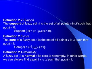
  • 1. Definition 2.2 Support The support of fuzzy set A is the set of all points x in X such that A(x) > 0: Support (A) = {x A(x) > 0}. Definition 2.3 core The core of a fuzzy set A is the set of all points x is X such that A(x) =1: Core(A) = {x A(x ) =1}. Definition 2.4 Normality A fuzzy set A is normal if its core is nonempty. In other words, we can always find a point x  X such that A(x) =1.
  • 2. Definition 2.5 Crossover points A crossover point of a fuzzy set A is a point x  X at which A(x)= 0.5: Crossover(A)={x A(x) = 0.5} Definition 2.6 Fuzzy singleton A fuzzy set whose support is a single point in X with A(x) = 1 is called a fuzzy singleton.
  • 3. Definition 2.7 -cut,strong -cut The -cut or -level set of a fuzzy set A is a crisp set defined by A’  = {x  A (x)  }. Using the notation for a level set, we can express the support and core of a fuzzy set A as Support(A) = A’ 0’ And Core(A)=A1’ Respectively.
  • 4. Definition 2.9 Fuzzy numbers A fuzzy number A is a fuzzy set in the real line (R) that satisfies the conditions for normality and convexity. Most (noncomposite) fuzzy sets used in the literature satisfy the conditions for normality and convexity, so fuzzy numbers are the most basic type of fuzzy sets.
  • 5. Definition 2.10 Bandwidths of normal and convex fuzzy sets For a normal and convex fuzzy set, the bandwidth of width is defined as the distance between the two unique crossover points: Width(A) = x2 – x1, Where A(x1) = A(2) = 0.5. Definition 2.11 Symmetry A fuzzy set A is symmetric if its MF is symmetric around a certain point x = c, namely,
  • 6. Definition 2.12 Open left, open right, closed A fuzzy set A is open left if limx A (x) =1 and limx+ A(x) = 0; open right if limx- A (x) = 0 and limx+A(x) = 1; and closed if limx-A (x) = limx+A (x) = 0.
  • 7. Law of contradiction A  =  Law of the excluded middle A  = X Idempotency A  A = A, A  A = A Involution = A Commutativity A  B = B  A, A  B = B  A Associativity (A  B)  C = A  (B  C ) (A  B)  C = A  ( B  C ) Distributivity A  (B  C ) = (A  B)  (A  C ) A  (B  C) = (A  B )  (A  C ) Absorption A  ( A  B ) = A A  ( A  B ) = A Absorption of Complements A  (  B) = A B A  (  B) = A B DeMorgan’s laws =  =  A A B A B A  B B A A A A A
  • 8. Cylindrical Extension Definition 2.24 Cylindrical extensions of one-dimensional fuzzy sets If A is a fuzzy set in X, then its cylindrical extension in X x Y is a fuzzy set c(A) defined by   XxY y x x A c A ). , /( ) ( ) ( 
  • 9. Projection Definition 2.25 Projection of fuzzy sets Let R be a two-dimensional fuzzy set on X x Y. Then the projections of R onto X and Y are defined as             X x y x R y X R / ) , ( max              Y y y x R x Y R / )] , ( max 
  • 10. Four of the most frequently used T-norm operators are Minimum Tmin(a, b) = min (a,b) = a  b. Algebraic product Tap (a, b) = ab. Bounded product Tbp(a, b) = 0  (a + b-1) a, if b= 1. Drastic product Tdp(a,b) = b, if a = 1. 0, if a,b  1.
  • 11. Corresponding to the four T-norm operators in the previous example, we have the following four T-conorm operators. Maximum : S(a, b) = max(a, b) = a  b. Algebraic sum : S(a, b) = a + b – ab. Bounded sum : S(a, b) = 1  (a + b ). a, if b = 0. Drastic sum: S(a,b) = b, if a = 0. 1, if a, b > 0.
  • 12. Yager [9]: For q > 0, Ty (a,b,q) = 1-min{1,[(1-a)q + (1-b)q]1/q}, Sy(a,b,q) = min{1,(aq +bq)1/q}. Dubois and Prade [4]: For   [0,1], TDP(a,b,) = ab/max {a,b,} SDP(a,b,) = [a+b – ab – min{a, b, (1-)} / max {1-a, 1 – b,} Hamacher [6]: For  > 0, TH (a, b, ) = ab / [+ (1-)(a + b – ab)], SH (a,b, ) = [a + b + ( -2) ab] / [1 + ( - 1) ab].
  • 13. Frank [5]: For s > 0, TF (a, b, s) = logs,[1 + (sa – 1)(sb –1)/(s –1)], SF (a, b, s) = 1 – logs[1 + (s1 – a –1) (s1-b-1)/(s-1)]. Sugeno [8]: For   -1, TS(a, b, ) = max{0, (+ 1)(a + b –1) - ab}, Ss (a, b, ) = min{1, a + b - ab}. Dombi [2]: For  > 0, TD (a, b, ) = SD(a, b, ) = , / 1 1 1 ] ) 1 ( ) 1 [( 1 1          b a , / 1 1 1 ] ) 1 ( ) 1 [( 1 1             b a
  • 14. 0 0.5 1 (a) Two fuzzy sets A and B A B 0 0.5 1 (b) T-norm of A and B 0 0.5 1 (c) T-conorm (S-norm) of A and B Figure. Schweizer and Sklar’s parameterized T-norms and T-conorms: (a) membership functions for fuzzy set A and B; (b) Tss(a,b,p) and (c) Sss (a, b, p) with p = ∞ (solid line), 1 (dashed line) and –1 (dash-dotted line).
  • 15. Definition 3.1 Extension principle Suppose that function f is a mapping from an n- dimensional Cartesian product space X1 x X2 x Xn to a one- dimensional universe Y such that y = f (x1,…,xn), and suppose Ai,…,An are n fuzzy sets in X1,…,Xn, respectively. Then the extension principle asserts that the fuzzy set B induced by the mapping f is defined by max [mini Ai(xi)], if f-1(y)0. B(y) = (x1,…,xn), (x1,…,xn) = f-1(y) 0, if f-1(y) =0.
  • 16. Example 3.1 Application of the extension principle to fuzzy sets with discrete universes Let A = 0.1/-2+0.4/-1+0.8/0 + 0.9/1 +0.3/2 And f (x) = x2 -3. Upon applying the extension principle, we have B = 0.1/1+0.4/-2+0.8/-3+ 0.9/ -2+ 0.3/1 = 0.8/ -3+ (0.4 V 0.9) / -2 + (0.1 V 0.3)/1 = 0.8/ -3 + 0.9/-2+ 0.3/1 where V represents max. Figure 3.1 illustrates this example.
  • 17. 0 0.111 0.200 0.273 0.333 R = 0 0 0.091 0.167 0.231 , 0 0 0 0.077 0.143 y -x R (x,y) = x+y+2 if y > x. 0, if y  x. Example 3.3 Binary fuzzy relations Let X = Y =R+ (the positive real line) and R = “y is much greater than x”, The MF of the fuzzy relation R can be subjectively defined as if X = {3,4,5} and Y = {3,4,5,6,7}, then it is convenient to express the fuzzy relation R as a relation matrix: where the element at row I and column j is equal to the membership grade between the ith element of X and jth element of y.
  • 18. Example 3.4 Max-min and max-product composition Let R1 = “x is relevant to y” R2 = “y is relevant to z” Be two fuzzy relations defined on X x Y and Y x Z, respectively, where X = {1, 2, 3} Y = {, , , }, and Z = {a, b}. Assume that R1 and R2 can be expressed as the following relation matrices:            2 . 0 3 . 0 8 . 0 6 . 0 9 . 0 8 . 0 2 . 0 4 . 0 7 . 0 5 . 0 3 . 0 1 . 0 1 R              2 . 0 7 . 0 6 . 0 5 . 0 3 . 0 2 . 0 1 . 0 9 . 0 2 R
  • 19. Now we want to find R1R2, which can be interpreted as a derived fuzzy relation “x is relevant to z” based on R1 and R2. For simplicity, suppose that we are only interested in the degree of relevance between 2 ( X) and a ( Z). If we adopt max-min composition, then On the other hand, if we choose max-product composition instead, we have ). min max ( 7 . 0 ) 7 . 0 , 5 . 0 , 2 . 0 , 4 . 0 max( ) 7 . 0 9 . 0 , 5 . 0 8 . 0 , 2 . 0 2 . 0 , 9 . 0 4 . 0 max( ) , 2 ( 2 1 n compositio by a R R           ). min max ( 63 .. 0 ) 63 . 0 , 40 . 0 , 04 . 0 , 36 . 0 max( ) 7 . 0 9 . 0 , 5 . 0 8 . 0 , 2 . 0 2 . 0 , 9 . 0 4 . 0 max( ) , 2 ( 2 1 n compositio by x x x x a R R      
  • 20. Extension principle on fuzzy sets with discrete universes 0.3 0.9 0.8 0.4 0.1 X Y f (x ) 1 0 -1 -2 -3 2 1 0 -1 -2
  • 21. Composition of fuzzy relations 1 2 3     a b X Y Z R1 R2 0.9 0.2 0.5 0.7 0.4 0.2 0.8 0.9
  • 22. From the preceding example, we can see that the term set consists of several primary terms (young, middle aged, old) modified by the negation (“not”) and/or the hedges (very, more or less, quite, extremely, and so forth), and then linked by connectives such as and, or, either, and neither. In the sequel, we shall treat the connectives, the hedges, and the negation as operators that change the meaning of their operands in a specified, context-independent fashion.
  • 23. Definition 3.6 Concentration and dilation of linguistic values Let A be a linguistic values characterized by a fuzzy set with membership function A(). Then AK is interpreted as a modified version of the original linguistic value expressed as In particular, the operation of concentration is defined as CON (A) = A2, While that of dilation is expressed by DIL(A) = A0.5. . / )] ( [ x x A k A x k   
  • 24. Following the definition in the previous chapter, we can interpret the negation operator NOT and the Connectives AND and OR as NOT(A) = ¬A = A AND B AB =  A OR B = AB =  Respectively, where A and B are two linguistic values whose meanings are defined by A() and B().   x A x x , / )] ( 1 [  x A x) ( [ , / )] ( x x B  x A x) ( [ , / )] ( x x B 
  • 25. Example 3.6 Constructing MFs for composite linguistic terms Let the meanings of the linguistic terms young and old be defined by the following membership functions: young (x) = bell(x,20,2,0)= old(x) = bell(x,30,3,100)= where x is the age of given person, with the interval [0,100] as the universe of discourse. Then we can construct MFs for the following composite linguistic terms: , 4 20 1 1          x , 6 30 100 1 1             x
  • 26.  more or less old = DIL (old) = old0.5  not young and not old = ¬young ¬old  young but not too young =young ¬young2  extremely old , 6 30 100 1 1 1 4 20 1 1 1 x x x x                                                                     . 6 30 100 1 1 x X x               . 2 20 1 1 1 4 20 1 1 x x x x                                                                                  
  • 27. Definition 3.8 Orthogonality A term set T = t1,…,tn of a linguistic variable x on the universe X is orthogonal if it fulfills the following property: where the ti’s are convex and normal fuzzy sets defined on X and these fuzzy sets make up the term set T.      n i X x x ti 1 , , 1 ) ( 
  • 28. If we interpret AB as A coupled with B, then R = AB = AxB = where is a T-norm operator and AB is used again to represent the fuzzy relation R. On the other hand, is AB is interpreted as A entails B, then it can be written as four different formulas:   XxY B A y x y x ), , /( ) ( ~ ) (    ~
  • 29. A entails B • Material implication: • Propositional calculus: •Extended propositional calculus: • Generalization of modus ponens: . B A B A R      ). ( B A A B A R       . ) ( B B A B A R        } 1 0 ) ( * ~ ) ( sup{ ) , (     c and y c x c y x B A R   
  • 30. Suppose that we adopt the first interpretation, “A coupled with B,” as the meaning of AB. Then four different fuzzy relations AB result from employing four of the most commonly used T-norm operators.  Rdp = A x B = XxY A(x) B(y)/(x,y), or F (a,b) = a b = .̂ a if b = 1. b if a = 1. 0 Otherwise. This formula uses the drastic product operator for conjunction .̂
  • 31. When we adopt the second interpretation, “A entails B,” as the meaning of AB, again there are number of fuzzy implication functions that are reasonable candidates. The following four have been proposed in the literature: • Ra =AB = XxY1 (1-A(x)+B(y)) /(x,y), or a(a,b) = 1(1- a+b). This is Zadeh’s arithmetic rule, which follows Equation (3.19) by using the bounded sum operator for . • Rmm =A(AB) = XxY (1-A(x))(A(x)B(y))/(x,y), or m(a,b) = (1-a)  (ab). This is Zadeh’s max-min rule, which follows Equation (3.20) by using max for .
  • 32.  Rs=AB=XxY ( 1-A(x))  B(y), or s(a,b) = (1-a)  b. This is Boolean fuzzy implication using max for . · R =XxY ( A(x B (y))/(x,y),where   . 1 . / ~ b a if b a if a b b a     This is Goguen’s fuzzy implication, which follows Equation (3.22) by using the algebraic product for the T-norm operator.  ~
  • 33. Specially, let A, c(A), B, and F be the MFs of A, c(A), B, and F, respectively, where c(A) is related to A through c(A) (x,y) = A(x). Then c(A)F(x,y) = min [c(A) (x,y), F(x,y)] = min [A (x), F(x,y)] by projecting c(A)  F onto the y-axis, we have B (y) = maxx min [A(x), F(x,y)] = Vx[A(x)  F(x,y)] This formula reduce to the max-min composition (see Definition 3.3 in Section 3.2) of two relation matrices if both A (a unary fuzzy relation) and F (a binary fuzzy relation) have finite universes of discourse. Conventionally, B is represented as B = A F,
  • 34. Definition 3.9 Approximate reasoning (fuzzy reasoning) Let A, A’, and B be fuzzy sets of X, X, and Y, respectively, Assume that the fuzzy implication AB is expressed as a fuzzy relation R on X x Y. Then the fuzzy set B induced by “x is A’” and the fuzzy rule “if x is A then y is B” is defined by μB’(y) = max min[μA’(x),μR(x,y)] = Vx[μA’(x)  μR(x,y)], or, equivalently, B’= A’ R = A’ (AB).
  • 35. The fuzzy rule in premise 2 can be put into the simpler form “A x B C.” Intuitively, this fuzzy rule can be transformed into a ternary fuzzy relation Rm Based on Mamdani’s fuzzy implication function, as follows: The resulting C’ is expressed as C’ = (A’ x B’)  (A x BC). Thus μC’(z) = Vx,y[μA’(x)  μB’(y)]  [μA(x)  μB(y)  μC(z)] = Vx,y{[μA’(x)  μB’(y)  μA(x)  μB(y)]}  μC(z) = {Vx[μA’(x)  μA(x)]}  {Vy[μB’(y)  μB(y)]}  μC(z) = (w1  w2)  μC(z), firing strength where w1 and w2 are the maxima of the MFs of A  A’ and B B’, respectively. ). , , /( ) ( ) ( ) ( ) ( ) , , ( z y x z c y B x A XxYxZ xC AxB C B A m R        
  • 36. Theorem 3.1 Decomposition method for calculating B’ C’ = (A’ x B’)  (A x B  C) = [A’ (AC)]  [B’  (BC)] Proof: μC’(z) = V x,y[μA’(x)  μB’(y)]  [μA(x)  μB(y)  μC(z)] = V x {μA’(x)  μB (y)  μC(z)  Vy[μB’(y)  μB(y)  μC(z)]} = μA’(x)  μB(y)  μC(z)  μB’ (BC)(y).
  • 37. To verify this inference procedure, let R1 = A1 x B1C1 and R2 = A2 x B2C2. Since the max-min composition operator  is distributive over the  operator, it follows that C’= (A’x B’)  (R1  R2) = [(A’x B’)  R1]  [ (A’x B’)R2] = C’1  C’2, where C’1 and C’2 are the inferred fuzzy sets for rules 1 and 2, respectively.
  • 38. In summary, the process of fuzzy reasoning or approximate reasoning can be divided into four steps: •Degrees of compatibility Compare the known facts with the antecedents of fuzzy rules to find the degrees of compatibility with respect to each antecedent MF. •Firing strength Combine degrees of compatibility with respect to antecendent MFs in a rule using fuzzy AND or OR operators to form a firing strength that indicates the degrees to which the antencedent part of the rule is satisfied. •Qualified (induced) consequent MFs Apply the firing strength to the consequent MF of a rule to generate a qualified consequent MF. (The qualified consequent MFs represent how the firing strength gets propagated and used in a fuzzy implication statement.) •Overall output MF Aggregate all the qualified consequent MFs to obtain an overall output MF.
  • 39. x is A1 y is B1 x is A2 y is Br x is Ar x is Br Rule 1 Rule 2 Rule 3 Aggregator Defuzzifier y (Fuzzy) (Fuzzy) (Fuzzy) (Fuzzy) w1 w2 w3 (Crisp) Figure Block diagram for a fuzzy inference system.
  • 40. •Centroid of area zCOA: zCOA = , ) ( ) (   z dz z A z zdz z A   •Bisector of area zBOA: zBOA satisfies    zBOA zBOA dz z A dz z A     , ) ( ) ( Mean of maximum zMOM: zMOM is the average of the maximizing z at which the MF reach a maximum μ*. In symbols, zMOM = where Z’ = {z A(z) = *}. In particular, if A(z) has a single maximum at z = z*, then zMOM =z*. Moreover, if μA(z) reaches its maximum whenever z  [zleft’zright] (this is the case in Figure 4.4), then zMOM = (zleft + zright)/2. The mean of maximum is the defuzzification strategy employed in Mamdani’s fuzzy logic controllers [6]. , ' '   z dz z zdz
  • 41. • Smallest of maximum zSOM:zSOM is the minimum (in terms of magnitude) of the maximizing z. • Largest of maximum zLOM:zLOM is the maximum (in term magnitude) of the maximizing z. Because of their obvious bias, zSOM and LOM are not used as often as the other three defuzzification methods.
  • 42. Example 4.1 Single-input single-output Mamdani fuzzy model An example of a single-input single-output Mamdani fuzzy model with three rules can be expressed as If X is small then Y is small. If X is medium then Y is medium. If X is large then Y is large.
  • 43. -10 -8 -6 -4 -2 0 2 4 6 8 10 0 0.2 0.4 0.6 0.8 1 X Membership Grades small medium large 0 1 2 3 4 5 6 7 8 9 10 0 0.2 0.4 0.6 0.8 1 Y Membership Grades small medium large -10 -8 -6 -4 -2 0 2 4 6 8 10 0 1 2 3 4 5 6 7 8 9 10 X Y Figure Single-input single-output Mamdani fuzzy model in Example 4.1: (a) antecendent and consequent MFs; (b) overall input-output curve. (MATLAB file: mam1.m)
  • 44. Example .4.2 Two-input single-output Mamdani fuzzy model An example of a two-input single-output Mamdani fuzzy model with four rules can be expressed as If X is small and Y is small then Z is negative large. If X is small and Y is large then Z is negative small. If X is large and Y is small then Z is positive small. If X is large and Y is large then Z is positive large.
  • 45. -5 -4 -3 -2 -1 0 1 2 3 4 5 0 0.5 1 X Membership Grades small large -5 -4 -3 -2 -1 0 1 2 3 4 5 0 0.5 1 Y Membership Grades small large -5 -4 -3 -2 -1 0 1 2 3 4 5 0 0.5 1 Z Membership Grades large negative small negative small positive large positive -5 0 5 -5 0 5 -3 -2 -1 0 1 2 3 X Y Z Figure Two-input single-output Mamdani fuzzy model in Example 4.2(a) antecendent and consequent MFs; (b) overall input-output surface. (MATLAB file: mam2.m)
  • 46. Therefore, to completely specify the operation of a Mamdani fuzzy inference system, we need to assign a function for each of the following operators: • AND operator (usually T-norm) for calculating the firing strength of a rule with AND’ed antecendents. • OR operator (usually T-conorm) for calculating the firing strength of a rule with OR’ed antecendents. • Implication operator (usually T-norm) for calculating qualified consequent MFs based on given firing strength. • Aggregate operator (usually T-conorm) for aggregating qualified consequent MFs to generate an overall output MF. • Defuzzification operator for transforming an output MF to crisp single output value.
  • 47. Theorem 4.1 Computation shortcut for Mamdani fuzzy inference systems Under sum-product composition, the output of a Mamdani fuzzy inference system with centroid defuzzification is equal to the weighted average of the centroids of consequent MFs, where each of the weighting factors is equal to the product of a firing strength and the consequent MF’s area. Proof: We shall prove this theorem for a fuzzy inference system with two rules. By using product and sum for implication and aggregate operators, respectively, we have μC’(z) = w1μC1(z) + w2μC2(z).
  • 48. A1 A2 x x x   B1 y  B2 x  Min or Product Weighted Average W1 W2 z1 = p1 x + q1 y + r1 z2 = p2 x + q2 y + r2 2 1 2 2 1 1 w w z w z w z    Figure The Sugeno fuzzy model.
  • 49. (Note that the precending MF could have values greater than 1 at certain points.) The crisp output under centroid defuzzification is where ai (=zCi(z)dz) and zi are the area and centroid of the consequent MF Ci(z), respectively.    z dc z C z zdz z C COA z ) ( ' ) ( '          dz z C w dz z C w zdz z C w zdz z C W ) ( 2 2 ) ( 1 1 ) ( 2 2 ) ( 1 1     2 2 1 1 2 2 2 1 1 1 a w a w z a w z a W    ) ) ( ) ( (    z dz z i C z zdz z i C  
  • 50. Example 4.3 Fuzzy and nonfuzzy rule set-a comparison An example of a single-input Sugeno fuzzy model can be expressed as If Xis small then y = 0.1X + 6.4. If X is medium then Y = -0.5X+4. If X is large then Y = X-2.
  • 51. -10 -5 0 5 10 0 0.2 0.4 0.6 0.8 1 X Membership Grades small medium large (a) Antecedent MFs for Crisp Rules -10 -5 0 5 10 0 2 4 6 8 X Y (b) Overall I/O Curve for Crisp Rules -10 -5 0 5 10 0 0.2 0.4 0.6 0.8 1 X Membership Grades small medium large (c) Antecedent MFs for Fuzzy Rules -10 -5 0 5 10 0 2 4 6 8 X Y (d) Overall I/O Curve for Fuzzy Rules Figure Comparison between fuzzy and non fuzzy rules in Example 4.3: (a) Antecendent MFs and (b) input-output curve for nonfuzzy rules; (c) Antencendent MFs and (d) input-output curve for fuzzy rules. (MATLAB file:sug1.m)
  • 52. Example 4.4 Two-input single-output Sugeno fuzzy model An example of a two-input single-output Sugeno fuzzy model with four rules can be expressed as If X is small and Y is small then z = -x+y+1. If X is small and Y is large then z = -y+3. If X is large and Y is small then z =-x+3. If X is large and Y is large then z = x+y +2.
  • 53. -5 -4 -3 -2 -1 0 1 2 3 4 5 0 0.2 0.4 0.6 0.8 1 X Membership Grades Small Large -5 -4 -3 -2 -1 0 1 2 3 4 5 0 0.2 0.4 0.6 0.8 1 Y Membership Grades Small Large Figure Two-input single-output Sugeno fuzzy model in Example 4.4: (a) antecendent and consequent MFs; (b) overall input-output surface. (MATLAB file sug2.m)
  • 55. An example of a single-input Tsukamoto fuzzy model can be expressed as If X is small then Y is C1 If X is medium then Y is C2 If X is large then Y is C3 Where the antecendent MFs for “small,” “medium,” and “large” are shown in Figure 4.12(a), and the consequent MFs for “C1,” “C2,” and “C3” are shown in Figure 4.12(b). The overall input-output curve, as shown in Figure 4.12(d), is equal to ( ) / ( ), where fi is the output of each rule induced by the firing strength wi and MF for Ci. If we plot each rule’s output fi as a function of x, we obtain Figure 4.12(c), which is not quite obvious from the original rule base and MF plots.   3 1 1 1 i f w  3 1 1 i w
  • 56. -10 -5 0 5 10 0 0.2 0.4 0.6 0.8 1 X Membership Grades small medium large (a) Antecedent MFs 0 5 10 0 0.2 0.4 0.6 0.8 1 Y Membership Grades C1 C2 C3 (b) Consequent MFs Figure Single-input single output Tsukamoto fuzzy model in Example 4.4:(a) antecendent MFs; (b) consequent MFs; (c) each rule’s output curves; (d) overall input-output curve. ( MATLAB file: tsu1.m)
  • 57. (a) (b) (c) Figure Various methods for partitioning the input space: (a) grid partition; (b) tree partition; (c) scatter partition.
  • 58. Generally speaking, the standard method of constructing a fuzzy inference system, a process usually called fuzzy modeling, has the following features: • The rule structure of a fuzzy inference system makes it easy to incorporate human expertise about the target system directly into the modeling process. Namely, fuzzy modeling takes advantage of domain knowledge that might not be easily or directly employed in other modeling approaches. • When the input-output data of a target system is available, conventional system identification techniques can be used for fuzzy modeling. In other words, the use of numerical data also plays an important role in fuzzy modeling, just as in other mathematical modeling methods.
  • 59. Conceptually, fuzzy modeling can be pursued in two stages, which are not totally disjoint. The first stage is the identification of the surface structure, which included the following tasks: 1. Select relevants input and output variables. 2. Choose a specific type of fuzzy inference system. 3. Determine the number of linguistic terms associated with each input and output variables. (For a Sugeno model, determine the order of consequent equations.) 4. Design a collection of fuzzy if-then rules.
  • 60. Specially, the identification of deep structure includes the following task : 1. Choose an appropriate family of parameterized MFs(see Section 2.4). 2. Interview human experts familiar with the target systems to determine the parameters of the MFs used in the rule base. 3. Refine the parameters of the MFs using regression and optimization techniques.
  • 61. Beberapa tipe teknik kendali adaptif berbeda hanya dalam cara parameter pengendali disesuaikan. Pada dasarnya ada 4 pendekatan berbeda untuk kendali adapatif konvensional, yaitu: 1.Pendekatan Gain Scheduling 2.Kendali Adaptif Referensi Model 3.Pendekatan Self-tuning 4.Pendekatan Kendali Stochastic
  • 63. Reference Model Controller Plant Reference input (r) Adaptive laws Control input (u) Plant output Yp Model output Ym Gambar Teknik Kendali Adaptif Referensi Model
  • 64. Controller Plant Reference input (r) Estimator Controller input (u) output (Y) Design criteria Controller Parameter Estimated Parameters Gambar Teknik Self-Tuning
  • 68. Trained NN (A) error Plant + - NN (B) Controller U(k) Yd(k+1) (B = copy of A) Y(k+1) Gambar Arsitektur Pembelajaran tidak Langsung
  • 69. Plant + - Controller U output, Y Input, r e model NN Predicted control signal Gambar Struktur Kendali Imitasi
  • 71. C C T T U(0) Back - Propagation C T X (0) X (1) U(1) X(NT-1) U(NT-1) X(NT) Xd(NT) eNT + - Gambar Training Pengendali NN
  • 72. Control NN Model NN Plant Critic NN Input output . Gambar Struktur Kendali BAC
  • 76. 1 0 0 0 1 0 1 1 1 0 1 1 1 0 1 0 1 1 1 1 0 0 1 0 + + Crossover site Gambar Crossover algoritma genetik standar: Dua mating individual (kiri) dan keturunan (kanan)
  • 78. Model NN Delay Plant Predicted Output Output Input 5  t to t U t U ) 6 (  t m Y ) 6 (  t p Y   Gambar Struktur Tapped-Delay-Line
  • 79. Delay Delay ) 3 ( 1  t Y ) 3 ( 2  t Y ) 2 ( 1  t Y ) 2 ( 2  t Y ) ( 1 t U ) ( 2 t U ) 1 ( 1  t U ) 1 ( 2  t U ) 2 ( 1  t U ) 2 ( 2  t U Gambar Arsitektur Umpan balik Output
  • 80. ) 3 ( 1  t Y ) 3 ( 2  t Y ) 1 ( 1  t U ) 1 ( 2  t U ) 1 ( 3  t U Output Layer Hidden Layer Context Layer Input Layer Gambar Arsitektur Jaringan Recurrent Dasar
  • 82. Linear Feedback Sliding Netw ork Modulate Plant ) (t xd ) (t xn d ) (t x ) (t U pd ) (t U gl ) (t Uad ) (t x    Gambar Pengendali Adaptif Langsung dikemukakan oleh Slotine dan Sanner
  • 83. G G G G ) ( 1 t x ) ( 2 t x 1 W 2 Ŵ 1 ˆ A h 1 ˆ A b ) ( 1 t a  ad t u ) (     Gambar Struktur komponen adaptif dari aturan kendali untuk plant gain nonunity
  • 84. Controller NNC Nonlinear Plant TDL TDL TDL TDL Identif ication Model Ref erence Model Z U i e m Y i e p Y r c e     Gambar Kendali Adaptif tidak Langsung dengan Menggunakan Jaringan Neural
  • 85. Ng Nc g z-1 f z-1 Nf -Nf 0.6 Reference Model        ) (k r            ) (k ec ) (k e identification Model ) ( ˆ k Y Gambar Pendekatan Narendra
  • 86. Inverse Dynamics Model Plant Forward Dynamics Model error in Control Command error in Trajectory + - ) (t d  ) (t  ) (t Ti Gambar Pemodelan Forward dan Inverse
  • 87. ) ( 1 1 k X ) ( 1 2 k X 1 11 S 1 11 V 3 12  3 1 S Memory Neuron Network Neuron S dan V ----- Weight Gambar Struktur Jaringan Neural Memori
  • 89. Research Topics  Type 2 Fuzzy Logic Systems – Jerry M. Mendel dkk.