Gridding av klimadata
•Descargar como PPTX, PDF•
0 recomendaciones•117 vistas

Metoden bak gridding av klimadata som benyttes av Meteorologisk institutt forklart av Ole Einar Tveito

Recomendados
Recomendados
Más contenido relacionado
La actualidad más candente
La actualidad más candente (19)
Similar a Gridding av klimadata
Similar a Gridding av klimadata (20)
Más de Hans Olav Hygen
Más de Hans Olav Hygen (20)
Último
Último (20)
Gridding av klimadata
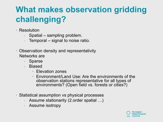
- 1. What makes observation gridding challenging? · Resolution - Spatial – sampling problem. - Temporal – signal to noise ratio. · Observation density and representativity Networks are - Sparse - Biased · Elevation zones · Environment/Land Use: Are the environments of the observation stations representative for all types of environments? (Open field vs. forests or cities?) · Statistical assumption vs physical processes - Assume stationarity (2.order spatial …) - Assume isotropy
- 2. Standard deviation of terrain ~10 km influence area Elevation
- 3. The distribution of elevation 0 500 1000 1500 2000 0.00.20.40.60.81.0 Elevation Frequency
- 4. The distribution of elevation 0 500 1000 1500 2000 0.00.20.40.60.81.0 Elevation Frequency
- 5. The distribution of elevation & temperature stations 0 500 1000 1500 2000 0.00.20.40.60.81.0 Elevation Frequency
- 6. The distribution of elevation & temperature stations 0 500 1000 1500 2000 0.00.20.40.60.81.0 Elevation Frequency 57/195 masl 480/554 masl
- 7. Gridding challenges (i) Observation gridding is basically based on statistical relations • Quality depends on station density and representativity of the station network. The choice of external predictor should be based on a good understanding of the physical processes of the predictand (on a local scale).
- 8. Make the observations stationary Two approaches: • Anomaly approach: • Analysis of normalized (relative) values (% of normal, deviation from normal): The normals include the non-stationarity, and by normalizing by the normals, the values are in principle stationary. Any statistical interpolation method can be applied more or less automatically. • Detrending approach: • Analysis of absolute values Find, and remove trends caused by topography and/or other terrain or surface characteristics. The residual field can be interpolated by using e.g. kriging or other suitable interpolation techniques. This approach is often referred to as residual kriging or detrended kriging.
- 9. Interpolation of monthly anomalies · Precipitation sums: RRanom = RR / RRmean · Temperature: TManom = TM – TMmean · Grids of normal values are necessary to obtain absolute values. · Interpolation method: E.g. Topogrid - Discretised thin plate spline technique (Hutchinson, 1988,1989, Wahba, 1990) - Local interpolator - Comparison with kriging and IDW shows similar performance. The input ensure robust estimates! - Gives smooth surfaces, (avoiding strange spatial patterns)!
- 11. Time series of climate grids Use the zonal statistics function in a GIS to establish areal statistics. -2 -1.5 -1 -0.5 0 0.5 1 1.5 2 2.5 1900 1910 1920 1930 1940 1950 1960 1970 1980 1990 2000 2010 Norge - Årstemperatur Norge 10 per. Mov. Avg. (Norge) Linear (Norge)