Changing variable

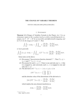
1. THE CHANGE OF VARIABLE THEOREM
STEVEN J MILLER (SJM1@WILLIAMS.EDU)
1. STATEMENT
Theorem 1.1 (Change of Variables Formula in the Plane). Let 𝑆 be an
elementary region in the 𝑥𝑦-plane (such as a disk or parallelogram for ex-
ample). Let 𝑇 : ℝ2
→ ℝ2
be an invertible and differentiable mapping, and
let 𝑇(𝑆) be the image of 𝑆 under 𝑇. Then
∫ ∫
𝑆
1 ⋅ 𝑑𝑥𝑑𝑦 =
∫ ∫
𝑇(𝑆)
1 ⋅
∂𝑥
∂𝑢
∂𝑦
∂𝑣
−
∂𝑥
∂𝑣
∂𝑦
∂𝑢
𝑑𝑢𝑑𝑣,
or more generally
∫ ∫
𝑆
𝑓(𝑥, 𝑦) ⋅ 𝑑𝑥𝑑𝑦 =
∫ ∫
𝑇(𝑆)
𝑓
(
𝑇−1
(𝑢, 𝑣)
)
⋅
∂𝑥
∂𝑢
∂𝑦
∂𝑣
−
∂𝑥
∂𝑣
∂𝑦
∂𝑢
𝑑𝑢𝑑𝑣.
Some notes on the above:
(1) We assume 𝑇 has an inverse function, denoted 𝑇−1
. Thus 𝑇(𝑥, 𝑦) =
(𝑢, 𝑣) and 𝑇−1
(𝑢, 𝑣) = (𝑥, 𝑦).
(2) We assume for each (𝑥, 𝑦) ∈ 𝑆 there is one and only one (𝑢, 𝑣) that
it is mapped to, and conversely each (𝑢, 𝑣) is mapped to one and
only one (𝑥, 𝑦).
(3) The derivative of 𝑇−1
(𝑢, 𝑣) = (𝑥(𝑢, 𝑣), 𝑦(𝑢, 𝑣)) is
(𝐷𝑇−1
)(𝑢, 𝑣) =
( ∂𝑥
∂𝑢
∂𝑥
∂𝑣
∂𝑦
∂𝑢
∂𝑦
∂𝑣
)
,
and the absolute value of the determinant of the derivative is
det
(
𝐷𝑇−1
)(𝑢, 𝑣)
)
=
∂𝑥
∂𝑢
∂𝑦
∂𝑣
−
∂𝑥
∂𝑣
∂𝑦
∂𝑢
,
which implies the area element transforms as
𝑑𝑥𝑑𝑦 =
∂𝑥
∂𝑢
∂𝑦
∂𝑣
−
∂𝑥
∂𝑣
∂𝑦
∂𝑢
𝑑𝑢𝑑𝑣.
Date: April 14, 2011.
1

2. 2 STEVEN J MILLER (SJM1@WILLIAMS.EDU)
(4) Note that 𝑓 takes as input 𝑥 and 𝑦, but when we change variables
our new inputs are 𝑢 and 𝑣. The map 𝑇−1
takes 𝑢 and 𝑣 and gives 𝑥
and 𝑦, and thus we need to evaluate 𝑓 at 𝑇−1
(𝑢, 𝑣). Remember that
we are now integrating over 𝑢 and 𝑣, and thus the integrand must be
a function of 𝑢 and 𝑣.
(5) Note that the formula requires an absolute value of the determinant.
The reason is that the determinant can be negative, and we want to
see how a small area element transforms. Area is supposed to be
positively counted. Note in one-variable calculus that
∫ 𝑏
𝑎
𝑓(𝑥)𝑑𝑥 =
−
∫ 𝑎
𝑏
𝑓(𝑥)𝑑𝑥; we need the absolute value to take care of issues such
as this.
(6) While we stated 𝑇 is a differentiable mapping, our assumptions im-
ply 𝑇−1
is differentiable as well.
2. SKETCH OF PROOF
The Change of Variable Theorem (or Formula) is one of the most impor-
tant results of multivariable calculus. The reason is that numerous problems
have a natural coordinate system where, if we look at it from the right per-
spective, the analysis greatly simplifies. It is thus very important to be able
to convert from one coordinate system to another and be able to exploit the
advantages of each.
Our first example was mapping the unit square to a rectangle (see Figure
1). Note the original square, 𝑆, has area 1 and the region it maps to, 𝑇(𝑆),
has area 6. Thus 𝑑𝑥𝑑𝑦 corresponds to 1
6
𝑑𝑢𝑑𝑣. If we compute the derivative
matrix associated to 𝑇−1
, since
𝑥(𝑢, 𝑣) = 𝑢/2 and 𝑦(𝑢, 𝑣) = 𝑣/3,
we find ( ∂𝑥
∂𝑢
∂𝑥
∂𝑣
∂𝑦
∂𝑢
∂𝑦
∂𝑣
)
=
( 1
2
0
0 1
3
)
,
which has a determinant of 1/6. This verifies the formula’s prediction,
namely that the exchange rate from 𝑥𝑦-space to 𝑢𝑣-space is 1/6. In other
words, ∫ ∫
𝑆
1 ⋅ 𝑑𝑥𝑑𝑦 =
∫ ∫
𝑇(𝑆)
1
6
⋅ 𝑑𝑢𝑑𝑣;
clearly we don’t expect
∫ ∫
𝑆
1 ⋅ 𝑑𝑥𝑑𝑦 to equal
∫ ∫
𝑇(𝑆)
⋅𝑑𝑢𝑑𝑣; the absolute
value of the determinant of the derivative matrix gives the exchange rate.
We now sketch the proof. It will involve several of the major concepts
we’ve discussed throughout the semester, from the cross product to deter-
minants and areas to the definition of the derivative being that the tangent

3. THE CHANGE OF VARIABLE THEOREM 3
FIGURE 1. Mapping the unit square via u = 2x and v = 3y
FIGURE 2. Mapping of the general case: 𝑥(𝑢, 𝑣) and
𝑦(𝑢, 𝑣). Note: to save time I’ve written 𝑢0 +𝑑𝑢 for 𝑢0 +Δ𝑢,
and similarly for the 𝑣’s, above.
plane is a great approximation. Recall we have
𝑇−1
(𝑢, 𝑣) = (𝑥(𝑢, 𝑣), 𝑦(𝑢, 𝑣)).
We want to see what a small rectangle in 𝑢𝑣-space corresponds to in 𝑥𝑦-
space; see Figure 2. We want to see where the four corners of the rectangle
in the 𝑢𝑣-plane are mapped. Recall that if we have a function 𝑓(𝑢, 𝑣), then
𝑓(𝑢, 𝑣) = 𝑓(𝑢0, 𝑣0) + (∇𝑓)(𝑢0, 𝑣0) ⋅ (𝑢 − 𝑢0, 𝑣 − 𝑣0) + small

4. 4 STEVEN J MILLER (SJM1@WILLIAMS.EDU)
if (𝑢, 𝑣) is close to (𝑢0, 𝑣0). There are many ways to look at this. It is a
Taylor expansion, it is a definition of the derivative, it is taking a directional
derivative.
As 𝑇−1
is differentiable, we can write
𝑥(𝑢, 𝑣) = 𝑥(𝑢0, 𝑣0) + (∇𝑥)(𝑢0, 𝑣0) ⋅ (𝑢 − 𝑢0, 𝑣 − 𝑣0) + small
𝑦(𝑢, 𝑣) = 𝑦(𝑢0, 𝑣0) + (∇𝑦)(𝑢0, 𝑣0) ⋅ (𝑢 − 𝑢0, 𝑣 − 𝑣0) + small, ,
so long as (𝑢, 𝑣) is close to (𝑢0, 𝑣0). This is simply the definition of the de-
rivative in several variables, namely the statement that we can approximate
a complicated function locally by a plane. What makes it a little confusing
is that 𝑥 is now our function name, not a coordinate (this is why we con-
sidered the example with a function 𝑓 above). Thus, while the square with
lengths Δ𝑢 and Δ𝑣 in 𝑢𝑣-space doesn’t map to exactly a square, rectangle
or parallelogram in 𝑥𝑦-space, it maps to almost a parallelogram. Let’s see
where the four corners of the rectangle map to; expanding the gradient we
find
𝑥(𝑢, 𝑣) = 𝑥0 +
∂𝑥
∂𝑢
(𝑢 − 𝑢0) +
∂𝑥
∂𝑣
(𝑣 − 𝑣0) + small
𝑦(𝑢, 𝑣) = 𝑦0 +
∂𝑦
∂𝑢
(𝑢 − 𝑢0) +
∂𝑦
∂𝑣
(𝑣 − 𝑣0) + small.
Note that 𝑥(𝑢0, 𝑣0) is what we’re calling 𝑥0 and 𝑦(𝑢0, 𝑣0) is what we’re
calling 𝑦0, the base point of the square. For definiteness we are assuming
the four corner’s orientation is preserved under the mapping (we had to
choose how to draw / discuss things). We have
(𝑥(𝑢0 + Δ𝑢, 𝑣0), 𝑦(𝑢0 + Δ𝑢, 𝑣0)) =
(
𝑥0 +
∂𝑥
∂𝑢
Δ𝑢, 𝑦0 +
∂𝑦
∂𝑢
Δ𝑢
)
(𝑥(𝑢0, 𝑣0 + Δ𝑣), 𝑦(𝑢0, 𝑣0 + Δ𝑣)) =
(
𝑥0 +
∂𝑥
∂𝑣
Δ𝑣, 𝑦0 +
∂𝑦
∂𝑣
Δ𝑣
)
.
The original rectangle in 𝑢𝑣-space had sides given by the vectors (𝑢0 +
Δ𝑢, 𝑣0) − (𝑢0, 𝑣0) and (𝑢0, 𝑣0 + Δ𝑣) − (𝑢0, 𝑣0). Thus the area is equivalent
to that of a rectangle given by the vectors (Δ𝑢, 0) and (0, Δ𝑣), for an area
of Δ𝑢Δ𝑣.
What about the region it is mapped to? It is essentially a parallelogram;
this is the content of the function 𝑇−1
being differentiable. The side (𝑢0 +
Δ𝑢, 𝑣0) − (𝑢0, 𝑣0) which was equivalent to the vector (Δ𝑢, 0) corresponds
to
(𝑥(𝑢0 + Δ𝑢, 𝑣0) − (𝑥0, 𝑦0)),
which is just (
∂𝑥
∂𝑢
Δ𝑢,
∂𝑦
∂𝑢
Δ𝑢
)
;

5. THE CHANGE OF VARIABLE THEOREM 5
similarly the other side corresponds to
(
∂𝑥
∂𝑣
Δ𝑣,
∂𝑦
∂𝑣
Δ𝑣
)
.
To find the area of a parallelogram with sides −→𝑤 1 and −→𝑤 2 we need only
take the cross product. We must be careful, though. The cross product takes
as input two vectors with three components and outputs a vector with three
components. We can consider our vectors as living in three-dimensional
space by appending a zero as the third component, and then the area of the
parallelogram is the length of the cross product. We must compute
(
∂𝑥
∂𝑢
Δ𝑢,
∂𝑦
∂𝑢
Δ𝑢, 0
)
×
(
∂𝑥
∂𝑣
Δ𝑣,
∂𝑦
∂𝑣
Δ𝑣, 0
)
.
Recall this is given by
−→
𝑖
−→
𝑗
−→
𝑘
∂𝑥
∂𝑢
Δ𝑢 ∂𝑦
∂𝑢
Δ𝑢 0
∂𝑥
∂𝑣
Δ𝑣 ∂𝑦
∂𝑣
Δ𝑣 0
=
(
0, 0,
(
∂𝑥
∂𝑢
∂𝑦
∂𝑣
−
∂𝑥
∂𝑣
∂𝑦
∂𝑢
)
Δ𝑢Δ𝑣
)
,
and the length is clearly just
∂𝑥
∂𝑢
∂𝑦
∂𝑣
−
∂𝑥
∂𝑣
∂𝑦
∂𝑢
Δ𝑢Δ𝑣,
or equivalently
𝑑𝑥𝑑𝑦 ∼
∂𝑥
∂𝑢
∂𝑦
∂𝑣
−
∂𝑥
∂𝑣
∂𝑦
∂𝑢
Δ𝑢Δ𝑣.
The outline above highlights the key ideas in the proof. One needs to
perform a careful analysis of the error terms, but the main points are above.
The idea is that locally any differentiable map is linear (and takes rectan-
gles to parallelograms), and then we piece the contributions over the entire
region together. The absolute value of the determinant of the derivative map
gives us the exchange rate between the two different areas.
3. SPECIAL CASES
Theorem 3.1 (Change of Variables Theorem: Polar Coordinates). Let
𝑥 = 𝑟 cos 𝜃, 𝑦 = 𝑟 sin 𝜃
with 𝑟 ≥ 0 and 𝜃 ∈ [0, 2𝜋); note the inverse functions are
𝑟 =
√
𝑥2 + 𝑦2, 𝜃 = arctan(𝑦/𝑥).

6. 6 STEVEN J MILLER (SJM1@WILLIAMS.EDU)
Let 𝐷 be an elementary region in the 𝑥𝑦-plane, and let 𝐷∗
be the corre-
sponding region in the 𝑟𝜃-plane. Then
∫ ∫
𝐷
𝑓(𝑥, 𝑦)𝑑𝑥𝑑𝑦 =
∫ ∫
𝐷∗
𝑓(𝑟 cos 𝜃, 𝑟 sin 𝜃)𝑟𝑑𝑟𝑑𝜃.
For example, if 𝐷 is the region 𝑥2
+ 𝑦2
≤ 1 in the 𝑥𝑦-plane then 𝐷∗
is
the rectangle [0, 1] × [0, 2𝜋] in the 𝑟𝜃-plane.
Theorem 3.2 (Change of Variables Theorem: Cylindrical Coordinates). Let
𝑥 = 𝑟 cos 𝜃, 𝑦 = 𝑟 sin 𝜃, 𝑧 = 𝑧
with 𝑟 ≥ 0, 𝜃 ∈ [0, 2𝜋) and 𝑧 arbitrary; note the inverse functions are
𝑟 =
√
𝑥2 + 𝑦2, 𝜃 = arctan(𝑦/𝑥), 𝑧 = 𝑧.
Let 𝐷 be an elementary region in the 𝑥𝑦𝑧-plane, and let 𝐷∗
be the corre-
sponding region in the 𝑟𝜃𝑧-plane. Then
∫ ∫ ∫
𝐷
𝑓(𝑥, 𝑦, 𝑧)𝑑𝑥𝑑𝑦𝑑𝑧 =
∫ ∫ ∫
𝐷∗
𝑓(𝑟 cos 𝜃, 𝑟 sin 𝜃, 𝑧)𝑟𝑑𝑟𝑑𝜃𝑑𝑧.
Theorem 3.3 (Change of Variables Theorem: Spherical Coordinates). Let
𝑥 = 𝜌 sin 𝜙 cos 𝜃, 𝑦 = 𝜌 sin 𝜙 sin 𝜃, 𝑧 = 𝜌 cos 𝜙
with 𝜌 ≥ 0, 𝜃 ∈ [0, 2𝜋] and 𝜙 ∈ [0, 𝜋). Note that the angle 𝜙 is the angle
made with the 𝑧-axis; many books (such as physics texts) interchange the
role of 𝜙 and 𝜃. Let 𝐷 be an elementary region in the 𝑥𝑦𝑧-plane, and let 𝐷∗
be the corresponding region in the 𝜌𝜃𝜙-plane. Then
∫ ∫ ∫
𝐷
𝑓(𝑥, 𝑦, 𝑧)𝑑𝑥𝑑𝑦𝑑𝑧 =
∫ ∫ ∫
𝐷∗
𝑓(𝜌 sin 𝜙 cos 𝜃, 𝜌 sin 𝜙 sin 𝜃, 𝜌 cos 𝜙)𝜌2
sin(𝜙)𝑑𝜌𝑑𝜃𝑑𝜙.
Note that the most common mistake is to have incorrect bounds of inte-
gration.