1. 2PA3 EXPERIMENT 3b version 23Sep03
THE JOULE-THOMSON EXPERIMENT
OBJECTIVE: Measure the Joule-Thomson coefficient of carbon dioxide. Compare
the calculated value with that calculated from the equation of state.
1. INTRODUCTION:
One of the fundamental assumptions of the Kinetic Theory of Gases is that
there is no attraction between molecules of the gas. An ideal gas may be regarded as
one for which the molecular attraction is negligible. The fact that gases may be
liquefied implies that the molecules of a gas attract one another. This attraction was
studied by J. L. Gay-Lussac (1807) and J. P. Joule (1843) who investigated the
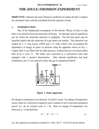
dependence of energy of gases on pressure using the apparatus shown in Fig. 1.
Copper bulb A was filled with air under pressure, isolated from an evacuated similar
bulb B by a valve, V. The bulbs were immersed in a well-stirred water bath
equipped with a sensitive thermometer. After thermal equilibrium had been
established, valve V was opened to allow the gas to expand into bulb B.
Figure 1 Joule Apparatus
No change in temperature was detected. In Joule's words, "no change of temperature
occurs when air is allowed to expand in such a manner as not to develop mechanical
power" (i.e. do no external work, w = 0). Since no change of temperature was
observed, q = 0 and therefore
dU = dq = dw = 0 (1)
(i.e. the expansion occurred at constant U). Now, for U = U(V,T) it can be shown

2. Expt. 3b Joule-Thomson Experiment 2
that
    
U
V T
=−
U
T V
T
V U
(2)
Joule's observation that
 
T
V U
=0
implies (from eqn. (2) )
 
U
V T
=0
or the energy of a gas is a function of temperature alone, independent of volume (and
therefore of pressure) at constant temperature. Because the system used by Joule had
a very large heat capacity compared with the heat capacity of air, the small change of
temperature that took place was not observed. Actually the gas in A warmed up
slightly and the one which had expanded into B was somewhat cooler and when
thermal equilibrium was finally established the gas was at a slightly different
temperature from that before the expansion. Thus
 
U
V T
≠0
It is only when the pressure of the gas before expansion is reduced that the
temperature change becomes smaller and smaller. Thus we can deduce that in the
limit of zero pressure the effect would be zero and the energy of the gas would be
independent of volume. An ideal gas can be defined by
PV = nRT
lim
P0   U
V T
=0 (3)
In fact any of the following are valid for an ideal gas
       
U
V T
=
U
P T
=
H
V T
=
H
P T
=0 (4)
THE JOULE-THOMSON EXPERIMENT.
The study of the dependence of the energy and enthalpy of real gases on volume
(pressure) was done by Joule in association with Thomson who devised a different
procedure. They allowed gas to expand freely through a porous plug, or frit.

3. Expt. 3b Joule-Thomson Experiment 3
Figure 2 Principle of the Joule-Thomson apparatus
As shown in Fig. 2, the gas expands from a pressure P1 to pressure P2 by the
throttling action of the porous plug. The entire system is thermally insulated so the
expansion occurs adiabatically, i.e.
1 q = 0
Gas is allowed to flow continuously through the porous plug, and when steady state
conditions have been reached the temperatures of the gas before and after expansion,
T1 and T2, are measured directly with sensitive thermocouples. The following
argument shows that this expansion occurs at constant enthalpy. Consider the
expansion of a fixed mass of gas, through the frit. This may be treated by
considering a system defined by the imaginary pistons shown in Fig. 2. The gas
occupies a volume V1 at a pressure P1 and temperature T1 before the expansion and a
volume V2 at P2, T2 after the expansion. What is the work done in this process?
Compression of the imaginary piston on the LHS leads to work done (by the
surroundings on the system) of
0
− p1  V where  V =∫V dV =−V 1 or w LHS =P 1 V 1
1
Similarly, expansion of the imaginary piston on the RHS leads to work done on the
system by the surroundings of
2 - P 2 V where V = V 2 - 0 = V 2 or w LHS = - P2 V 2
The total work done on the gas system during the expansion is then
3 w = wLHS + wRHS = + P1 V 1 - P2 V 2

4. Expt. 3b Joule-Thomson Experiment 4
The overall change in internal energy of the gas during the adiabatic expansion is
then
4 U = q + w = 0 + w = + w
or
5 U = P1 V 1 - P2 V 2 = U2 - U1
Rearrangement gives
6 U 2 + P2 V 2 = U 1 + P1 V 1
but
7 H  U + PV
so
8 H 2 = H1
This is therefore an ISOENTHALPIC expansion and the experiment measures
directly the change in temperature of a gas with pressure at constant enthalpy which
is called the Joule-Thomson coefficient, mJT
 JT =
 
T
P H
=lim
P 0  
T
P H
(5)
For expansion, P is negative and therefore a positive value for mJT corresponds to
cooling on expansion and vice versa.
What is mJT for an ideal gas? Because the process is isoenthalpic, we can
write     
H
P T
=−
H
T P
T
P H
=−C P  JT
but       
H
P T
=
 U PV 
P T
=
U
P T

P T  
 PV 
=
U
P T
= 0 for an ideal gas (from eqn. 4)

5. Expt. 3b Joule-Thomson Experiment 5
Since the heat capacity at constant pressure is not zero, the Joule-Thomson
coefficient must be zero for an ideal gas.
For real gases, if a Joule-Thomson experiment is performed, corresponding pairs of
values of pressures and temperatures, say P1 and T1, P2 and T2, P3 and T3 etc.,
determine a number of points on a pressure-temperature diagram, as in Fig. 3a, and
since H1 = H2 = H3 etc., the enthalpy is the same at all of these points, and a smooth
curve drawn through the points is a curve of constant enthalpy (Fig. 3a). Note
carefully that this curve does not represent the process executed by the gas in
passing through the plug, since the process is irreversible and the gas does not pass
through a series of equilibrium states. The final pressure and temperature must be
measured at a sufficient distance from the plug for local non-uniformities in the
stream to die out, and the gas passes by an irreversible process from one point on the
curve to another.
By performing other series of experiments, again keeping the initial pressure and
temperature the same in each series, but varying them from one series to another, a
family of curves corresponding to different values of H can be obtained. Such a
family is shown in Fig. 3b which is typical of all real gases.
If the temperature is not too great the curves pass through a maximum called the
inversion point. The locus of the inversion points is the inversion curve. The slope

6. Expt. 3b Joule-Thomson Experiment 6
T
of an isoenthalpic curve at any point is ( ) and at the maximum of the curve, or
P H
the inversion point, mJT = 0. When the Joule-Thomson effect is to be used in the
liquefaction of gases by expansion, it is evident that the conditions must be chosen
so that the temperature will decrease. This is possible only if the initial pressure and
temperature lie within the inversion curve. Thus a drop in temperature would be
produced by an expansion from point a to point b to point c, but a temperature rise
would result in an expansion from d to e.
Do not assume that any gas with mJT = 0 must be ideal; from the above it should be
obvious that real gases can have many temperatures at which mJT = 0. Most gases at
room temperature and reasonable pressures are within the "cooling" area of Fig. 3b;
however hydrogen and helium are exceptional in having inversion temperatures well
below room temperature, and at room temperature behave like the d to e
transformation, i.e. warm on expansion. Can you explain why?
2.1. CALCULATION OF THE JOULE-THOMSON COEFFICIENT
The enthalpy is a definite property and its value depends on the state of the
system, e.g. on temperature and pressure
H =H  P , T 
dH =
   
H
P T
dP
H
T P
dT (6)
In the Joule-Thomson experiment H is constant, i.e. dH = 0
  H
 JT =
 
T
=−
P T
(7)
P
  H H
T P
H
Now ( ) is Cp, the heat capacity at constant pressure. Also since
T P
dH =TdS VdP
   
H
P T
=T
S
P P
V
but the Maxwell's relation from
dG=VdP−SdT
is    
S
P T
=
V
T P

7. Expt. 3b Joule-Thomson Experiment 7
   H
P T
=V −T
 
V
T P
(8)
Thus
 JT =
T
 
V
T P
−V
(9)
CP
V
For a real gas ( )P may be obtained from any equation of state by
T
differentiation as shown below for the van der Waals and Beattie-Bridgeman
equations of state.
2.2 (a) THE van der WAALS EQUATION OF STATE:
a ab
PV = RT - + bP + 2 (10)
V V
ab
can be written in the form given below, if the very small term is neglected,
V2
a a
and the term is replaced by
PV RT
RT a
V = - +b (11)
P RT
Differentiation w.r.t. T at constant P gives
 
V
T P
R
= 
a
P RT 2
(12)
and from (11) above
R V - b a
= +
P T RT 2
which, when substituted in (12), gives
T
 
V
T P
−V =
2a
RT
−b (13)
If this is finally substituted in (9) the value of UJT is given by

8. Expt. 3b Joule-Thomson Experiment 8
 
 JT =
2a
RT
−b
(14)
CP
2.2 (b) THE BEATTIE-BRIDGEMAN EQUATION OF STATE:
  
PV =RT   2 3 (15)
V V V
RC
=RTB 0 − A0 −
T2
=RB 0 bc/T 2
has five adjustable constants Ao, Bo, a,b,c,compared with van der Waals two.
A similar procedure to that used for the van der Waals equation gives the Joule-
Thompson coefficient for the Beattie-Bridgeman equation:-
1 2 Ao 4c 2B b 3 Ao a 5 Bo c
m JT = { - Bo + + 3 +[ o - 2
+ ]P } (16)
CP RT T RT (RT ) RT 4
2.3 EXPERIMENTAL PROCEDURE:
The Joule-Thomson apparatus is shown in Fig. 4. This apparatus will be set up for
you and initial adjustments will not be necessary. Because it takes a long time for the
porous frit to come to a steady thermal state, the gas will be turned on some two
hours prior to the start of the laboratory to ensure that the temperature difference
across the porous frit has attained a constant value. This is indicated by the
constancy of emf of the thermocouple.
Figure 4. Joule-Thomson Apparatus

9. Expt. 3b Joule-Thomson Experiment 9
1) To use and make the digital pressure gauge work, you will need about 5 minutes.
First, wait about 90 seconds for it to go to 780 Torr, then zero it by pressing and
holding the zero button on the gauge for 2 seconds. Values will be changing for a
few seconds, but in this case, it is not a big problem. Second, after zeroing it, you
will be adjusting the desired pressure by VERY SLOWLY opening the needle on
the gas cylinder and controlling the pressure of around 250 Torr and taking the
reading off the voltmeter. The first set of readings (first experimental point) can be
taken immediately after the start of the lab period or when instructed to do so by the
T.A.
Note: Most digital voltmeters exhibit so called 'zero drift' at very low voltage
measurements. TO correct this, the meter is shorted and the reading displayed on the
panel is taken to be zero. This reading is then subtracted from the reading of the
thermocouple and the difference is taken to be the emf generated by the
thermocouple.
2) Take readings as described above at 5 min intervals until four (emf,P) readings
show no significant differences (i.e. no systematic drifts).
3) Take arithmetic mean of the four readings and assign to it a confidence limit.
4) VERY SLOWLY ( for approx. 90 seconds) increase the pressure difference, P,
across the frit by about 100 Torr by opening very slowly the needle valve on the gas
cylinder. Start taking readings 5 minutes after the change of pressure has been made
and then at 5 min. intervals until, as before, four readings show no significant
difference. In this manner, obtain 8 experimental points. Use the calibration graph
provided in the lab to calculate T, the temperature change across the porous frit.
2.4 CALCULATIONS:
For each point determine the average values of P and T. Determine the
uncertainties in P's and T's and plot a graph of T versus P enclosing each point in
an uncertainty box. Draw the best fitting line through the points and determine the
slope of this line. Draw also lines of maximum and minimum slopes. Review the
theory of Least Squares Analysis as outlined in the Error Analysis section and using

10. Expt. 3b Joule-Thomson Experiment 10
any spreadsheet calculate m and b for the line. Attach the spreadsheet print out to
your report. Finally compute sm and sb and compare with your graphical analysis.
From the slope determine the Joule-Thomson coefficient, mJT, in C/atm. and the
o
uncertainty ±mJT. Calculate the Joule-Thomson coefficient for the gas from (a) the
van der Waals and (b) Beattie-Bridgeman equations of state, using equations (14)
and (16) respectively. Assume P = 1 atm.in equation (16). The pertinent values of
the constants are given in Table 1.
Table 1. Values of constants for equations of state (in MKS units).
CO2 He N2
van der Waals
a (j m3 mole-2) 0.364 3.457x10-3 0.141
b (m3 mole-1) 4.267x10-5 2.370 10-5 3.913x10-5
Beattie-Bridgeman
Ao (j m3 mole-2) 0.50728 2.1886x10-3 0.13623
Bo (m3 mole-1) 1.047x10-4 1.409x10-5 5.04x10-5
a (m3 mole-1) 7.132x10-5 5.984x10-5 2.617x10-5
b (m3 mole-1) 7.235x10-5 0.00 -6.91x10-5
c (m3 deg3 mole-1) 6.60x102 4.0 10-2 42.0
CP (joule mole-1deg-1) 37.085 20.670 26.952
N.B. 1 atm / 760 mm Hg /760 Torr/ 101.32 kPa.
2.5 DISCUSSION:
Discuss the relative values of all mJTs coefficients, i.e. from the experiment, from the
literature and the ones calculated from the equations of state. Include in your
discussion a short explanation of why gases (usually) cool on free expansion.

11. Expt. 3b Joule-Thomson Experiment 11
REFERENCES:
1. Beattie, J. A. and Bridgeman, O. C., J. Amer. Chem. Soc., 49, 1665 (1927).
2. Taylor, H. S. and Glasstone, S. (eds.), "A Treatise on Physical Chemistry",
vol. II, 187 ff. van Nostrand, Princeton, N.J. (1951).
3. Hecht, C. E. and Zimmerman, G., J. Chem. Ed., 10 (1954), pp. 530-33.
4. Experiments in Physical Chemistry, Shoemaker, D. P., Garland, C. W.,
Steinfeld, J. I. and J.W. Nibler, (McGraw-Hill, 1981), p. 65 ff.
5. ibid, 582-584.
6. Atkins, P.W. "Physical Chemistry", 5th ed., (Freeman, 1994), pp 104-108.
7. Int. Crit. Tables (Thode Library, ref. Q 199.N27)
8. J.H. Noggle, "Physical Chemistry", 3rd ed., Harper Collins, 1996 pp 104ff.
9. R.G. Mortimer "Physical Chemistry", Benjamin/Cummings, Redwood City,
Calif., 1993, pp 70-73.
Single-Junction copper-constatan thermocouple emf/mV
Temperature difference between identical thermocouples at 25°C