SlideShare una empresa de Scribd logo
1 de 12
Seasonal and annual precipitation time series trend analysis in
North Carolina, United States
Mohammad Sayemuzzaman a,
⁎, Manoj K. Jha b
a
Energy and Environmental System Department, North Carolina A&T State University, United States
b
Department of Civil, Architectural and Environmental Engineering, North Carolina A&T State University, United States
a r t i c l e i n f o a b s t r a c t
Article history:
Received 15 August 2013
Received in revised form 8 October 2013
Accepted 11 October 2013
The present study performs the spatial and temporal trend analysis of the annual and seasonal
time-series of a set of uniformly distributed 249 stations precipitation data across the state of North
Carolina, United States over the period of 1950–2009. The Mann–Kendall (MK) test, the Theil–Sen
approach (TSA) and the Sequential Mann–Kendall (SQMK) test were applied to quantify the
significance of trend, magnitude of trend, and the trend shift, respectively. Regional (mountain,
piedmont and coastal) precipitation trends were also analyzed using the above-mentioned tests.
Prior to the application of statistical tests, the pre-whitening technique was used to eliminate the
effect of autocorrelation of precipitation data series. The application of the above-mentioned
procedures has shown very notable statewide increasing trend for winter and decreasing trend for
fall precipitation. Statewide mixed (increasing/decreasing) trend has been detected in annual,
spring, and summer precipitation time series. Significant trends (confidence level ≥ 95%) were
detected only in 8, 7, 4 and 10 nos. of stations (out of 249 stations) in winter, spring, summer, and
fall, respectively. Magnitude of the highest increasing (decreasing) precipitation trend was found
about 4 mm/season (−4.50 mm/season) in fall (summer) season. Annual precipitation trend
magnitude varied between −5.50 mm/year and 9 mm/year. Regional trend analysis found
increasing precipitation in mountain and coastal regions in general except during the winter.
Piedmont region was found to have increasing trends in summer and fall, but decreasing trend in
winter, spring and on an annual basis. The SQMK test on “trend shift analysis” identified a
significant shift during 1960−70 in most parts of the state. Finally, the comparison between winter
(summer) precipitations with the North Atlantic Oscillation (Southern Oscillation) indices
concluded that the variability and trend of precipitation can be explained by the Oscillation indices
for North Carolina.
© 2013 Elsevier B.V. All rights reserved.
Keywords:
Precipitation trend analysis
Change point detection
North Carolina
Regional precipitation trend
North Atlantic Oscillation
Southern Oscillation
1. Introduction
Precipitation is one of the most important variables for
climate and hydro-meteorology. Changes in precipitation
pattern may lead to floods, droughts, loss of biodiversity and
agricultural productivity. Therefore, the spatial and temporal
trends of precipitation results are important for climate analyst
and water resources planner.
Precipitation has changed significantly in different parts of
the globe during the 20th century (New et al., 2001). Climate
change studies have demonstrated that the land-surface
precipitation shows an increase of 0.5–1% per decade in most
of the Northern Hemisphere mid and high latitudes, and annual
average of regional precipitation increased 7–12% for the areas
in 30–85° N and by about 2% for the areas 0°–55° S over the 20th
century (Houghton et al., 2001; Xu et. al, 2005). Over the last
several decades, the total precipitation has increased across the
United States (Small et al., 2006). Karl and Knight (1998)
reported a 10% increase in annual precipitation across United
States between 1910 and 1996. Keim and Fischer (2005) used
Climate Division Database (CDD) to assess the precipitation
trends in the United States and found mostly increasing through
Atmospheric Research 137 (2014) 183–194
⁎ Corresponding author.
0169-8095/$ – see front matter © 2013 Elsevier B.V. All rights reserved.
http://dx.doi.org/10.1016/j.atmosres.2013.10.012
Contents lists available at ScienceDirect
Atmospheric Research
journal homepage: www.elsevier.com/locate/atmos
time. Small et al. (2006) reported the increment in the annual
7-day low flow to large increment in precipitation across the
eastern United States. Generally, all trend study suggests that
the precipitation over the eastern United States has increased
during last several decades.
Boyles and Raman (2003) predicted precipitation and
temperature trend in North Carolina on seasonal and annual
time scales during the period of 1949–1998. Their study was
based on the 75 precipitation measuring stations. Linear
time series slopes were analyzed to investigate the spatial
and temporal trends of precipitation. They found that the
precipitation of last 10 years in the study period was the wettest.
They also found that precipitation has increased over the past
50 years during the fall and winter seasons, but decreased during
the summer.
In pursuit of detecting the trend and the shift of trend in
hydro-meteorological variables, various statistical methods
have been developed and used over the years (Jha and Singh,
2013; Martinez et al., 2012; Modarres and Silva, 2007; Modarres
and Sarhadi, 2009; Sonali and Nagesh, 2013; Tabari et al., 2011).
Of the two methods commonly used (parametric and
non-parametric), non-parametric method has been favored
over parametric methods (Sonali and Nagesh, 2013). The
non-parametric Mann–Kendall (MK) statistical test (Mann,
1945; Kendall, 1975) has been frequently used to quantify the
significance of trends in precipitation time series (Martinez et
al., 2012; Modarres and Silva, 2007; Modarres and Sarhadi,
2009; Tabari et al., 2011). The MK test does not provide an
estimate of the magnitude of the trend itself. For this purpose,
another nonparametric method referred to as the Theil–Sen
approach (TSA) is very popular by the researchers to quantify
slope of the trend (magnitude). TSA is originally described by
Theil (1950) and Sen (1968). This approach provides a more
robust slope estimate than the least-square method because it is
insensitive to outliers or extreme values and competes well
against simple least squares even for normally distributed data
in the time series (Hirsch et al., 1982; Jianqing and Qiwei, 2003).
Both the MK test and TSA require time series to be serially
independent which can be accomplished by using the
pre-whitening technique (von Storch, 1995). Long term trend
analysis can reveal beginning of trend year, trend changes over
time, and abrupt trend detection in a time-series. An extension
of the MK method, called Sequential Mann–Kendall (SQMK)
test, is widely used to detect the time when trend has a shift
(change in regime) (Modarres and Silva, 2007; Partal and
Kahya, 2006; Some'e et al., 2012; Sonali and Nagesh, 2013).
SQMK is a sequential forward (u (t)) and backward (u′ (t))
analyses of the MK test. If the two series are crossing each other,
the year of crossing exhibits the year of trend change (Modarres
and Silva, 2007). If the two series cross and diverge to each other
for a longer period of time, the beginning diverge year exhibits
the abrupt trend change (Some'e et al., 2012).
The objective of this paper is to analyze the long term
(1950–2009) spatial and temporal trends of annual and seasonal
precipitation in North Carolina utilizing statewide 249 gauging
station data. The non-parametric MK test was applied to detect
the significant trend; TSA was applied to quantify the trend
magnitude; and, SQMK was applied for abrupt temporal trend
shift detection. The analyses were conducted for the entire state
of North Carolina as well as three physiographic regions of North
Carolina (mountain, piedmont and coastal) on an annual and
seasonal (winter, spring, summer and fall) basis. It is expected
that the findings of this study will bring about more insights for
understanding of regional hydrologic behavior over the last
several decades in North Carolina.
2. Materials and methods
2.1. Study area and data availability
North Carolina lies between 34°–36° 21′ N in latitude and
75° 30′–84° 15′ W in longitude in the southeastern United
States (Fig. 1). The total area of the state is approximately
52,664 mi2
(or 136,399 km2
). Land slopes upward from
eastern piedmont plateau to the western part containing
southern Appalachian Mountains (Great Smokey Mountains
and Blue Ridge) (Robinson, 2005). The three principal physio-
graphic regions of North Carolina are the mountain, piedmont
and coastal zone (west to east) with 89, 82, and 78 meteoro-
logical stations, respectively (Fig. 1). The station density is quite
compact (1 per 548km2
) and indicative of an important
component of the analyses.
According to Boyles et al. (2004), North Carolina does not
represent any distinct wet and dry seasons. Average rainfall
varies with seasons. Summer precipitation is normally the
greatest, and July is the wettest month. Summer rainfall is
also the most variable, occurring mostly as showers and
thunderstorms. Fig. 2 shows the annual and seasonal
precipitation conditions in North Carolina. The summer has
the greatest (1568 mm) and the spring has the lowest
maximum precipitation (934 mm) in 60 year period. In
seasonal and annual scales, highest amount of precipitation
occur in last decades in one of the stations situated in
southwestern North Carolina.
2.2. Method
Precipitation datasets of 249 stations across North Carolina
were analyzed for the period of 1950–2009. Daily precipitation
was collected from the United States Department of Agriculture-
Agriculture Research Service (USDA-ARS, 2012). This dataset
facilitated by National Oceanic and Atmospheric Administration
(NOAA) includes Cooperative Observer network (COOP) and
Weather-Bureau-Army-Navy (WBAN) combined 249 stations
from the period of 1-1-1950 to 12-31-2009. These data contain
quality control information from both agencies and NOAA. Daily
values were summed up to obtain seasonal and annual scale
precipitation. Seasons were defined as follows: winter (January,
February, March); spring (April, May, June); summer (July,
August, September) and fall (October, November, December).
The double-mass curve analysis (Tabari et al., 2011) and
autocorrelation analysis were applied to the precipitation time
series of each station to check the consistency and the
homogeneity in the time-series (Costa and Soares, 2009;
Peterson et al., 1998). Double-mass curve analysis is a
graphical method for checking consistency of a hydrological
record. It is considered to be an essential tool before taking it
for further analysis. Inconsistencies in hydrological or
meteorological data recording may occur due to various
reasons, such as: instrumentation, changes in observation
procedures, or changes in gauge location or surrounding
conditions (Peterson et al., 1998).
184 M. Sayemuzzaman, M.K. Jha / Atmospheric Research 137 (2014) 183–194
The surface interpolation technique was used to prepare a
spatial precipitation data map over North Carolina from the point
precipitation measuring stations within the Arc-GIS framework.
For spatial distribution of trends in maps, contours are generated
using an inverse-distance-weighted (IDW) algorithm with a
power of 2.0, 12 grid points, and variable radius location.
Fig. 1. Geographical position and regional distribution of the 249 meteorological stations in North Carolina.
Fig. 2. (a) Amount of maximum and minimum precipitations in annual and seasonal time scale considering 1 typical station out of 249 stations within the period
1950–2009 in North Carolina, (b) average precipitation of 249 stations in annual and seasonal time scales within the period 1950–2009 in North Carolina.
185
M. Sayemuzzaman, M.K. Jha / Atmospheric Research 137 (2014) 183–194
2.2.1. Mann–Kendall (MK) trend test
The MK test statistic S (Mann, 1945; Kendall, 1975) is
calculated as
S ¼
X
n−1
i¼1
X
n
j¼iþ1
sgn xj−xi
 
: ð1Þ
In Eq. (1), n is the number of data points, xi and xj are the
data values in time series i and j (j N i), respectively and in
Eq. (2), sgn (xj − xi) is the sign function as
sgn xj−xi
 
¼
þ1; if xj−xi
 
N0
0; if xj−xi
 
¼ 0
−1; if xj−xi
 
b0
:
8


:
ð2Þ
The variance is computed as
V S
ð Þ ¼
n n−1
ð Þ 2n þ 5
ð Þ−
Xm
k¼1
tk tk−1
ð Þ 2tk þ 5
ð Þ
18
: ð3Þ
In Eq. 3, n is the number of data points, m is the number of
tied groups, and tk denotes the number of ties of extent k. A
tied group is a set of sample data having the same value. In
cases where the sample size n N 10, the standard normal test
statistic ZS is computed using Eq. (4):
ZS ¼
S−1
ffiffiffiffiffiffiffiffiffiffi
V S
ð Þ
p ; if SN0
0; if S ¼ 0
S þ 1
ffiffiffiffiffiffiffiffiffiffi
V S
ð Þ
p ; if Sb0
:
8


:
ð4Þ
Positive values of ZS indicate increasing trends while
negative ZS values show decreasing trends. Testing trends is
done at the specific α significance level. When jZSjNZ1−α
2
, the
null hypothesis is rejected and a significant trend exists in the
time series. Z1−α
2
is obtained from the standard normal
distribution table. In this analysis, we applied the MK test to
detect if a trend in the precipitation time series is statistically
significant at significance levels α = 0.01 (or 99% confidence
intervals) and α = 0.05 (or 95% confidence intervals). At the
5% and 1% significance level, the null hypothesis of no trend is
rejected if |ZS| N 1.96 and |ZS| N 2.576, respectively.
2.2.2. Theil–Sen approach (TSA)
In this study for quantifying the magnitude of the trend,
following steps were adopted:
i. The interval between time series data points should be
equally spaced.
ii. Data should be sorted in ascending order according to
time, then apply the following formula to calculate
Sen's slope (Qk):
Qk ¼
xj−xi
j−i
for k ¼ 1; …; N: ð5Þ
In Eq. (5), Xj and Xi are the data values at times j and i
(j N i), respectively.
iii. In the Sen's vector matrix members of size N ¼ n n−1
ð Þ
2 ;
where n is the number of time periods. The total N
values of Qk are ranked from smallest to largest, and the
median of slope or Sen's slope estimator is computed as:
Qmed ¼
Q Nþ1
½ 
=2
; If N is odd
Q N
=2
½  þ Q Nþ2
=2
½ 
2
; if N is even:
8


:
ð6Þ
Qmed sign reflects data trend direction, while its value
indicates the steepness of the trend.
2.2.3. Serial correlation effect
In this research the steps were adopted in the sample data
(X1, X2,…, Xn) are following:
1. The lag-1 serial coefficient (r1) of sample data Xi, originally
derived by Salas et al. (1980) but several recent researchers
have been utilizing the same equation (Gocic and Trajkovic,
2013) to compute (r1). It can be computed by
r1 ¼
1
n−1
Xn−1
i¼1
xi−E xi
ð Þ
ð Þ  xiþ1−E xi
ð Þ
 
1
n
Xn
i¼1
xi−E xi
ð Þ
ð Þ
2
ð7Þ
E xi
ð Þ ¼
1
n
X
n
i¼1
xi ð8Þ
where E(xi) is the mean of sample data and n is the number
of observations in the data.
2. According to Salas et al. (1980) and most recent study Gocic
and Trajkovic (2013) have used the following equation for
testing the time series data sets of serial correlation.
−1−1:645
ffiffiffiffiffi
ðn
p
−2Þ
n−1
≤r1 ≤
−1 þ 1:645
ffiffiffiffiffi
ðn
p
−2Þ
n−1
ð9Þ
If r1 falls inside the above interval, then the time series data
sets are independent observations. In cases where r1 is
outside the above interval, the data are serially correlated.
3. If time series data sets are independent, then the MK test
and the TSA can be applied to original values of time series.
4. If time series data sets are serially correlated, then the
‘pre-whitened’ time series may be obtained as (x2 − r1x1,
x3 − r1x2,…,xn − r1xn − 1) (Gocic and Trajkovic, 2013;
Partal and Kahya, 2006).
2.2.4. Identification of precipitation shifts
The application of SQMK test has the following four steps
in sequence
1. At each comparison, the number of cases xi N xj is counted
and indicated by ni, where xi(i = 1,2,…,n) and xj(j = 1,
…,i–1) are the sequential values in a series.
2. The test statistic ti of SQMK test is calculated by Eq. (10)
ti ¼
X
i
ni: ð10Þ
186 M. Sayemuzzaman, M.K. Jha / Atmospheric Research 137 (2014) 183–194
3. The mean and variance of the test statistic are calculated
using Eqs. (11) and (12), respectively.
E t
ð Þ ¼
n n−1
ð Þ
4
ð11Þ
Var ti
ð Þ ¼
i i−1
ð Þ 2i þ 5
ð Þ
72
ð12Þ
4. Sequential progressive value can be calculated in Eq. (13)
u t
ð Þ ¼
ti−E t
ð Þ
ffiffiffiffiffiffiffiffiffiffiffiffiffiffiffi
Var ti
ð Þ
p : ð13Þ
Similarly, sequential backward (u′ (t)) analysis of the MK
test is calculated starting from the end of the time series data.
3. Results and discussion
In this study, Matlab R2012b was used to generate the
algorithm of three different non-parametric methods. Arc-GIS
10.0 tool was used to create the surface interpolation and other
necessary maps. No. of stations in MK test (Z-value) results of
positive and negative trend and 99% confidence level station
summarization are shown in Fig. 3a and b, respectively of
annual and seasonal time scale precipitation data series during
1950–2009. Figs. 4 and 5 show the location of gauging stations
with the significant trends (Z-value) and the interpolated trend
magnitude (in mm/year), obtained by the MK test and the TSA
method in annual and seasonal time scale, respectively for the
period 1950–2009. The briefed details of the annual and
seasonal results are presented in Figs. 3a, b, 4 and 5a–d and
discussed in the following subsections.
3.1. Annual trends of precipitation
Analysis of the annual precipitation time-series using MK
test found about half of the stations with a positive trend (128
of 249 stations or 51%) and rest with a negative trend (Fig. 3a).
The level of significance using Z value identified 10 stations
having significant trend with 95% and higher confidence level
(7 stations with positive trend and 3 stations with negative
trend) (Fig. 3b). Significant positive trend are found mostly in
southern coastal plain and middle mountain zone, whereas,
significant negative trend are found in western piedmont and
western mountain zone (Fig. 4). In general, positive and
negative trends were found in locations which are scattered
all around in North Carolina. Fig. 4 also shows the trend
magnitude of annual precipitation (mm/year); statewide mild
positive and negative slopes (trends) are noticed. Specifically,
some portion of western part of the mountain zone shows high
Fig. 3. No. of gauging stations of (a) overall negative and positive trends and (b) significant (confidence level ≥ 95%) negative and positive trends in annual and
seasonal time scales.
187
M. Sayemuzzaman, M.K. Jha / Atmospheric Research 137 (2014) 183–194
Fig. 4. Spatial distribution of stations with MK statistics and Interpolated trend (mm/year) results from TSA in annual time series data over the period 1950–2009.
Fig. 5. Spatial distribution of stations with MK statistics and interpolated trend (mm/season per year) results from TSA in (a) winter, (b) spring, (c) summer, and
(d) fall time series precipitation over the period 1950–2009.
188 M. Sayemuzzaman, M.K. Jha / Atmospheric Research 137 (2014) 183–194
negative slopes and some portion of southern part of the
coastal zone shows high positive slopes. The magnitude of the
trend varies between −5.50 mm/year and 9 mm/year. Boyles
and Raman (2003) found statewide positive slopes except for
the northeast corner, but in our study in addition with the
northeast corner, southwest piedmont areas were also
showing mild positive trend. They also found the most positive
slopes in the southern coastal plain and the southern mountain
which are consistent with this study.
3.2. Seasonal trends of precipitation
3.2.1. Winter
MK test found very larger nos. of stations with negative
trends (229 of 249 stations, 92%) than the positive trends
(Fig. 3a). However, only 8 were found to have significant
negative trend (95% confidence level) and none was significant
for positive trend (Fig. 3b). Significant negative trends are
mostly found in western part of the mountain and piedmont
zones (Fig. 5a). As can be seen in Fig. 5a, spatial distribution of
winter precipitation trend magnitude shows statewide mild
negative slopes except mountain zone with higher trend
magnitude. The trend slope varied between −4.50 and
1 mm/season per year. In general, winter season has been
found to experience statewide declining precipitation trends
over the past 60 years.
3.2.2. Spring
MK test found positive trend in about half of the stations (136
of 249 stations, 55%; Fig. 3a) with significant trend in only 7
stations (4 positive trends and 3 negative trends; Fig. 3b).
Significant positive trends are mostly found to exist in the
mountain zone whereas significant negative trends are located in
the mid-piedmont zone (Fig. 5b). Unlike the winter, mountain
zone in spring season exhibits increasing precipitation trend.
Most of the stations have positive trend in coastal zone and
negative trend in piedmont zone. The range of trend magnitude
in spring precipitation varied between −3 and 3 mm/season per
year.
3.2.3. Summer
Summer precipitation trends show an opposite nature
when compared with that of winter. In this case, 155 (62%)
stations and 92 (37%) stations show positive and negative
trends, respectively (Fig. 3a). Only 4 stations are found with
significant positive trends and none with significant negative
trends (Fig. 3b). Significant positive trends are mostly found in
mountain zone, northern piedmont, and southern coastal zone
of North Carolina (Fig. 5c). Spatial distribution shows statewide
mild positive slopes except coastal zone and some portion of
piedmont zone shows mild negative trend magnitude. Like
spring, summer precipitation trend magnitude also varied
between −3 and 3 mm/season per year. In general, it can be
said that the summer season has been experiencing mild
increasing precipitation trends over 60 years.
3.2.4. Fall
The fall precipitation series demonstrated an increasing
trend over the study area for the majority of the stations 202
of 249 (81%) and decreasing trend in the remaining stations
(Fig. 3a). Total 11 nos. of stations (10 positive and 1 negative)
were found to have significant trend (95% and more confidence
level; Fig. 3b), of which 10 stations with positive trend are
scattered all around the state (southern piedmont, eastern
coastal and southern mountain zone) and one with negative
trend is located in western mountain zone of North Carolina
(Fig. 5d). Spatial distribution (Fig. 5d) shows statewide mild
positive slopes for fall precipitation. The magnitude of trend
varied between −1 and 4 mm/season per year (opposite of
winter pattern). In general, it can be concluded that the fall
season has been experiencing a mild increase in precipitation
over 60 years.
Statewide increasing trend of fall precipitation is similar
with the Boyles and Raman (2003) but the winter trend is
opposite. State wide mild decreasing winter trend found in
this study was similar with the findings by Prat and Nelson
(in press) in the period 1998–2010. Mild negative trends in
northern coastal plain represent the similarity with the Boyles
and Raman (2003) study. Mild negative trends at the piedmont
zone with no general trends in the spring season are consistent
with the previous study.
3.3. Precipitation shift analysis
The shift in precipitation time-series was analyzed using
Sequential Mann–Kendall (SQMK) test. The analysis was
conducted only for those time-series with significant trend at
the 99% confidence (i.e., MK test, Z values N 2.57). Table 1
indicates four cases with significant trend (99% confidence)
including one on annual time-series, two on fall season
time-series (one positive trend and one negative trend), and
one spring season time-series. Fig. 6 shows graphical results
of the SQMK test which clearly identified the year when the
abrupt shift occurred (shift year is presented in Table 1). The
identified shift year in each case represents the initiation of a
positive (+) or a negative (−) trend.
The abrupt positive trend shift of annual precipitation
series at one of the south-east stations began around 1970,
and becomes significant in around 1985 till present time
(Fig. 6a). In Fig. 6b, spring precipitation series at one of the
mid-south stations' abrupt negative trend shift began around
1968, and becomes significant in around 2000. The abrupt
positive (negative) trend shift of fall precipitation series at
one of the south (west) stations began around 1968 (1965),
and becomes significant in around 1995 (2000), (Fig. 6c and
d). No significant shift was found in the case of summer and
winter precipitation time series over the period 1950–2009.
The abrupt trend shift provides ideas about that particular
stations and surrounding positions. However, it is not a
representative of the whole region. It can be generalized that
Table 1
Values of statistics Z of the MK trend test (99% confidence level) and
geographic position of that trend with the abrupt change year calculated by
Sequential MK (SQMK).
Time
scale
Station Z(+) Year Station Z(−) Year
Winter – – – – – –
Spring – – – Mid-south(1) −2.88 1965
Summer – – – – – –
Fall South (1) 2.74 1968 West(1) −2.64 1965
Annual South-east (1) 3.03 1970 – – –
189
M. Sayemuzzaman, M.K. Jha / Atmospheric Research 137 (2014) 183–194
Fig. 6. Sequential Mann–Kendall (SQMK) test to predict the abrupt shift year of precipitation data series of the stations of 99% confidence level MK statistics for (a) Annual (+ve); (b) Spring (−ve); (c) Fall (+ve); and (d)
Fall (−ve) scale time series over the period 1950–2009.
190
M.
Sayemuzzaman,
M.K.
Jha
/
Atmospheric
Research
137
(2014)
183–194
all abrupt shift in significant trend (99% confidence interval)
were found around 70s.
3.4. Regional precipitation trends
Out of 249 meteorological stations studied, 3 regions of NC:
mountain, piedmont, and coastal zone have 89, 82, and
78 stations, respectively. The regional trend assessment was
conducted by applying the trend statistics (z-value, trend
magnitude (b value), abrupt shift) on the precipitation time-
series, which were the average values from stations within
each region over the period 1950–2009.
It is seen in Table 2 that regional precipitation trend are not
significant (confidence level ≥ 95%). In annual and seasonal
time series, magnitude of precipitation trend varies from −0.27
to +0.23 mm/year and from −1.13 to +0.68 mm/season,
respectively. It is found in Table 2 that winter season precipi-
tation is decreasing in all three regions. Annual precipitation is
increasing in mountain and coastal but decreasing in piedmont
region over the 60 year period.
Fig. 7 shows the SQMK test results on annual and seasonal
precipitation time-series for mountain, piedmont and coastal
regions. Significant abrupt precipitation shifts are not detected
in annual and seasonal scale precipitation, except for the coastal
(mountain) region in spring (winter and summer) season.
Overall, regional precipitation trend decreases statewide in
annual time series. In summer, almost all 3 regions show the
decreasing precipitation trend from the period of around 1960
to 2000. It seems that statewide summer precipitation trend
increases in last decade. Statewide mild temporal precipitation
trend increment occurs in fall season. The winter and spring
seasons show no general temporal precipitation trend shift.
However, statewide decreases trend detected in last decades in
winter season.
3.5. Comparison of precipitation trend with NAO (North Atlantic
Oscillation) index and SO (Southern Oscillation) index
The NAO and SO are the primary modes of the climate
variability occurring in the northern hemisphere. NAO positive
(negative) phase is associated with a stronger (weaker) north–
south pressure gradient between the sub-tropical high and the
Icelandic low (Durkee et al., 2008). Whereas, SO is an oscillation
in surface air pressure between the tropical eastern and the
western Pacific Ocean waters. The strength of the SO is
measured by the Southern Oscillation Index (SOI). The SOI is
computed from fluctuations in the surface air pressure
difference between Tahiti and Darwin, Australia (Kurtzman
and Scanlon, 2007). Previous researchers anticipated the strong
relationship between precipitation and Oscillation (i.e. NAO, SO)
over northern hemisphere/eastern United States/southeastern
United States (Durkee et al., 2008; Hurrell, 1995; Kurtzman and
Scanlon, 2007).
Here we compare winter (summer) precipitation with the
NAO (SO) indices using 10-year moving average data (Fig. 8a
and b). NAO and SO monthly data sets are collected from the
Climate Prediction Center/National Oceanic and Atmospheric
Administration (CPC, 2013). Monthly data were averaging out
to generate the seasonal data series. Based on the coefficient of
correlation (Rwinter-NAO = 0.37 and Rsummer-SOI = 0.35) and
visual observation of the raw datasets of seasonal precipitation
and NAO, SO indices; winter (summer) precipitation with the
NAO (SO) indices was selected for the discussion in this section.
Three time periods 1972–1984, 1989–1998 and 1998–2009
(Fig. 8a) were found to have similar phase of winter average
precipitation with the winter NAO indices. Durkee et al. (2008)
found significant increase in the occurrence of rainfall
observations during positive NAO phases in the eastern U.S.
Winter average precipitation increases with the increment of
positive NAO index in the period of 1989–1998. Similarly, two
time periods of 1967–1979 and 1985–1998 (Fig. 8b) found
similar pattern of summer average precipitation with the
summer ENSO indices. Kurtzman and Scanlon (2007) found
varying significance level (0.05–0.001) correlation of summer
precipitation with SOI over the state of North Carolina in their
southern United Sates study. This section discusses the relational
pattern of winter and summer precipitation trends with the NAO
and SOI. However, the predictability of precipitation pattern with
the long term climate variability is still an undergoing research.
4. Summary and Conclusion
This paper analyzes the behavior of annual and seasonal
precipitations in the state of North Carolina looking for trend in
long historical (1950–2009) data series. Denser observation data
(1 per 548km2
) totaling 249 meteorological stations were
applied to the non-parametric Mann–Kendall test, the Theil–
Sen approach and the Sequential Mann–Kendall test to
investigate the precipitation trends. MK test, TSA method,
and SQMK test were applied for significant trend detection,
magnitude of trend, and precipitation trends shift analysis,
respectively. Three distinct region (mountain, piedmont, and
coastal) precipitation trends were also analyzed based on the
above tests. A pre-whitening technique was applied to pre-
process the data series prior to the application of the MK test and
the TSA method, in order to reduce the serial correlation in long
time series, as well as its effects on trends.
Table 2
Results of the statistical tests for regional (mountain, piedmont and coastal) precipitation trend of annual and seasonal time scale over the period 1950–2009.
Mountain Piedmont Coastal
Season/Year Z b Z b Z b
Winter −1.0651 −1.1292 −0.8228 −0.4924 −0.7207 −0.5361
Spring 0.5549 0.4472 −0.4783 −0.1897 0.3635 0.2433
Summer 0.6952 0.4773 0.0702 0.0407 0.0191 0.0138
Fall 0.3253 0.1841 1.0141 0.4679 1.1799 0.6846
Annual 0.1212 0.2465 −0.1594 −0.272 0.236 0.2289
Z: Statistics of the Mann–Kendall test, b: Slope from Theil–Sen-approach (mm/season or year).
191
M. Sayemuzzaman, M.K. Jha / Atmospheric Research 137 (2014) 183–194
Almost equal nos. of stations were showing positive and
negative trends in annual time series. Among the positive
(negative) trends, seven (three) significant trends were
observed at the 95% and 99% confidence levels. The range of
magnitude of annual precipitation trends varied from (−)
5.50 to (+) 9 mm/year. The spatial distribution of the annual
precipitation trends indicated that the significant positive
(negative) trends mostly happened in the south-east (mid
and west) part of North Carolina. There is no single positive
significant trend station found in piedmont zone. Most of
Fig. 7. Graphical representation of the forward series u (d) and the backward series u′ (d) of the Sequential Mann–Kendall (SQMK) test for annual and seasonal
precipitation at the 3 regions (mountain, piedmont and coastal) of North Carolina.
192 M. Sayemuzzaman, M.K. Jha / Atmospheric Research 137 (2014) 183–194
the stations precipitation shift occurred around 1970 either
positive or negative. Notable significant precipitation trend
shift (either increasing or decreasing) was not detected in
regional trend shift analysis.
The analysis of the seasonal precipitation time series showed
a mix of positive and negative trends. In winter the majority of
the stations (229 out of 249) show the negative trend whereas
in fall, 202 positive trend stations found. In summer positive
(negative) trends were found in (92) 155 stations.
This paper develops for the first time a full picture of recent
precipitation trends with the denser gauging stations data
across the state of North Carolina, which should be of interest to
future agriculture and water resource management personnel.
This study also found some correlations between North Atlantic
Fig. 8. (a) 10-Year moving average of winter average precipitation and winter NAO index and (b) 10-year moving average of summer average precipitation and
summer SOI.
193
M. Sayemuzzaman, M.K. Jha / Atmospheric Research 137 (2014) 183–194
Oscillation (Southern Oscillation) indices with the winter
(summer) precipitations. However, it is still unclear whether
this trend change is either due to the Multi-decadal Natural
Oscillation or the anthropogenic effects, such as: population
change and land cover land use change or due to the greenhouse
gas alteration effects, which will be the future research interests.
Other different test results can also be comparable with the
finding trend in this study might be an interesting inclusion
with the future studies.
Acknowledgements
M. Sayemuzzaman like to express his special gratitude to
Dr. Keith A. Schimmel, Chair in Energy and Environmental
System Department for his all aspects supports. Authors
also like to thank the two anonymous reviewer for their
suggestion to improve the contents of this paper.
References
Boyles, P.R., Raman, S., 2003. Analysis of climate trends in North Carolina
(1949–1998). Environ. Int. 29, 263–275.
Boyles, R.P., Holder, C., Raman, S., 2004. North Carolina climate: a summary
of climate normals and averages at 18 agricultural research stations.
Technical Bulletin, 322. North Carolina Agricultural Research Service.
Costa, A.C., Soares, A., 2009. Homogenization of climate data: review and
new perspectives using geostatistics. Math. Geosci. 41, 291–305.
CPC, 2013. North Atlantic Oscillation (NAO): Climate Prediction Center
(CPC), National Oceanic and Atmospheric Administration (NOAA).
http://www.cpc.ncep.noaa.gov/products/precip/CWlink/pna/nao.shtml
(Available online at).
Durkee, J.D., Frye, J.D., Fuhrmanny, C.M., Lacke, M.C., Jeong, H.G., Mote, T.L.,
2008. Effects of the North Atlantic Oscillation on precipitation-type
frequency and distribution in the eastern United States. Theor. Appl.
Climatol. 94, 51–65. http://dx.doi.org/10.1007/s00704-007-0345-x.
Gocic, M., Trajkovic, S., 2013. Analysis of changes in meteorological variables
using Mann–Kendall and Sen's slope estimator statistical tests in Serbia.
Glob. Planet. Chang. 100, 172–182.
Hirsch, R.M., Slack, J.R., Smith, R.A., 1982. Techniques of trend analysis for
monthly water quality data. Water Resour. Res. 18, 107–121.
Houghton, J.T., Ding, Y., Griggs, D.J., Noguer, M., van der Linden, P.J., Dai, X.,
Maskell, K., Johnson, C.A., 2001. Climate Change 2001: The Scientific
Basis. Contribution of Working Group I to the Third Assessment Report of
the Intergovernmental Panel on Climate Change. Cambridge University
Press, Cambridge, UK/New York, USA.
Hurrell, J.W., 1995. Decadal trends in the North Atlantic Oscillation—regional
temperatures and precipitation. Science 269, 676–679.
Jha, M.K., Singh, A.K., 2013. Trend analysis of extreme runoff events in major
river basins of Peninsular Malaysia. Int. J. Water 7 (1/2), 142–158.
Jianqing, F., Qiwei, Y., 2003. Nonlinear time series: nonparametric and
parametric methods. Springer Series in Statistics.0387224327.
Karl, T.R., Knight, R.W., 1998. Secular trends of precipitation amount, frequency,
and intensity in the United States. Bull. Am. Meteorol. Soc. 79, 231–241.
Keim, B.D., Fischer, M.R., 2005. Are there spurious precipitation trends in
the United States Climate Division database? Geophys. Res. Lett. 32.
http://dx.doi.org/10.1029/2004GL021985 (L04702).
Kendall, M.G., 1975. Rank Correlation Measures. Charles Griffin, London.
Kurtzman, D., Scanlon, B.R., 2007. El Niño—Southern Oscillation and Pacific
Decadal Oscillation impacts on precipitation in the southern and central
United States: evaluation of spatial distribution and predictions. Water
Resour. Res. 43. http://dx.doi.org/10.1029/2007WR005863 (W10427).
Mann, H.B., 1945. Non-parametric tests against trend. Econometrica 13,
245–259.
Martinez, J.C., Maleski, J.J., Miller, F.M., 2012. Trends in precipitation and
temperature in Florida, USA. J. Hydrol. 452–453, 259–281.
Modarres, R., Sarhadi, A., 2009. Rainfall trends analysis of Iran in the last half
of the twentieth century. J. Geophys. Res. 114. http://dx.doi.org/10.1029/
2008JD010707 (D03101).
Modarres, R., Silva, V., 2007. Rainfall trends in arid  semi-arid regions of
Iran. J. Arid Environ. 70, 344–355.
New, M., Todd, M., Hulme, M., Jones, P., 2001. Precipitation measurements
and trends in the twentieth century. Int. J. Climatol. 21, 1899–1922.
Partal, T., Kahya, E., 2006. Trend analysis in Turkish precipitation data.
Hydrol. Process. 20, 2011–2026.
Peterson, T.C., Easterling, D.R., Karl, T.R., Groisman, P.Y., Nicholis, N., Plummer, N.,
Torok, S., Auer, I., Boehm, R., Gullett, D., Vincent, L., Heino, R., Tuomenvirta,
H., Mestre, O., Szentimrey, T., Salinger, J., Førland, E., Hanssen-Bauer, I.,
Alexandersson, H., Jones, P., Parker, D., 1998. Homogeneity adjustments of
in situ atmospheric climate data: a review. Int. J. Climatol. 18, 1493–1517.
Prat, O.P., Nelson, B.R., 2013. Characteristics of annual, seasonal, and
diurnal precipitation in the Southeastern United States derived from
long-term remotely sensed data. Atmos. Res. http://dx.doi.org/10.1016/
j.atmosres.2013.07.022 (in press).
Robinson, P., 2005. North Carolina Weather and Climate. University of North
Carolina Press in Association with the State Climate Office of North
Carolina (Ryan Boyles, graphics).
Salas, J.D., Delleur, J.W., Yevjevich, V., Lane, W.L., 1980. Applied Modelling of
Hydrologic Time Series. Water Resources Publications, Littleton, Colorado.
Sen, P.K., 1968. Estimates of the regression coefficient based on Kendall's tau.
J. Am. Stat. Assoc. 63 (324), 1379–1389.
Small, D., Islam, S., Vogel, R.M., 2006. Trends in precipitation and streamflow
in the eastern US.: paradox or perception? Geophys. Res. Lett. 33. http://
dx.doi.org/10.1029/2005GL024995 (L03403).
Some'e, B.S., Ezani, A., Tabari, H., 2012. Spatiotemporal trends and change
point of precipitation in Iran. Atmos. Res. 113, 1–12.
Sonali, P., Nagesh, K.D., 2013. Review of trend detection methods and their
application to detect temperature changes in India. J. Hydrol. 476, 212–227.
Tabari, H., Somee, B.S., Zadeh, M.R., 2011. Testing for long-term trends in
climatic variables in Iran. Atmos. Res. 100 (1), 132–140.
Theil, H., 1950. A rank-invariant method of linear and polynomial regression
analysis. Proc. K. Ned. Akad. Wet. A53, 386–392.
USDA-ARS, 2012. Agricultural Research Service, United States Department of
Agriculture. http://www.ars.usda.gov/Research/docs.htm?docid=19440
(accessed November, 2012).
von Storch, H., 1995. Misuses of statistical analysis in climate research. In:
Storch, H.V., Navarra, A. (Eds.), Analysis of Climate Variability: Applications
of Statistical Techniques. Springer, Berlin, pp. 11–26.
Xu, Z.X., Takeuchi, K., Ishidaira, H., Li, J.Y., 2005. Long-term trend analysis for
precipitation in Asia Pacific Friend river basin. Hydrol. Process. 19,
3517–3532.
194 M. Sayemuzzaman, M.K. Jha / Atmospheric Research 137 (2014) 183–194

Más contenido relacionado

Similar a Seasonal and annual precipitation time series trend analysis in NC USA.pdf

ChapterClimate Change 2014Synthesis Report Summary.docx
ChapterClimate Change 2014Synthesis Report Summary.docxChapterClimate Change 2014Synthesis Report Summary.docx
ChapterClimate Change 2014Synthesis Report Summary.docxtiffanyd4
 
Rainfall Trends and Variability in Tamil Nadu (1983 - 2012): Indicator of Cli...
Rainfall Trends and Variability in Tamil Nadu (1983 - 2012): Indicator of Cli...Rainfall Trends and Variability in Tamil Nadu (1983 - 2012): Indicator of Cli...
Rainfall Trends and Variability in Tamil Nadu (1983 - 2012): Indicator of Cli...IJESM JOURNAL
 
WebbACPM15gdhjggder59jgfhjfsfhhbvvgv.ppt
WebbACPM15gdhjggder59jgfhjfsfhhbvvgv.pptWebbACPM15gdhjggder59jgfhjfsfhhbvvgv.ppt
WebbACPM15gdhjggder59jgfhjfsfhhbvvgv.pptSravyaPendem1
 
A_Partial_Mechanistic_Understanding_of_t
A_Partial_Mechanistic_Understanding_of_tA_Partial_Mechanistic_Understanding_of_t
A_Partial_Mechanistic_Understanding_of_tEhsan Erfani
 
Assessment of climate change impact on water availability of bilate watershed...
Assessment of climate change impact on water availability of bilate watershed...Assessment of climate change impact on water availability of bilate watershed...
Assessment of climate change impact on water availability of bilate watershed...Alexander Decker
 
Howell Defense
Howell DefenseHowell Defense
Howell Defensekehowell
 
MonaNga scrim poster FINAL
MonaNga scrim poster FINALMonaNga scrim poster FINAL
MonaNga scrim poster FINALMona Nga
 
Running head accident and casual factor events1accident and ca.docx
Running head accident and casual factor events1accident and ca.docxRunning head accident and casual factor events1accident and ca.docx
Running head accident and casual factor events1accident and ca.docxSUBHI7
 
Analysis of rainfall trends in akwa ibom state, nigeria
Analysis of rainfall trends in akwa ibom state, nigeriaAnalysis of rainfall trends in akwa ibom state, nigeria
Analysis of rainfall trends in akwa ibom state, nigeriaAlexander Decker
 
Observed Climate–Snowpack Relationships in California and thei.docx
Observed Climate–Snowpack Relationships in California and thei.docxObserved Climate–Snowpack Relationships in California and thei.docx
Observed Climate–Snowpack Relationships in California and thei.docxcherishwinsland
 
Circulation of the North Atlantic Ocean During the 1990's as Determine by Lag...
Circulation of the North Atlantic Ocean During the 1990's as Determine by Lag...Circulation of the North Atlantic Ocean During the 1990's as Determine by Lag...
Circulation of the North Atlantic Ocean During the 1990's as Determine by Lag...David Fratantoni
 
StreamFlow Variability of 21 Watersheds, Oregon
StreamFlow Variability of 21 Watersheds, OregonStreamFlow Variability of 21 Watersheds, Oregon
StreamFlow Variability of 21 Watersheds, OregonDonnych Diaz
 
Shammun_poster
Shammun_posterShammun_poster
Shammun_postershammun
 
Climatology of High Impact Winter Weather Events for U.S. Transport Hubs
Climatology of High Impact Winter Weather Events for U.S. Transport HubsClimatology of High Impact Winter Weather Events for U.S. Transport Hubs
Climatology of High Impact Winter Weather Events for U.S. Transport HubsDominique Watson
 
Modification and Climate Change Analysis of surrounding Environment using Rem...
Modification and Climate Change Analysis of surrounding Environment using Rem...Modification and Climate Change Analysis of surrounding Environment using Rem...
Modification and Climate Change Analysis of surrounding Environment using Rem...iosrjce
 

Similar a Seasonal and annual precipitation time series trend analysis in NC USA.pdf (20)

Nwp final paper
Nwp final paperNwp final paper
Nwp final paper
 
ChapterClimate Change 2014Synthesis Report Summary.docx
ChapterClimate Change 2014Synthesis Report Summary.docxChapterClimate Change 2014Synthesis Report Summary.docx
ChapterClimate Change 2014Synthesis Report Summary.docx
 
Rainfall Trends and Variability in Tamil Nadu (1983 - 2012): Indicator of Cli...
Rainfall Trends and Variability in Tamil Nadu (1983 - 2012): Indicator of Cli...Rainfall Trends and Variability in Tamil Nadu (1983 - 2012): Indicator of Cli...
Rainfall Trends and Variability in Tamil Nadu (1983 - 2012): Indicator of Cli...
 
WebbACPM15gdhjggder59jgfhjfsfhhbvvgv.ppt
WebbACPM15gdhjggder59jgfhjfsfhhbvvgv.pptWebbACPM15gdhjggder59jgfhjfsfhhbvvgv.ppt
WebbACPM15gdhjggder59jgfhjfsfhhbvvgv.ppt
 
A_Partial_Mechanistic_Understanding_of_t
A_Partial_Mechanistic_Understanding_of_tA_Partial_Mechanistic_Understanding_of_t
A_Partial_Mechanistic_Understanding_of_t
 
Assessment of climate change impact on water availability of bilate watershed...
Assessment of climate change impact on water availability of bilate watershed...Assessment of climate change impact on water availability of bilate watershed...
Assessment of climate change impact on water availability of bilate watershed...
 
Howell Defense
Howell DefenseHowell Defense
Howell Defense
 
MonaNga scrim poster FINAL
MonaNga scrim poster FINALMonaNga scrim poster FINAL
MonaNga scrim poster FINAL
 
Running head accident and casual factor events1accident and ca.docx
Running head accident and casual factor events1accident and ca.docxRunning head accident and casual factor events1accident and ca.docx
Running head accident and casual factor events1accident and ca.docx
 
Usgs Phen Drought Sheet
Usgs Phen Drought SheetUsgs Phen Drought Sheet
Usgs Phen Drought Sheet
 
Analysis of rainfall trends in akwa ibom state, nigeria
Analysis of rainfall trends in akwa ibom state, nigeriaAnalysis of rainfall trends in akwa ibom state, nigeria
Analysis of rainfall trends in akwa ibom state, nigeria
 
Sanogo paris2015-poster
Sanogo paris2015-posterSanogo paris2015-poster
Sanogo paris2015-poster
 
tc-7-321-2013
tc-7-321-2013tc-7-321-2013
tc-7-321-2013
 
Observed Climate–Snowpack Relationships in California and thei.docx
Observed Climate–Snowpack Relationships in California and thei.docxObserved Climate–Snowpack Relationships in California and thei.docx
Observed Climate–Snowpack Relationships in California and thei.docx
 
Circulation of the North Atlantic Ocean During the 1990's as Determine by Lag...
Circulation of the North Atlantic Ocean During the 1990's as Determine by Lag...Circulation of the North Atlantic Ocean During the 1990's as Determine by Lag...
Circulation of the North Atlantic Ocean During the 1990's as Determine by Lag...
 
StreamFlow Variability of 21 Watersheds, Oregon
StreamFlow Variability of 21 Watersheds, OregonStreamFlow Variability of 21 Watersheds, Oregon
StreamFlow Variability of 21 Watersheds, Oregon
 
Shammun_poster
Shammun_posterShammun_poster
Shammun_poster
 
Climatology of High Impact Winter Weather Events for U.S. Transport Hubs
Climatology of High Impact Winter Weather Events for U.S. Transport HubsClimatology of High Impact Winter Weather Events for U.S. Transport Hubs
Climatology of High Impact Winter Weather Events for U.S. Transport Hubs
 
T01761138146
T01761138146T01761138146
T01761138146
 
Modification and Climate Change Analysis of surrounding Environment using Rem...
Modification and Climate Change Analysis of surrounding Environment using Rem...Modification and Climate Change Analysis of surrounding Environment using Rem...
Modification and Climate Change Analysis of surrounding Environment using Rem...
 

Último

Disaster risk reduction management Module 4: Preparedness, Prevention and Mit...
Disaster risk reduction management Module 4: Preparedness, Prevention and Mit...Disaster risk reduction management Module 4: Preparedness, Prevention and Mit...
Disaster risk reduction management Module 4: Preparedness, Prevention and Mit...BrixsonLajara
 
Russian Escort Dubai 0503464457 Dubai Escorts
Russian Escort Dubai 0503464457 Dubai EscortsRussian Escort Dubai 0503464457 Dubai Escorts
Russian Escort Dubai 0503464457 Dubai EscortsMonica Sydney
 
Fuel Cells and Hydrogen in Transportation - An Introduction
Fuel Cells and Hydrogen in Transportation - An IntroductionFuel Cells and Hydrogen in Transportation - An Introduction
Fuel Cells and Hydrogen in Transportation - An IntroductionGlenn Rambach
 
Hook Up Call Girls Rajgir 9332606886 High Profile Call Girls You Can Get T...
Hook Up Call Girls Rajgir   9332606886  High Profile Call Girls You Can Get T...Hook Up Call Girls Rajgir   9332606886  High Profile Call Girls You Can Get T...
Hook Up Call Girls Rajgir 9332606886 High Profile Call Girls You Can Get T...Sareena Khatun
 
Bhubaneswar Call Girl Service 📞9777949614📞Just Call Inaaya📲 Call Girls In Odi...
Bhubaneswar Call Girl Service 📞9777949614📞Just Call Inaaya📲 Call Girls In Odi...Bhubaneswar Call Girl Service 📞9777949614📞Just Call Inaaya📲 Call Girls In Odi...
Bhubaneswar Call Girl Service 📞9777949614📞Just Call Inaaya📲 Call Girls In Odi...jabtakhaidam7
 
Environmental Topic : Soil Pollution by Afzalul Hoda.pptx
Environmental Topic : Soil Pollution by Afzalul Hoda.pptxEnvironmental Topic : Soil Pollution by Afzalul Hoda.pptx
Environmental Topic : Soil Pollution by Afzalul Hoda.pptxafzalulhoda98
 
Only Cash On Delivery Call Girls Service In Kanpur 🧿 6378878445 🧿 High Class...
Only Cash On Delivery Call Girls Service In Kanpur  🧿 6378878445 🧿 High Class...Only Cash On Delivery Call Girls Service In Kanpur  🧿 6378878445 🧿 High Class...
Only Cash On Delivery Call Girls Service In Kanpur 🧿 6378878445 🧿 High Class...vershagrag
 
Call Girl in Faridabad ₹7.5k Pick Up & Drop With Cash Payment #8168257667
Call Girl in Faridabad ₹7.5k Pick Up & Drop With Cash Payment #8168257667Call Girl in Faridabad ₹7.5k Pick Up & Drop With Cash Payment #8168257667
Call Girl in Faridabad ₹7.5k Pick Up & Drop With Cash Payment #8168257667Hyderabad Escorts Agency
 
Introduction to heat waves and Heatwaves in Bangladesh.pptx
Introduction to heat waves and Heatwaves in Bangladesh.pptxIntroduction to heat waves and Heatwaves in Bangladesh.pptx
Introduction to heat waves and Heatwaves in Bangladesh.pptxNazmusSakibNS
 
Russian Call girl Dubai 0503464457 Dubai Call girls
Russian Call girl Dubai 0503464457 Dubai Call girlsRussian Call girl Dubai 0503464457 Dubai Call girls
Russian Call girl Dubai 0503464457 Dubai Call girlsMonica Sydney
 
Mira Road Comfortable Call Girls ,09167354423,Mira Road Model Call Girls .
Mira Road  Comfortable Call Girls ,09167354423,Mira Road Model Call Girls .Mira Road  Comfortable Call Girls ,09167354423,Mira Road Model Call Girls .
Mira Road Comfortable Call Girls ,09167354423,Mira Road Model Call Girls .Priya Reddy
 
Call Girls Brigade Road ( 8250092165 ) Cheap rates call girls | Get low budget
Call Girls Brigade Road ( 8250092165 ) Cheap rates call girls | Get low budgetCall Girls Brigade Road ( 8250092165 ) Cheap rates call girls | Get low budget
Call Girls Brigade Road ( 8250092165 ) Cheap rates call girls | Get low budgetkajal
 
Call Girls in Dattatreya Nagar / 8250092165 Genuine Call girls with real Phot...
Call Girls in Dattatreya Nagar / 8250092165 Genuine Call girls with real Phot...Call Girls in Dattatreya Nagar / 8250092165 Genuine Call girls with real Phot...
Call Girls in Dattatreya Nagar / 8250092165 Genuine Call girls with real Phot...kumargunjan9515
 
Call Girls Pimpri Chinchwad / 8250092165 Genuine Call girls with real Photos ...
Call Girls Pimpri Chinchwad / 8250092165 Genuine Call girls with real Photos ...Call Girls Pimpri Chinchwad / 8250092165 Genuine Call girls with real Photos ...
Call Girls Pimpri Chinchwad / 8250092165 Genuine Call girls with real Photos ...Sareena Khatun
 
Call Girls in Banswara { 9332606886 } VVIP NISHA Call Girls Near 5 Star Hotel
Call Girls in Banswara { 9332606886 } VVIP NISHA Call Girls Near 5 Star HotelCall Girls in Banswara { 9332606886 } VVIP NISHA Call Girls Near 5 Star Hotel
Call Girls in Banswara { 9332606886 } VVIP NISHA Call Girls Near 5 Star Hotelkumargunjan9515
 
Test bank for beckmann and ling s obstetrics and gynecology 8th edition by ro...
Test bank for beckmann and ling s obstetrics and gynecology 8th edition by ro...Test bank for beckmann and ling s obstetrics and gynecology 8th edition by ro...
Test bank for beckmann and ling s obstetrics and gynecology 8th edition by ro...robinsonayot
 
Call Girls in Gachibowli / 8250092165 Genuine Call girls with real Photos and...
Call Girls in Gachibowli / 8250092165 Genuine Call girls with real Photos and...Call Girls in Gachibowli / 8250092165 Genuine Call girls with real Photos and...
Call Girls in Gachibowli / 8250092165 Genuine Call girls with real Photos and...kumargunjan9515
 

Último (20)

Disaster risk reduction management Module 4: Preparedness, Prevention and Mit...
Disaster risk reduction management Module 4: Preparedness, Prevention and Mit...Disaster risk reduction management Module 4: Preparedness, Prevention and Mit...
Disaster risk reduction management Module 4: Preparedness, Prevention and Mit...
 
Russian Escort Dubai 0503464457 Dubai Escorts
Russian Escort Dubai 0503464457 Dubai EscortsRussian Escort Dubai 0503464457 Dubai Escorts
Russian Escort Dubai 0503464457 Dubai Escorts
 
Climate Change
Climate ChangeClimate Change
Climate Change
 
Fuel Cells and Hydrogen in Transportation - An Introduction
Fuel Cells and Hydrogen in Transportation - An IntroductionFuel Cells and Hydrogen in Transportation - An Introduction
Fuel Cells and Hydrogen in Transportation - An Introduction
 
Hook Up Call Girls Rajgir 9332606886 High Profile Call Girls You Can Get T...
Hook Up Call Girls Rajgir   9332606886  High Profile Call Girls You Can Get T...Hook Up Call Girls Rajgir   9332606886  High Profile Call Girls You Can Get T...
Hook Up Call Girls Rajgir 9332606886 High Profile Call Girls You Can Get T...
 
Bhubaneswar Call Girl Service 📞9777949614📞Just Call Inaaya📲 Call Girls In Odi...
Bhubaneswar Call Girl Service 📞9777949614📞Just Call Inaaya📲 Call Girls In Odi...Bhubaneswar Call Girl Service 📞9777949614📞Just Call Inaaya📲 Call Girls In Odi...
Bhubaneswar Call Girl Service 📞9777949614📞Just Call Inaaya📲 Call Girls In Odi...
 
Environmental Topic : Soil Pollution by Afzalul Hoda.pptx
Environmental Topic : Soil Pollution by Afzalul Hoda.pptxEnvironmental Topic : Soil Pollution by Afzalul Hoda.pptx
Environmental Topic : Soil Pollution by Afzalul Hoda.pptx
 
Only Cash On Delivery Call Girls Service In Kanpur 🧿 6378878445 🧿 High Class...
Only Cash On Delivery Call Girls Service In Kanpur  🧿 6378878445 🧿 High Class...Only Cash On Delivery Call Girls Service In Kanpur  🧿 6378878445 🧿 High Class...
Only Cash On Delivery Call Girls Service In Kanpur 🧿 6378878445 🧿 High Class...
 
Call Girl in Faridabad ₹7.5k Pick Up & Drop With Cash Payment #8168257667
Call Girl in Faridabad ₹7.5k Pick Up & Drop With Cash Payment #8168257667Call Girl in Faridabad ₹7.5k Pick Up & Drop With Cash Payment #8168257667
Call Girl in Faridabad ₹7.5k Pick Up & Drop With Cash Payment #8168257667
 
Introduction to heat waves and Heatwaves in Bangladesh.pptx
Introduction to heat waves and Heatwaves in Bangladesh.pptxIntroduction to heat waves and Heatwaves in Bangladesh.pptx
Introduction to heat waves and Heatwaves in Bangladesh.pptx
 
Russian Call girl Dubai 0503464457 Dubai Call girls
Russian Call girl Dubai 0503464457 Dubai Call girlsRussian Call girl Dubai 0503464457 Dubai Call girls
Russian Call girl Dubai 0503464457 Dubai Call girls
 
Mira Road Comfortable Call Girls ,09167354423,Mira Road Model Call Girls .
Mira Road  Comfortable Call Girls ,09167354423,Mira Road Model Call Girls .Mira Road  Comfortable Call Girls ,09167354423,Mira Road Model Call Girls .
Mira Road Comfortable Call Girls ,09167354423,Mira Road Model Call Girls .
 
Water Pollution
Water Pollution Water Pollution
Water Pollution
 
Call Girls Brigade Road ( 8250092165 ) Cheap rates call girls | Get low budget
Call Girls Brigade Road ( 8250092165 ) Cheap rates call girls | Get low budgetCall Girls Brigade Road ( 8250092165 ) Cheap rates call girls | Get low budget
Call Girls Brigade Road ( 8250092165 ) Cheap rates call girls | Get low budget
 
Call Girls in Dattatreya Nagar / 8250092165 Genuine Call girls with real Phot...
Call Girls in Dattatreya Nagar / 8250092165 Genuine Call girls with real Phot...Call Girls in Dattatreya Nagar / 8250092165 Genuine Call girls with real Phot...
Call Girls in Dattatreya Nagar / 8250092165 Genuine Call girls with real Phot...
 
Call Girls Pimpri Chinchwad / 8250092165 Genuine Call girls with real Photos ...
Call Girls Pimpri Chinchwad / 8250092165 Genuine Call girls with real Photos ...Call Girls Pimpri Chinchwad / 8250092165 Genuine Call girls with real Photos ...
Call Girls Pimpri Chinchwad / 8250092165 Genuine Call girls with real Photos ...
 
Call Girls in Banswara { 9332606886 } VVIP NISHA Call Girls Near 5 Star Hotel
Call Girls in Banswara { 9332606886 } VVIP NISHA Call Girls Near 5 Star HotelCall Girls in Banswara { 9332606886 } VVIP NISHA Call Girls Near 5 Star Hotel
Call Girls in Banswara { 9332606886 } VVIP NISHA Call Girls Near 5 Star Hotel
 
Green Marketing
Green MarketingGreen Marketing
Green Marketing
 
Test bank for beckmann and ling s obstetrics and gynecology 8th edition by ro...
Test bank for beckmann and ling s obstetrics and gynecology 8th edition by ro...Test bank for beckmann and ling s obstetrics and gynecology 8th edition by ro...
Test bank for beckmann and ling s obstetrics and gynecology 8th edition by ro...
 
Call Girls in Gachibowli / 8250092165 Genuine Call girls with real Photos and...
Call Girls in Gachibowli / 8250092165 Genuine Call girls with real Photos and...Call Girls in Gachibowli / 8250092165 Genuine Call girls with real Photos and...
Call Girls in Gachibowli / 8250092165 Genuine Call girls with real Photos and...
 

Seasonal and annual precipitation time series trend analysis in NC USA.pdf

  • 1. Seasonal and annual precipitation time series trend analysis in North Carolina, United States Mohammad Sayemuzzaman a, ⁎, Manoj K. Jha b a Energy and Environmental System Department, North Carolina A&T State University, United States b Department of Civil, Architectural and Environmental Engineering, North Carolina A&T State University, United States a r t i c l e i n f o a b s t r a c t Article history: Received 15 August 2013 Received in revised form 8 October 2013 Accepted 11 October 2013 The present study performs the spatial and temporal trend analysis of the annual and seasonal time-series of a set of uniformly distributed 249 stations precipitation data across the state of North Carolina, United States over the period of 1950–2009. The Mann–Kendall (MK) test, the Theil–Sen approach (TSA) and the Sequential Mann–Kendall (SQMK) test were applied to quantify the significance of trend, magnitude of trend, and the trend shift, respectively. Regional (mountain, piedmont and coastal) precipitation trends were also analyzed using the above-mentioned tests. Prior to the application of statistical tests, the pre-whitening technique was used to eliminate the effect of autocorrelation of precipitation data series. The application of the above-mentioned procedures has shown very notable statewide increasing trend for winter and decreasing trend for fall precipitation. Statewide mixed (increasing/decreasing) trend has been detected in annual, spring, and summer precipitation time series. Significant trends (confidence level ≥ 95%) were detected only in 8, 7, 4 and 10 nos. of stations (out of 249 stations) in winter, spring, summer, and fall, respectively. Magnitude of the highest increasing (decreasing) precipitation trend was found about 4 mm/season (−4.50 mm/season) in fall (summer) season. Annual precipitation trend magnitude varied between −5.50 mm/year and 9 mm/year. Regional trend analysis found increasing precipitation in mountain and coastal regions in general except during the winter. Piedmont region was found to have increasing trends in summer and fall, but decreasing trend in winter, spring and on an annual basis. The SQMK test on “trend shift analysis” identified a significant shift during 1960−70 in most parts of the state. Finally, the comparison between winter (summer) precipitations with the North Atlantic Oscillation (Southern Oscillation) indices concluded that the variability and trend of precipitation can be explained by the Oscillation indices for North Carolina. © 2013 Elsevier B.V. All rights reserved. Keywords: Precipitation trend analysis Change point detection North Carolina Regional precipitation trend North Atlantic Oscillation Southern Oscillation 1. Introduction Precipitation is one of the most important variables for climate and hydro-meteorology. Changes in precipitation pattern may lead to floods, droughts, loss of biodiversity and agricultural productivity. Therefore, the spatial and temporal trends of precipitation results are important for climate analyst and water resources planner. Precipitation has changed significantly in different parts of the globe during the 20th century (New et al., 2001). Climate change studies have demonstrated that the land-surface precipitation shows an increase of 0.5–1% per decade in most of the Northern Hemisphere mid and high latitudes, and annual average of regional precipitation increased 7–12% for the areas in 30–85° N and by about 2% for the areas 0°–55° S over the 20th century (Houghton et al., 2001; Xu et. al, 2005). Over the last several decades, the total precipitation has increased across the United States (Small et al., 2006). Karl and Knight (1998) reported a 10% increase in annual precipitation across United States between 1910 and 1996. Keim and Fischer (2005) used Climate Division Database (CDD) to assess the precipitation trends in the United States and found mostly increasing through Atmospheric Research 137 (2014) 183–194 ⁎ Corresponding author. 0169-8095/$ – see front matter © 2013 Elsevier B.V. All rights reserved. http://dx.doi.org/10.1016/j.atmosres.2013.10.012 Contents lists available at ScienceDirect Atmospheric Research journal homepage: www.elsevier.com/locate/atmos
  • 2. time. Small et al. (2006) reported the increment in the annual 7-day low flow to large increment in precipitation across the eastern United States. Generally, all trend study suggests that the precipitation over the eastern United States has increased during last several decades. Boyles and Raman (2003) predicted precipitation and temperature trend in North Carolina on seasonal and annual time scales during the period of 1949–1998. Their study was based on the 75 precipitation measuring stations. Linear time series slopes were analyzed to investigate the spatial and temporal trends of precipitation. They found that the precipitation of last 10 years in the study period was the wettest. They also found that precipitation has increased over the past 50 years during the fall and winter seasons, but decreased during the summer. In pursuit of detecting the trend and the shift of trend in hydro-meteorological variables, various statistical methods have been developed and used over the years (Jha and Singh, 2013; Martinez et al., 2012; Modarres and Silva, 2007; Modarres and Sarhadi, 2009; Sonali and Nagesh, 2013; Tabari et al., 2011). Of the two methods commonly used (parametric and non-parametric), non-parametric method has been favored over parametric methods (Sonali and Nagesh, 2013). The non-parametric Mann–Kendall (MK) statistical test (Mann, 1945; Kendall, 1975) has been frequently used to quantify the significance of trends in precipitation time series (Martinez et al., 2012; Modarres and Silva, 2007; Modarres and Sarhadi, 2009; Tabari et al., 2011). The MK test does not provide an estimate of the magnitude of the trend itself. For this purpose, another nonparametric method referred to as the Theil–Sen approach (TSA) is very popular by the researchers to quantify slope of the trend (magnitude). TSA is originally described by Theil (1950) and Sen (1968). This approach provides a more robust slope estimate than the least-square method because it is insensitive to outliers or extreme values and competes well against simple least squares even for normally distributed data in the time series (Hirsch et al., 1982; Jianqing and Qiwei, 2003). Both the MK test and TSA require time series to be serially independent which can be accomplished by using the pre-whitening technique (von Storch, 1995). Long term trend analysis can reveal beginning of trend year, trend changes over time, and abrupt trend detection in a time-series. An extension of the MK method, called Sequential Mann–Kendall (SQMK) test, is widely used to detect the time when trend has a shift (change in regime) (Modarres and Silva, 2007; Partal and Kahya, 2006; Some'e et al., 2012; Sonali and Nagesh, 2013). SQMK is a sequential forward (u (t)) and backward (u′ (t)) analyses of the MK test. If the two series are crossing each other, the year of crossing exhibits the year of trend change (Modarres and Silva, 2007). If the two series cross and diverge to each other for a longer period of time, the beginning diverge year exhibits the abrupt trend change (Some'e et al., 2012). The objective of this paper is to analyze the long term (1950–2009) spatial and temporal trends of annual and seasonal precipitation in North Carolina utilizing statewide 249 gauging station data. The non-parametric MK test was applied to detect the significant trend; TSA was applied to quantify the trend magnitude; and, SQMK was applied for abrupt temporal trend shift detection. The analyses were conducted for the entire state of North Carolina as well as three physiographic regions of North Carolina (mountain, piedmont and coastal) on an annual and seasonal (winter, spring, summer and fall) basis. It is expected that the findings of this study will bring about more insights for understanding of regional hydrologic behavior over the last several decades in North Carolina. 2. Materials and methods 2.1. Study area and data availability North Carolina lies between 34°–36° 21′ N in latitude and 75° 30′–84° 15′ W in longitude in the southeastern United States (Fig. 1). The total area of the state is approximately 52,664 mi2 (or 136,399 km2 ). Land slopes upward from eastern piedmont plateau to the western part containing southern Appalachian Mountains (Great Smokey Mountains and Blue Ridge) (Robinson, 2005). The three principal physio- graphic regions of North Carolina are the mountain, piedmont and coastal zone (west to east) with 89, 82, and 78 meteoro- logical stations, respectively (Fig. 1). The station density is quite compact (1 per 548km2 ) and indicative of an important component of the analyses. According to Boyles et al. (2004), North Carolina does not represent any distinct wet and dry seasons. Average rainfall varies with seasons. Summer precipitation is normally the greatest, and July is the wettest month. Summer rainfall is also the most variable, occurring mostly as showers and thunderstorms. Fig. 2 shows the annual and seasonal precipitation conditions in North Carolina. The summer has the greatest (1568 mm) and the spring has the lowest maximum precipitation (934 mm) in 60 year period. In seasonal and annual scales, highest amount of precipitation occur in last decades in one of the stations situated in southwestern North Carolina. 2.2. Method Precipitation datasets of 249 stations across North Carolina were analyzed for the period of 1950–2009. Daily precipitation was collected from the United States Department of Agriculture- Agriculture Research Service (USDA-ARS, 2012). This dataset facilitated by National Oceanic and Atmospheric Administration (NOAA) includes Cooperative Observer network (COOP) and Weather-Bureau-Army-Navy (WBAN) combined 249 stations from the period of 1-1-1950 to 12-31-2009. These data contain quality control information from both agencies and NOAA. Daily values were summed up to obtain seasonal and annual scale precipitation. Seasons were defined as follows: winter (January, February, March); spring (April, May, June); summer (July, August, September) and fall (October, November, December). The double-mass curve analysis (Tabari et al., 2011) and autocorrelation analysis were applied to the precipitation time series of each station to check the consistency and the homogeneity in the time-series (Costa and Soares, 2009; Peterson et al., 1998). Double-mass curve analysis is a graphical method for checking consistency of a hydrological record. It is considered to be an essential tool before taking it for further analysis. Inconsistencies in hydrological or meteorological data recording may occur due to various reasons, such as: instrumentation, changes in observation procedures, or changes in gauge location or surrounding conditions (Peterson et al., 1998). 184 M. Sayemuzzaman, M.K. Jha / Atmospheric Research 137 (2014) 183–194
  • 3. The surface interpolation technique was used to prepare a spatial precipitation data map over North Carolina from the point precipitation measuring stations within the Arc-GIS framework. For spatial distribution of trends in maps, contours are generated using an inverse-distance-weighted (IDW) algorithm with a power of 2.0, 12 grid points, and variable radius location. Fig. 1. Geographical position and regional distribution of the 249 meteorological stations in North Carolina. Fig. 2. (a) Amount of maximum and minimum precipitations in annual and seasonal time scale considering 1 typical station out of 249 stations within the period 1950–2009 in North Carolina, (b) average precipitation of 249 stations in annual and seasonal time scales within the period 1950–2009 in North Carolina. 185 M. Sayemuzzaman, M.K. Jha / Atmospheric Research 137 (2014) 183–194
  • 4. 2.2.1. Mann–Kendall (MK) trend test The MK test statistic S (Mann, 1945; Kendall, 1975) is calculated as S ¼ X n−1 i¼1 X n j¼iþ1 sgn xj−xi : ð1Þ In Eq. (1), n is the number of data points, xi and xj are the data values in time series i and j (j N i), respectively and in Eq. (2), sgn (xj − xi) is the sign function as sgn xj−xi ¼ þ1; if xj−xi N0 0; if xj−xi ¼ 0 −1; if xj−xi b0 : 8 : ð2Þ The variance is computed as V S ð Þ ¼ n n−1 ð Þ 2n þ 5 ð Þ− Xm k¼1 tk tk−1 ð Þ 2tk þ 5 ð Þ 18 : ð3Þ In Eq. 3, n is the number of data points, m is the number of tied groups, and tk denotes the number of ties of extent k. A tied group is a set of sample data having the same value. In cases where the sample size n N 10, the standard normal test statistic ZS is computed using Eq. (4): ZS ¼ S−1 ffiffiffiffiffiffiffiffiffiffi V S ð Þ p ; if SN0 0; if S ¼ 0 S þ 1 ffiffiffiffiffiffiffiffiffiffi V S ð Þ p ; if Sb0 : 8 : ð4Þ Positive values of ZS indicate increasing trends while negative ZS values show decreasing trends. Testing trends is done at the specific α significance level. When jZSjNZ1−α 2 , the null hypothesis is rejected and a significant trend exists in the time series. Z1−α 2 is obtained from the standard normal distribution table. In this analysis, we applied the MK test to detect if a trend in the precipitation time series is statistically significant at significance levels α = 0.01 (or 99% confidence intervals) and α = 0.05 (or 95% confidence intervals). At the 5% and 1% significance level, the null hypothesis of no trend is rejected if |ZS| N 1.96 and |ZS| N 2.576, respectively. 2.2.2. Theil–Sen approach (TSA) In this study for quantifying the magnitude of the trend, following steps were adopted: i. The interval between time series data points should be equally spaced. ii. Data should be sorted in ascending order according to time, then apply the following formula to calculate Sen's slope (Qk): Qk ¼ xj−xi j−i for k ¼ 1; …; N: ð5Þ In Eq. (5), Xj and Xi are the data values at times j and i (j N i), respectively. iii. In the Sen's vector matrix members of size N ¼ n n−1 ð Þ 2 ; where n is the number of time periods. The total N values of Qk are ranked from smallest to largest, and the median of slope or Sen's slope estimator is computed as: Qmed ¼ Q Nþ1 ½ =2 ; If N is odd Q N =2 ½ þ Q Nþ2 =2 ½ 2 ; if N is even: 8 : ð6Þ Qmed sign reflects data trend direction, while its value indicates the steepness of the trend. 2.2.3. Serial correlation effect In this research the steps were adopted in the sample data (X1, X2,…, Xn) are following: 1. The lag-1 serial coefficient (r1) of sample data Xi, originally derived by Salas et al. (1980) but several recent researchers have been utilizing the same equation (Gocic and Trajkovic, 2013) to compute (r1). It can be computed by r1 ¼ 1 n−1 Xn−1 i¼1 xi−E xi ð Þ ð Þ xiþ1−E xi ð Þ 1 n Xn i¼1 xi−E xi ð Þ ð Þ 2 ð7Þ E xi ð Þ ¼ 1 n X n i¼1 xi ð8Þ where E(xi) is the mean of sample data and n is the number of observations in the data. 2. According to Salas et al. (1980) and most recent study Gocic and Trajkovic (2013) have used the following equation for testing the time series data sets of serial correlation. −1−1:645 ffiffiffiffiffi ðn p −2Þ n−1 ≤r1 ≤ −1 þ 1:645 ffiffiffiffiffi ðn p −2Þ n−1 ð9Þ If r1 falls inside the above interval, then the time series data sets are independent observations. In cases where r1 is outside the above interval, the data are serially correlated. 3. If time series data sets are independent, then the MK test and the TSA can be applied to original values of time series. 4. If time series data sets are serially correlated, then the ‘pre-whitened’ time series may be obtained as (x2 − r1x1, x3 − r1x2,…,xn − r1xn − 1) (Gocic and Trajkovic, 2013; Partal and Kahya, 2006). 2.2.4. Identification of precipitation shifts The application of SQMK test has the following four steps in sequence 1. At each comparison, the number of cases xi N xj is counted and indicated by ni, where xi(i = 1,2,…,n) and xj(j = 1, …,i–1) are the sequential values in a series. 2. The test statistic ti of SQMK test is calculated by Eq. (10) ti ¼ X i ni: ð10Þ 186 M. Sayemuzzaman, M.K. Jha / Atmospheric Research 137 (2014) 183–194
  • 5. 3. The mean and variance of the test statistic are calculated using Eqs. (11) and (12), respectively. E t ð Þ ¼ n n−1 ð Þ 4 ð11Þ Var ti ð Þ ¼ i i−1 ð Þ 2i þ 5 ð Þ 72 ð12Þ 4. Sequential progressive value can be calculated in Eq. (13) u t ð Þ ¼ ti−E t ð Þ ffiffiffiffiffiffiffiffiffiffiffiffiffiffiffi Var ti ð Þ p : ð13Þ Similarly, sequential backward (u′ (t)) analysis of the MK test is calculated starting from the end of the time series data. 3. Results and discussion In this study, Matlab R2012b was used to generate the algorithm of three different non-parametric methods. Arc-GIS 10.0 tool was used to create the surface interpolation and other necessary maps. No. of stations in MK test (Z-value) results of positive and negative trend and 99% confidence level station summarization are shown in Fig. 3a and b, respectively of annual and seasonal time scale precipitation data series during 1950–2009. Figs. 4 and 5 show the location of gauging stations with the significant trends (Z-value) and the interpolated trend magnitude (in mm/year), obtained by the MK test and the TSA method in annual and seasonal time scale, respectively for the period 1950–2009. The briefed details of the annual and seasonal results are presented in Figs. 3a, b, 4 and 5a–d and discussed in the following subsections. 3.1. Annual trends of precipitation Analysis of the annual precipitation time-series using MK test found about half of the stations with a positive trend (128 of 249 stations or 51%) and rest with a negative trend (Fig. 3a). The level of significance using Z value identified 10 stations having significant trend with 95% and higher confidence level (7 stations with positive trend and 3 stations with negative trend) (Fig. 3b). Significant positive trend are found mostly in southern coastal plain and middle mountain zone, whereas, significant negative trend are found in western piedmont and western mountain zone (Fig. 4). In general, positive and negative trends were found in locations which are scattered all around in North Carolina. Fig. 4 also shows the trend magnitude of annual precipitation (mm/year); statewide mild positive and negative slopes (trends) are noticed. Specifically, some portion of western part of the mountain zone shows high Fig. 3. No. of gauging stations of (a) overall negative and positive trends and (b) significant (confidence level ≥ 95%) negative and positive trends in annual and seasonal time scales. 187 M. Sayemuzzaman, M.K. Jha / Atmospheric Research 137 (2014) 183–194
  • 6. Fig. 4. Spatial distribution of stations with MK statistics and Interpolated trend (mm/year) results from TSA in annual time series data over the period 1950–2009. Fig. 5. Spatial distribution of stations with MK statistics and interpolated trend (mm/season per year) results from TSA in (a) winter, (b) spring, (c) summer, and (d) fall time series precipitation over the period 1950–2009. 188 M. Sayemuzzaman, M.K. Jha / Atmospheric Research 137 (2014) 183–194
  • 7. negative slopes and some portion of southern part of the coastal zone shows high positive slopes. The magnitude of the trend varies between −5.50 mm/year and 9 mm/year. Boyles and Raman (2003) found statewide positive slopes except for the northeast corner, but in our study in addition with the northeast corner, southwest piedmont areas were also showing mild positive trend. They also found the most positive slopes in the southern coastal plain and the southern mountain which are consistent with this study. 3.2. Seasonal trends of precipitation 3.2.1. Winter MK test found very larger nos. of stations with negative trends (229 of 249 stations, 92%) than the positive trends (Fig. 3a). However, only 8 were found to have significant negative trend (95% confidence level) and none was significant for positive trend (Fig. 3b). Significant negative trends are mostly found in western part of the mountain and piedmont zones (Fig. 5a). As can be seen in Fig. 5a, spatial distribution of winter precipitation trend magnitude shows statewide mild negative slopes except mountain zone with higher trend magnitude. The trend slope varied between −4.50 and 1 mm/season per year. In general, winter season has been found to experience statewide declining precipitation trends over the past 60 years. 3.2.2. Spring MK test found positive trend in about half of the stations (136 of 249 stations, 55%; Fig. 3a) with significant trend in only 7 stations (4 positive trends and 3 negative trends; Fig. 3b). Significant positive trends are mostly found to exist in the mountain zone whereas significant negative trends are located in the mid-piedmont zone (Fig. 5b). Unlike the winter, mountain zone in spring season exhibits increasing precipitation trend. Most of the stations have positive trend in coastal zone and negative trend in piedmont zone. The range of trend magnitude in spring precipitation varied between −3 and 3 mm/season per year. 3.2.3. Summer Summer precipitation trends show an opposite nature when compared with that of winter. In this case, 155 (62%) stations and 92 (37%) stations show positive and negative trends, respectively (Fig. 3a). Only 4 stations are found with significant positive trends and none with significant negative trends (Fig. 3b). Significant positive trends are mostly found in mountain zone, northern piedmont, and southern coastal zone of North Carolina (Fig. 5c). Spatial distribution shows statewide mild positive slopes except coastal zone and some portion of piedmont zone shows mild negative trend magnitude. Like spring, summer precipitation trend magnitude also varied between −3 and 3 mm/season per year. In general, it can be said that the summer season has been experiencing mild increasing precipitation trends over 60 years. 3.2.4. Fall The fall precipitation series demonstrated an increasing trend over the study area for the majority of the stations 202 of 249 (81%) and decreasing trend in the remaining stations (Fig. 3a). Total 11 nos. of stations (10 positive and 1 negative) were found to have significant trend (95% and more confidence level; Fig. 3b), of which 10 stations with positive trend are scattered all around the state (southern piedmont, eastern coastal and southern mountain zone) and one with negative trend is located in western mountain zone of North Carolina (Fig. 5d). Spatial distribution (Fig. 5d) shows statewide mild positive slopes for fall precipitation. The magnitude of trend varied between −1 and 4 mm/season per year (opposite of winter pattern). In general, it can be concluded that the fall season has been experiencing a mild increase in precipitation over 60 years. Statewide increasing trend of fall precipitation is similar with the Boyles and Raman (2003) but the winter trend is opposite. State wide mild decreasing winter trend found in this study was similar with the findings by Prat and Nelson (in press) in the period 1998–2010. Mild negative trends in northern coastal plain represent the similarity with the Boyles and Raman (2003) study. Mild negative trends at the piedmont zone with no general trends in the spring season are consistent with the previous study. 3.3. Precipitation shift analysis The shift in precipitation time-series was analyzed using Sequential Mann–Kendall (SQMK) test. The analysis was conducted only for those time-series with significant trend at the 99% confidence (i.e., MK test, Z values N 2.57). Table 1 indicates four cases with significant trend (99% confidence) including one on annual time-series, two on fall season time-series (one positive trend and one negative trend), and one spring season time-series. Fig. 6 shows graphical results of the SQMK test which clearly identified the year when the abrupt shift occurred (shift year is presented in Table 1). The identified shift year in each case represents the initiation of a positive (+) or a negative (−) trend. The abrupt positive trend shift of annual precipitation series at one of the south-east stations began around 1970, and becomes significant in around 1985 till present time (Fig. 6a). In Fig. 6b, spring precipitation series at one of the mid-south stations' abrupt negative trend shift began around 1968, and becomes significant in around 2000. The abrupt positive (negative) trend shift of fall precipitation series at one of the south (west) stations began around 1968 (1965), and becomes significant in around 1995 (2000), (Fig. 6c and d). No significant shift was found in the case of summer and winter precipitation time series over the period 1950–2009. The abrupt trend shift provides ideas about that particular stations and surrounding positions. However, it is not a representative of the whole region. It can be generalized that Table 1 Values of statistics Z of the MK trend test (99% confidence level) and geographic position of that trend with the abrupt change year calculated by Sequential MK (SQMK). Time scale Station Z(+) Year Station Z(−) Year Winter – – – – – – Spring – – – Mid-south(1) −2.88 1965 Summer – – – – – – Fall South (1) 2.74 1968 West(1) −2.64 1965 Annual South-east (1) 3.03 1970 – – – 189 M. Sayemuzzaman, M.K. Jha / Atmospheric Research 137 (2014) 183–194
  • 8. Fig. 6. Sequential Mann–Kendall (SQMK) test to predict the abrupt shift year of precipitation data series of the stations of 99% confidence level MK statistics for (a) Annual (+ve); (b) Spring (−ve); (c) Fall (+ve); and (d) Fall (−ve) scale time series over the period 1950–2009. 190 M. Sayemuzzaman, M.K. Jha / Atmospheric Research 137 (2014) 183–194
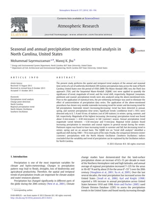
  • 9. all abrupt shift in significant trend (99% confidence interval) were found around 70s. 3.4. Regional precipitation trends Out of 249 meteorological stations studied, 3 regions of NC: mountain, piedmont, and coastal zone have 89, 82, and 78 stations, respectively. The regional trend assessment was conducted by applying the trend statistics (z-value, trend magnitude (b value), abrupt shift) on the precipitation time- series, which were the average values from stations within each region over the period 1950–2009. It is seen in Table 2 that regional precipitation trend are not significant (confidence level ≥ 95%). In annual and seasonal time series, magnitude of precipitation trend varies from −0.27 to +0.23 mm/year and from −1.13 to +0.68 mm/season, respectively. It is found in Table 2 that winter season precipi- tation is decreasing in all three regions. Annual precipitation is increasing in mountain and coastal but decreasing in piedmont region over the 60 year period. Fig. 7 shows the SQMK test results on annual and seasonal precipitation time-series for mountain, piedmont and coastal regions. Significant abrupt precipitation shifts are not detected in annual and seasonal scale precipitation, except for the coastal (mountain) region in spring (winter and summer) season. Overall, regional precipitation trend decreases statewide in annual time series. In summer, almost all 3 regions show the decreasing precipitation trend from the period of around 1960 to 2000. It seems that statewide summer precipitation trend increases in last decade. Statewide mild temporal precipitation trend increment occurs in fall season. The winter and spring seasons show no general temporal precipitation trend shift. However, statewide decreases trend detected in last decades in winter season. 3.5. Comparison of precipitation trend with NAO (North Atlantic Oscillation) index and SO (Southern Oscillation) index The NAO and SO are the primary modes of the climate variability occurring in the northern hemisphere. NAO positive (negative) phase is associated with a stronger (weaker) north– south pressure gradient between the sub-tropical high and the Icelandic low (Durkee et al., 2008). Whereas, SO is an oscillation in surface air pressure between the tropical eastern and the western Pacific Ocean waters. The strength of the SO is measured by the Southern Oscillation Index (SOI). The SOI is computed from fluctuations in the surface air pressure difference between Tahiti and Darwin, Australia (Kurtzman and Scanlon, 2007). Previous researchers anticipated the strong relationship between precipitation and Oscillation (i.e. NAO, SO) over northern hemisphere/eastern United States/southeastern United States (Durkee et al., 2008; Hurrell, 1995; Kurtzman and Scanlon, 2007). Here we compare winter (summer) precipitation with the NAO (SO) indices using 10-year moving average data (Fig. 8a and b). NAO and SO monthly data sets are collected from the Climate Prediction Center/National Oceanic and Atmospheric Administration (CPC, 2013). Monthly data were averaging out to generate the seasonal data series. Based on the coefficient of correlation (Rwinter-NAO = 0.37 and Rsummer-SOI = 0.35) and visual observation of the raw datasets of seasonal precipitation and NAO, SO indices; winter (summer) precipitation with the NAO (SO) indices was selected for the discussion in this section. Three time periods 1972–1984, 1989–1998 and 1998–2009 (Fig. 8a) were found to have similar phase of winter average precipitation with the winter NAO indices. Durkee et al. (2008) found significant increase in the occurrence of rainfall observations during positive NAO phases in the eastern U.S. Winter average precipitation increases with the increment of positive NAO index in the period of 1989–1998. Similarly, two time periods of 1967–1979 and 1985–1998 (Fig. 8b) found similar pattern of summer average precipitation with the summer ENSO indices. Kurtzman and Scanlon (2007) found varying significance level (0.05–0.001) correlation of summer precipitation with SOI over the state of North Carolina in their southern United Sates study. This section discusses the relational pattern of winter and summer precipitation trends with the NAO and SOI. However, the predictability of precipitation pattern with the long term climate variability is still an undergoing research. 4. Summary and Conclusion This paper analyzes the behavior of annual and seasonal precipitations in the state of North Carolina looking for trend in long historical (1950–2009) data series. Denser observation data (1 per 548km2 ) totaling 249 meteorological stations were applied to the non-parametric Mann–Kendall test, the Theil– Sen approach and the Sequential Mann–Kendall test to investigate the precipitation trends. MK test, TSA method, and SQMK test were applied for significant trend detection, magnitude of trend, and precipitation trends shift analysis, respectively. Three distinct region (mountain, piedmont, and coastal) precipitation trends were also analyzed based on the above tests. A pre-whitening technique was applied to pre- process the data series prior to the application of the MK test and the TSA method, in order to reduce the serial correlation in long time series, as well as its effects on trends. Table 2 Results of the statistical tests for regional (mountain, piedmont and coastal) precipitation trend of annual and seasonal time scale over the period 1950–2009. Mountain Piedmont Coastal Season/Year Z b Z b Z b Winter −1.0651 −1.1292 −0.8228 −0.4924 −0.7207 −0.5361 Spring 0.5549 0.4472 −0.4783 −0.1897 0.3635 0.2433 Summer 0.6952 0.4773 0.0702 0.0407 0.0191 0.0138 Fall 0.3253 0.1841 1.0141 0.4679 1.1799 0.6846 Annual 0.1212 0.2465 −0.1594 −0.272 0.236 0.2289 Z: Statistics of the Mann–Kendall test, b: Slope from Theil–Sen-approach (mm/season or year). 191 M. Sayemuzzaman, M.K. Jha / Atmospheric Research 137 (2014) 183–194
  • 10. Almost equal nos. of stations were showing positive and negative trends in annual time series. Among the positive (negative) trends, seven (three) significant trends were observed at the 95% and 99% confidence levels. The range of magnitude of annual precipitation trends varied from (−) 5.50 to (+) 9 mm/year. The spatial distribution of the annual precipitation trends indicated that the significant positive (negative) trends mostly happened in the south-east (mid and west) part of North Carolina. There is no single positive significant trend station found in piedmont zone. Most of Fig. 7. Graphical representation of the forward series u (d) and the backward series u′ (d) of the Sequential Mann–Kendall (SQMK) test for annual and seasonal precipitation at the 3 regions (mountain, piedmont and coastal) of North Carolina. 192 M. Sayemuzzaman, M.K. Jha / Atmospheric Research 137 (2014) 183–194
  • 11. the stations precipitation shift occurred around 1970 either positive or negative. Notable significant precipitation trend shift (either increasing or decreasing) was not detected in regional trend shift analysis. The analysis of the seasonal precipitation time series showed a mix of positive and negative trends. In winter the majority of the stations (229 out of 249) show the negative trend whereas in fall, 202 positive trend stations found. In summer positive (negative) trends were found in (92) 155 stations. This paper develops for the first time a full picture of recent precipitation trends with the denser gauging stations data across the state of North Carolina, which should be of interest to future agriculture and water resource management personnel. This study also found some correlations between North Atlantic Fig. 8. (a) 10-Year moving average of winter average precipitation and winter NAO index and (b) 10-year moving average of summer average precipitation and summer SOI. 193 M. Sayemuzzaman, M.K. Jha / Atmospheric Research 137 (2014) 183–194
  • 12. Oscillation (Southern Oscillation) indices with the winter (summer) precipitations. However, it is still unclear whether this trend change is either due to the Multi-decadal Natural Oscillation or the anthropogenic effects, such as: population change and land cover land use change or due to the greenhouse gas alteration effects, which will be the future research interests. Other different test results can also be comparable with the finding trend in this study might be an interesting inclusion with the future studies. Acknowledgements M. Sayemuzzaman like to express his special gratitude to Dr. Keith A. Schimmel, Chair in Energy and Environmental System Department for his all aspects supports. Authors also like to thank the two anonymous reviewer for their suggestion to improve the contents of this paper. References Boyles, P.R., Raman, S., 2003. Analysis of climate trends in North Carolina (1949–1998). Environ. Int. 29, 263–275. Boyles, R.P., Holder, C., Raman, S., 2004. North Carolina climate: a summary of climate normals and averages at 18 agricultural research stations. Technical Bulletin, 322. North Carolina Agricultural Research Service. Costa, A.C., Soares, A., 2009. Homogenization of climate data: review and new perspectives using geostatistics. Math. Geosci. 41, 291–305. CPC, 2013. North Atlantic Oscillation (NAO): Climate Prediction Center (CPC), National Oceanic and Atmospheric Administration (NOAA). http://www.cpc.ncep.noaa.gov/products/precip/CWlink/pna/nao.shtml (Available online at). Durkee, J.D., Frye, J.D., Fuhrmanny, C.M., Lacke, M.C., Jeong, H.G., Mote, T.L., 2008. Effects of the North Atlantic Oscillation on precipitation-type frequency and distribution in the eastern United States. Theor. Appl. Climatol. 94, 51–65. http://dx.doi.org/10.1007/s00704-007-0345-x. Gocic, M., Trajkovic, S., 2013. Analysis of changes in meteorological variables using Mann–Kendall and Sen's slope estimator statistical tests in Serbia. Glob. Planet. Chang. 100, 172–182. Hirsch, R.M., Slack, J.R., Smith, R.A., 1982. Techniques of trend analysis for monthly water quality data. Water Resour. Res. 18, 107–121. Houghton, J.T., Ding, Y., Griggs, D.J., Noguer, M., van der Linden, P.J., Dai, X., Maskell, K., Johnson, C.A., 2001. Climate Change 2001: The Scientific Basis. Contribution of Working Group I to the Third Assessment Report of the Intergovernmental Panel on Climate Change. Cambridge University Press, Cambridge, UK/New York, USA. Hurrell, J.W., 1995. Decadal trends in the North Atlantic Oscillation—regional temperatures and precipitation. Science 269, 676–679. Jha, M.K., Singh, A.K., 2013. Trend analysis of extreme runoff events in major river basins of Peninsular Malaysia. Int. J. Water 7 (1/2), 142–158. Jianqing, F., Qiwei, Y., 2003. Nonlinear time series: nonparametric and parametric methods. Springer Series in Statistics.0387224327. Karl, T.R., Knight, R.W., 1998. Secular trends of precipitation amount, frequency, and intensity in the United States. Bull. Am. Meteorol. Soc. 79, 231–241. Keim, B.D., Fischer, M.R., 2005. Are there spurious precipitation trends in the United States Climate Division database? Geophys. Res. Lett. 32. http://dx.doi.org/10.1029/2004GL021985 (L04702). Kendall, M.G., 1975. Rank Correlation Measures. Charles Griffin, London. Kurtzman, D., Scanlon, B.R., 2007. El Niño—Southern Oscillation and Pacific Decadal Oscillation impacts on precipitation in the southern and central United States: evaluation of spatial distribution and predictions. Water Resour. Res. 43. http://dx.doi.org/10.1029/2007WR005863 (W10427). Mann, H.B., 1945. Non-parametric tests against trend. Econometrica 13, 245–259. Martinez, J.C., Maleski, J.J., Miller, F.M., 2012. Trends in precipitation and temperature in Florida, USA. J. Hydrol. 452–453, 259–281. Modarres, R., Sarhadi, A., 2009. Rainfall trends analysis of Iran in the last half of the twentieth century. J. Geophys. Res. 114. http://dx.doi.org/10.1029/ 2008JD010707 (D03101). Modarres, R., Silva, V., 2007. Rainfall trends in arid semi-arid regions of Iran. J. Arid Environ. 70, 344–355. New, M., Todd, M., Hulme, M., Jones, P., 2001. Precipitation measurements and trends in the twentieth century. Int. J. Climatol. 21, 1899–1922. Partal, T., Kahya, E., 2006. Trend analysis in Turkish precipitation data. Hydrol. Process. 20, 2011–2026. Peterson, T.C., Easterling, D.R., Karl, T.R., Groisman, P.Y., Nicholis, N., Plummer, N., Torok, S., Auer, I., Boehm, R., Gullett, D., Vincent, L., Heino, R., Tuomenvirta, H., Mestre, O., Szentimrey, T., Salinger, J., Førland, E., Hanssen-Bauer, I., Alexandersson, H., Jones, P., Parker, D., 1998. Homogeneity adjustments of in situ atmospheric climate data: a review. Int. J. Climatol. 18, 1493–1517. Prat, O.P., Nelson, B.R., 2013. Characteristics of annual, seasonal, and diurnal precipitation in the Southeastern United States derived from long-term remotely sensed data. Atmos. Res. http://dx.doi.org/10.1016/ j.atmosres.2013.07.022 (in press). Robinson, P., 2005. North Carolina Weather and Climate. University of North Carolina Press in Association with the State Climate Office of North Carolina (Ryan Boyles, graphics). Salas, J.D., Delleur, J.W., Yevjevich, V., Lane, W.L., 1980. Applied Modelling of Hydrologic Time Series. Water Resources Publications, Littleton, Colorado. Sen, P.K., 1968. Estimates of the regression coefficient based on Kendall's tau. J. Am. Stat. Assoc. 63 (324), 1379–1389. Small, D., Islam, S., Vogel, R.M., 2006. Trends in precipitation and streamflow in the eastern US.: paradox or perception? Geophys. Res. Lett. 33. http:// dx.doi.org/10.1029/2005GL024995 (L03403). Some'e, B.S., Ezani, A., Tabari, H., 2012. Spatiotemporal trends and change point of precipitation in Iran. Atmos. Res. 113, 1–12. Sonali, P., Nagesh, K.D., 2013. Review of trend detection methods and their application to detect temperature changes in India. J. Hydrol. 476, 212–227. Tabari, H., Somee, B.S., Zadeh, M.R., 2011. Testing for long-term trends in climatic variables in Iran. Atmos. Res. 100 (1), 132–140. Theil, H., 1950. A rank-invariant method of linear and polynomial regression analysis. Proc. K. Ned. Akad. Wet. A53, 386–392. USDA-ARS, 2012. Agricultural Research Service, United States Department of Agriculture. http://www.ars.usda.gov/Research/docs.htm?docid=19440 (accessed November, 2012). von Storch, H., 1995. Misuses of statistical analysis in climate research. In: Storch, H.V., Navarra, A. (Eds.), Analysis of Climate Variability: Applications of Statistical Techniques. Springer, Berlin, pp. 11–26. Xu, Z.X., Takeuchi, K., Ishidaira, H., Li, J.Y., 2005. Long-term trend analysis for precipitation in Asia Pacific Friend river basin. Hydrol. Process. 19, 3517–3532. 194 M. Sayemuzzaman, M.K. Jha / Atmospheric Research 137 (2014) 183–194