SlideShare una empresa de Scribd logo
1 de 198
From First Principles January 2017 – R4.7
Maurice R. TREMBLAY
PART X – SUPERSTRING THEORY
A Calabi-Yau manifold is an
example of a smooth space
(i.e., it is Ricci flat – RΜΝ =0)
that represents a deformation
which, from a space-time
point of view, smooths out an
orbifold singularity (i.e., an
infinite amount of curvature
located at each of the points.)
Chapter 1
In 1964, Feynman said in his Lectures on Quantum Mechanics (Vol. III): “I think I can
safely say that nobody understands quantum mechanics.” Well, that was back in the day
when he worked on a quantum theory of gravitation (c.f., Acta Phys. Pol.) and if he were
to extend the point particle idea to that of a vibrating string and develop a theory that des-
cribes energy and matter as being composed of tiny, wiggling strands of energy that look
like strings, then surely he would say: “I think I can safely say that only Ed Witten under-
stands string theory.” So, in no way does this set of slides come close to the height of his
intellect but it is meant to provide at least some familiarity to study the more established
and serious textbooks on the subject (c.f., References) and spearhead some gifted kid!*
Forward
2
2017
MRT
As with my other work, nothing of this is new or even developed first hand and frankly
it is a rearranged compilation of various quotes from various sources (c.f., ibid) that aims
to display an abridged but yet concise and straightforward mathematicaldevelopment of
string theory and superstrings (and some compactificationas a consequence) as I have
understood it and wish it to be presented to the layman or to the inquisitive person. Now,
as a matter of convention,I have included the setting h≡c≡1 in most of the equations and
ancillary theoretical discussions and I use the summation convention that implies the
summation over any repeated indices (typically subscript-superscript) in an equation.
* In order for someone to do active string theory research today, you have to be a very smart and committed person…Seriously!
Anyhow, this is my take on string theory… It will be work in progress (in three parts
probably) for some time to come as I myself mature and develop skills to make sense of
it all. String theory is a tough subject and it does require mathematical and physical intu-
ition that is so daunting but it will be quite a challenging experience to unravel some of it!
Contents of 2-chapter PART X
2017
MRT
PART X – SUPERSTRING THEORY
A History of the Origins of String
Theories
The Classical Bosonic String
The Quantum Bosonic String
The Interacting String
Fermions in String Theories
String Quantum Numbers
Anomalies
The Heterotic String
Compactification and N=1 SUSY
Compactification and Chiral Fermions
Compactification and Symmetry
Breaking
Epilogue: Quantum Gravity
Appendix I: The Gamma Function
Appendix II: The Beta Function
Appendix III: Feynman’s Take on
Gravitation
Appendix IV: Review of Supersymmetry
“We propose that the ten-dimensional E8×E8 heterotic string is related to an eleven-dimensional theory on
the orbifold R10×S1/Z2 in the same way that the Type IIA string in ten dimensions is related to R10×S1. This
in particular determines the strong coupling behavior of the ten-dimensional E8×E8 theory. […]” Petr
Hořava and Edward Witten, Preface to their paper prescribing M-Theory for the first time (1995).
Appendix V: A Brief Review of Groups
and Forms
References
Contents
2017
MRT
PART X – SUPERSTRING THEORY
A History of the Origins of String
Theories
The Classical Bosonic String
The Quantum Bosonic String
The Interacting String
Fermions in String Theories
String Quantum Numbers
Anomalies
The Heterotic String
Compactification and N=1 SUSY
Compactification and Chiral Fermions
Compactification and Symmetry
Breaking
Epilogue: Quantum Gravity
Appendix I: The Gamma Function
Appendix II: The Beta Function
Appendix III: Feynman’s Take on
Gravitation
Appendix IV: Review of Supersymmetry
Appendix V: A Brief Review of Groups
and Forms
References
The story of the development of string theories is such a beautiful example of the
disorganized and unpredictable way in which elementary particle theory has evolved that
we cannot resist the temptation to give a brief historical (i.e., mathematical) introduction.
5
2017
MRT
A History of the Origins of String Theories
During the early 1960s, particle physics, or at least the strong-interaction sector which
was receiving the most attention, both theoretical and experimental, was dominated by
S-matrix theory. Its basic ingredients were the general properties of the scattering matrix
or S-matrix (N.B., the S-matrix elements are given by 〈 f |S|i〉 which are the probability
amplitudes for the transition between an initial state i and a final state f ) rather than
fundamental fields described by Lagrangians. The S-matrix was expected to be
determined mainly by the requirements of analyticity, crossing, and unitarity, terms
which we shall now explain.
In their seminal two-volume treatise (suitable for an ‘advanced’ graduate-level course),
M. Green,J. Schwarz and E. Witten, Superstring Theory, Vol. I - Introduction, Cambridge
University Press (1987), Section 1.1 entitledThe Early Days of Dual Models, gives a more
detailed and systematic study than the rough outline that is presented in this chapter. That
first section of their book begins with the paragraph: “In 1900, in the course of trying to fit
to experimental data, Planck wrote down his celebrated formula for blackbody radiation
(i.e., I(ν,T )=(2hν 3/c2){1/[exp(hν/kBT )−1]}). It does not usually happen in physics that an
experimental curve is directly related by a more or less intricate chain of calculations.
But blackbody radiation was a lucky exception to this rule. In fitting to experimental
curves, Planck wrote down a formula that directly led […] to the concept of the quantum.”
It is convenient to write the S-matrix as the sum:
6
2017
MRT
22
)()( dcba pppps +=+≡
AiS += 1
where 1 is the unit matrix representing processes in which the particles do not interact,
and A is the scattering amplitude. The analyticity assumption is that A must be an
analytic function of the Lorentz invariants that describe the process, with only isolated
singularities that are determined by the spinless particles (c.f., PART VIII – THE
STANDARD MODEL: Scattering Experiments):
dcba +→+
This is an analytic function of the two-independent Lorentz invariants that can be formed
from the four-momenta (i.e., pa ≡pa
µ, &c.) of the particles:
and:
22
)()( dbca ppppt −=−≡
referred to as s-channel and t-channel, respectively. The Diagram below shows the flow.
There is also u=(pa −pd)2 =(pb −pc)2. s, t, and u are the well-known Mandelstam variables.
++
↑↑↑↑
+→+ dcba
−−
↑↑↑↑
+→+ dcba
s-channel t-channel
The amplitude will contain poles corresponding to the propagators of single particles.
For example, a particle of spin J and mass M coupling to the state a+b will give a pole of
the form:
7
2017
MRT
L+
−
= 221
)(
),(
Ms
zP
ggtsA sJ
where g1 and g2 are the coupling constants (see Figure), PJ a Legendre function and zs is
the cosine of the scattering angle in the center-of-mass system. In the simple case when
the masses of the external particles are all equal to m, we readily calculate from the t-
channel process t=4m2 −2E2 +2|p|2 cosθ (c.f., op cit) that zs =1+2t/(s−4m2). The physical
region of the variables for this so-called s-channel process is given by the conditions:
04 2
≤≥ tms and
Processes giving (Left) an s-channel pole at s=M2 and (Right) a t-channel pole at t =M2.
s
t
Mg1 g2
a
b
c
d
s
t
M
g′1
g′2
a
b
c
d
Crossing is the assumption that the same scattering amplitude, analytically continued
to appropriate regions of the variables, also describes the crossed processes:
8
2017
MRT
04 2
≤≥ smt and
The physical region for the first of these (called the t-channel process because in this
case t≡(pa −pc)2 =(pb −pd)2 gives the total center-of-mass energy) is:
bcdadbca +→++→+ and
Crossing requires that the amplitude has poles, analogous to those of A(s,t) above:
L+
−
′′= 221
)(
),(
Mt
zP
ggtsA tJ
The other main ingredient of S-matrix theory is that S is unitary:
1=SS†
in any physical region for any given process. This ensures the conservation of
probability (i.e., that the sum over all the possible things that can happen is unity or
always 100% every time, if you wish). We note that the sum over all possible
intermediate states implied in the matrix multiplication S†S=1 above automatically
couples together an infinite sequence of possible processes. Also, since only those
states that are energetically possible can contribute, unitarity requires the existence
of new singularities at each new threshold. They are branch points, the first of which
occurs at s=4m2 in our example above. More generally, they arise at values of s equal
to the square of the sum of the masses of the particles in the intermediate state.
In order to make calculations in S-matrix theory, use was made of various pole
approximations. Clearly, in the neighborhood of a pole (e.g., s≈M2), that pole will
dominate the amplitude. Because of the large number of resonances, it seemed
reasonable to guess that a sum over such resonances:
9
2017
MRT
∑ −
=
i i
sJ
ii
Ms
zP
ggtsA i
221
)(
),(
might be a fair approximation to the amplitude in the physical s-channel region. Note that
the above lowest s-channel threshold the states are unstable, so the masses are
complex, Mi →Mi −½iΓi , the imaginary part being the decay width Γi.
The t-channel poles, on the other hand, give the forces that dominate forward
scattering (i.e., zs ≅1 so t is near zero). However, a t-channel pole corresponding to a
particle of high spin would give an unacceptable contribution at high s, since it behaves
like:
JJ
ttJ
tJ
szzPtsA
Mt
zP
ggtsA ~~)(~),(
)(
),( 221 →+
−
′′= L
at fixed t whereas unitarity can be shown to allow only amplitudes growing no faster than
s.
Now, in order to understand the significance of such t-channel poles for the s-channel
scattering process, it is necessary to make a partial-wave expansion in the t-channel
and to define an analytic continuation of the partial-wave amplitude to complex values of
the angular momentum J. The poles then occur along so called Regge trajectories:
10
The solutions of this equation for integer values of J give the mass-squared of the
particle, the value of J being its spin.
A typical Regge trajectory. This trajectory
connects a particle of mass m1
2 and spin-
1 and a particle of mass m2
2 and spin-2.
There is also a spin-0 tachyon state ( ) of
negative [mass]2, which must be removed
by having zero residue.
2017
MRT
For example, a nonrelativistic three dimensional harmonic
oscillator of classical frequency ω has the energy eigenvalues:






++ω=





+ω=
2
3
2
2
3
, JnnE rJn hh
where nr is the radial quantum number and J is the orbital angular
momentum. Although J is quantized (J=1,2,…) this equation can
be regarded as giving the mass of the bound states Mn,J (=En,J)
as a function of J. We can invert it to write the Regge trajectory:
)(
2
3
2 2
Mn
M
J r α≡−−
ω
=
h
More generally, a Regge trajectory connects particles with the
same internal quantum numbers but different spins (see Figure).
)(sJ α=
s
α(s)
m1
2 m2
2
1
2
)(sJ α=
−m0
2
0
The t-channel partial wave expansion does not converge in the s-channel physical
region, but it is possible to replace the sum over integer J by a contour integral in the
complex J plane which is well defined everywhere. For high s, this integral is dominated
by the rightmost singularities in the J plane, which under suitable assumptions, will be
Regge poles. We therefore obtain an approximation of the form:
11
2017
MRT
∑i
t
i
i
sttsA )(
)(~),( α
β
showing that the large s amplitude at fixed t is dominated by the leading Regge
trajectories (i.e., those with the largest αi(t)). Thus, the high-energy behavior of a given
s-channel process is determined by the particles that can be exchanged in the t-channel
(i.e., those with the t-channel quantum numbers).
The equations A(s,t)=Σigi1gi2[Pzi
(zs)/(s−Mi
2)] and A(s,t)~Σi βi(t)sαi(t) above are
approximate expressions for the scattering amplitude in terms of the s- and t-channel
poles, respectively. They have very different analytic forms but, if both are reasonable
approximations to the amplitude in part of the physical region, they must be
approximately equal to each other, at least in some average sense. This is the
assumption of duality (i.e., the resonances approximately equal Regge poles) for
hadron scattering:
∑∑ ≅
− i
t
i
i i
sJ
ii
ii
st
Ms
zP
gg )(
221 )(
)( α
β
In 1968, Veneziano proposed the following toy model of a scattering amplitude A that
satisfies duality:
12
Regge trajectories of the Veneziano
model (with scattering amplitude: A(s,t)=
Γ[−α(s)]Γ[−α(t)]/Γ[−α(s)−α(t)].
2017
MRT
It has s- and t-channel poles corresponding to particles of all
spins J=0,1,2,…, whose masses are given by the solutions of:
JM =)( 2
α
(see Figure), because Γ(x) has poles at x= 0,−1,−2,…. Also,
since:
ba
x
x
bx
ax −
∞→
 →
+Γ
+Γ
)(
)(
the Veneziano amplitude also has the Regge asymptotic behavior
of A(s,t)~Σi βi(t)sαi(t) as s→∞ at fixed t. It can be shown that it fully
satisfies the duality hypothesis in the sense that the sum over the
infinite set of s-channel poles reproduces this Regge behavior.
∫
−−−−
−=−−=
−−Γ
−Γ−Γ
=
1
0
1)(1)(
)1()](),([
)]()([
)]([)]([
),( ts
xxxdtsB
ts
ts
tsA αα
αα
αα
αα
where s and t are the Mandelstam variables from above, B is the combination of Euler
Gamma functions, Γ, known as the Beta function. This expression is clearly crossing
symmetric under s↔t and, provided the Regge trajectory function α(s) is linear:
ss ααα ′+= )0()(
where α′ is the slope and α(0) the intercept of the trajectory.
s
α(s)
1
2
3 sd
sd )(α
α =′
)0(α
Generalization to more complicated amplitudes, such as many-particle production
processes, we soon made and, for a time, there was much activity trying to fit such dual-
model Veneziano amplitudes to experimental data. Even a year later, in 1969, Virasoro
generalized Veneziano amplitude by using the four-point function:
13
2017
MRT
The next step was to try to deduce these dual-model amplitudes from some underlying
dynamics, and the key here was the realization that the spectrum of states is that of a
relativistic string. It was then found that the interaction of two open strings led
automatically to the existence of closed strings. The dual-string model required a new
trajectory to have a slope α ′/2, in rough agreement with experiment.
However, a major problem is that the particle poles are all on the real axis, whereas in
reality they should lie below this axis if they are to correspond to unstable particles (i.e.,
if their masses are above the physical threshold). Attempts to correct this by putting
branch points into the function α(s) are not successful because they destroy the linearity
that is essential to achieve the other satisfactory properties of the model. Thus, dual
models came to be seen as just the first-order term in some type of expansion, in which
the higher-order terms would ensure unitarity and push the poles off the real axis.
)](½)(½[)](½)(½[)](½)(½[
)](½[)](½[)](½[
),(
utusts
uts
tsA
αααααα
ααα
−−Γ−−Γ−−Γ
−Γ−Γ−Γ
=
In spite of interesting work on a possible dynamical theory underlying dual models,
and some success with its phenomenology, interest in the dual model of hadron declined
during the early 1970s. Serious obstacles were that self-consistency required that the
ground state of the closed string must have spin-2, rather than the spin-1 required for the
Pomeron (i.e., a particle that was invented to explain the behavior of elastic-scattering
cross sections), and that the models are only fully satisfactory in higher-dimensional
spaces. Also, the clear evidence for a parton-like behavior in deep inelastic scattering
suggested the existence of pointlike constituents within hadrons and led to the
reinstatement of field theory, with quarks and gluons as the new fundamental fields. The
idea that hadrons are a self-consistent set of states uniquely determined just by the
postulates of S-matrix theory (i.e., the bootstrap hypothesis) became untenable.
14
2017
MRT
The dual model, however, lived on. It survived by abandoning hadron physics and
becoming instead a candidate theory of the fundamental particles. All of this stemmed
from a suggestion by Scherk and Schwarz (1974) that the spin-2 value for the closed
string ground state should be taken as an indication that the theory contains gravity, and
that the slope α ′ should be taken as O(EP
−2) (EP being the Planck energy), so that only
the ground states of the strings with mass<<MP ≡EP /c2 are observed in normal physics.
Instead their role is to improve the chance of obtaining a finite theory of all interactions,
including gravity, by modifying the very short-distance behavior. However, higher dimen-
sionality is required and it is hoped that a suitable compactification scheme, ideally one
forced by the theory rather than selected by us to produce the required results, will
lead to something like the standard supersymmetry (SUSY) model for E<<EP.
The ultraviolet (i.e., large-momentum or short-distance) infinities of field theory (i.e., the
realm of Renormalization Theory) have their origin in the supposed pointlike nature of
elementary particles, and are indeed related to the well-known divergence of the
electromagnetic self-energy of a classical point charge. It is, therefore, natural to wonder
whether the idea that elementary particles as points should be instead considered as
extended objects. (N.B., We are not thinking of extension in the sense that the proton,
for example, has finite size owing to the spatial distribution of its pointlike constituents –
the quarks. Rather, we are introducing size as an intrinsic property of even elementary
objects).
15
The Classical Bosonic String
A particle trajectory xµ =xµ(τ) between τ1
and τ2.
2017
MRT
We recall from Sp=−m ∫dτ √(gµν xµxν ) of the PART IX – SUPER-
SYMMETRY: The Newtonian Limit chapter that the action for
such a particle is proportional to path length (see Figure):
∫ ⋅−= xxdmSp &&τ
where x ≡dx/dτ (N.B., x is shorthand for xµ) and τ is the para-
meter used to label positions on the trajectory. Minimization of
this action with respect to variations in xµ(τ) yields ∂[xµ/√(x⋅x)]/∂τ
=0. If we choose τ as the proper time, this gives the expected
result (c.f., xρ+Γρ
µν xµ xν =0 with no gravitational fields – i.e., gµν
=ηµν so Γρ
µν =0). The momentum conjugate to xµ is given by:
⋅⋅⋅⋅ ⋅⋅⋅⋅
⋅⋅⋅⋅
from which we obtain (N.B., p is also shorthand for pµ):
⋅⋅⋅⋅ ⋅⋅⋅⋅ ⋅⋅⋅⋅
⋅⋅⋅⋅⋅⋅⋅⋅⋅⋅⋅⋅⋅⋅⋅⋅
xx
xm
x
L
p
&&
&
& ⋅
==
µ
µ
µ
δ
δ
2
mpp =⋅
x2 x0
τ1
τ2
x1
We now generalize these results to a one-dimensional extended object (i.e., a string).
We require the string to have a finite length, so it can be either an open string, with two
free ends, or a closed string, with no free ends but loops around itself. The trajectories
followed by such strings are two dimensional surfaces in space-time (see Figure).
16
Parameters τ and σ label the time and space directions, respectively, so that σ1 labels a particular point
on the string. (Left) A typical trajectory for an open string. (Right) A typical trajectory for a closed string.
2017
MRT
These surfaces can be labeled by two parameters τ and σ such that the space-time
coordinate is:
x2
x1
x0
τ1
τ2
σ1
x2
x1
x0
τ1
τ2
σ1
xµ(τ,σ)xµ(τ,σ)
where µ =0,1,…,(D −1) with D being the dimension (e.g., D=4 is 4D). We will normally
think of τ as labeling the time and σ the space direction. For the open string, we choose
0≤σ ≤π and, correspondingly, for the closed string we impose that xµ(τ,σ +π)=xµ(τ,σ).
),( στµµ
xx =
0 ≤σ ≤π xµ(τ,σ +π)=xµ(τ,σ)
The obvious generalization of the path length Sp =−m∫dτ √(x⋅x) above is to take the
action of a string to be proportional to the area of the surface mapped out as it moves
between τ1 and τ2. Thus, we put, where we reinsert the constants h and c for clarity:
17
2017
MRT
where x′≡∂x/∂σ and where α ′ is a parameter that will later turn out to be the slope of
the Regge trajectory associated with the string. Alternatively, (2πα ′hc)−1 represents the
tension To in the string. Up to factors of h and c, the string length is the square root of α ′:
∫=′⋅′⋅−′⋅
′π
−=
2
1
1
))(()(
2
1 2
τ
τ
τσ
α
ddL
c
Sxxxxxx
c
L and&&&
h
⋅⋅⋅⋅ ⋅⋅⋅⋅
The classical equation of motion for the closed string, obtained by minimizing S, is
(c.f., the Euler-Lagrange equation of PART VIII – THE STANDARD MODEL: Field
Equations):
0=







′∂
∂
+







∂
∂
µµ
δ
δ
σδ
δ
τ x
L
x
L
&
or, explicitly:
0
)()()()(
=







 ′⋅−′⋅
∂
∂
+







 ′⋅′−′′⋅
∂
∂
L
xxxxxx
L
xxxxxx µµµµ
στ
&&&&&&
This is a very complicated equation of motion! (N.B., L→√[(x⋅x′)2 −(x⋅x)(x′⋅x′)]!)
oπ2
1
T
cs
α
α
′
=′= hl
⋅⋅⋅⋅ ⋅⋅⋅⋅ ⋅⋅⋅⋅
This last equation above can be simplified if we use the freedom of reparametrization
invariance to require that the σ and τ directions be orthogonal (see Figure):
18
2017
MRT
0=′⋅ xx&
and also scale σ,τ so that the distance moved when σ changes by dσ is equal to that
moved when τ changes by dτ =dσ. Recalling that these distances are spacelike and
timelike, respectively, we can write this condition as:
0=′⋅′+⋅ xxxx &&
Illustrating orthonormal coordinates on the
open string trajectory.
For some purposes it is useful to remove the remaining
freedom in τ and σ by putting:
)()constant( µ
µτ xn=
where n is a constant vector. One particular choice of n, in which
it has the components:
so it is on the light-cone:
]1...,,0,0,1[
2
1
−=µn
When these two last conditions above are satisfied, we are said to be using an
orthonormal or conformal gauge. In such a gauge, the equation of motion above
becomes the familiar wave equation:
µµ
xx ′′=&&
leads to the so-called light-cone or transverse gauge.
0=⋅nn
τ1
σ1 σ2
σ3
τ2
τ3
With xµ =x″µ above, we can write the general solution for a closed string in the form:
19
2017
MRT
and:
where XL
µ, XR
µ are arbitrary, twice-differentiable, functions that represent waves traveling
in opposite directions ( left and right , respectively) around the closed string. The
boundary condition xµ(τ,σ +π)=xµ(τ,σ) above implies that they can be written in the
form:
)()(),( στστστ µµµ
−++= RL XXx
⋅⋅⋅⋅⋅⋅⋅⋅
∑≠
+−
+++=
′ 0
)(2
0 e
1
2
)(
2
1
2
1
n
niL
nL
n
i
qX στµµµµ
αστα
α
∑≠
−−
+−+=
′ 0
)(2
0 e
1
2
)(
2
1
2
1
n
niR
nR
n
i
qX στµµµµ
αστα
α
where qµ, α0
µ, and (α µ)n
L,R are all Lorentz vectors, with qµ and α0
µ being real (N.B.,
these are the center-of-mass position and momentum of the string, respectively) and
with:
*)( ,, RL
n
RL
n −= αα
(N.B., The Fourier decompositions XL
µ/√(2α′) and XR
µ/√(2α′) above will be essential to
quantize the string. Then the αs will have an interpretation as creation/annihilation
operators and the inclusion of the factors √(2α ′) and 1/n will give an appropriate
normalization to the αn parameters.)
The apparent simplicity of the solution xµ(τ,σ)= XL
µ(τ +σ)+XR
µ(τ −σ) is spoilt by the
above constraints (i.e., x⋅x′=0 and x⋅x+ x′⋅x′=0) which become:
20
2017
MRT
must be zero, that is:
Using XL,R
µ/√(2α′) above, these equations imply that the so-called Virasoro generators
defined by:
0=⋅=⋅ RRLL XXXX &&&&
⋅⋅⋅⋅ ⋅⋅⋅⋅ ⋅⋅⋅⋅
∑
+∞
−∞=
−⋅−≡
k
L
kn
L
k
L
nL αα
2
1
The closed string that we have considered here is oriented in the sense that changing
σ →−σ generally changes the solution. It is possible to consider an unoriented closed
string on which we impose invariance under σ →−σ. Clearly, from xµ(τ,σ)= XL
µ(τ +σ)+
XR
µ(τ −σ) above, this requires:
( )stringclosedunorientedµµ
RL XX =
( )nLL R
n
L
n 0 allfor==
∑
+∞
−∞=
−⋅−≡
k
R
kn
R
k
R
nL αα
2
1
and
The open string can be treated in a similar way, but a new problem arises: minimiza-
tion of the action does not lead to the Euler-Lagrange equation of motion above because
of the contributions of boundary terms at σ =0 and π. These stem from the integration by
parts. In order to remove the boundary terms, we require that open strings satisfy the
boundary conditions:
21
2017
MRT
Given x′µ(τ,0)=x′µ(τ,π)=0 above we can proceed as before, except that for open
strings we need the standing-wave solution:
Equation x⋅x+ x′⋅x′=0 above then implies that x⋅x=0 at σ =0 and σ =π (i.e., that the ends
of the string move with the velocity of light!)
0),()0,( =π′=′ ττ µµ
xx
⋅⋅⋅⋅ ⋅⋅⋅⋅ ⋅ ⋅
)cos(e
1
),(
2
1
0
0 σαταστ
α
τµµµµ
∑≠
−
++=
′ n
ni
n n
n
iqx
where again qµ and α0
µ are real and:
*)( µµ
αα nn −=
As before, the constraint equations (i.e., x⋅x′=0 and x⋅x+ x′⋅x′=0) imply that:⋅⋅⋅⋅ ⋅⋅⋅⋅ ⋅⋅⋅⋅
0
2
1
=⋅−≡ ∑
+∞
−∞=
−
k
knknL αα
It is possible to simplify the constrain equations if we work in the light-cone gauge,
defined by τ =(constant)(nµ xµ) and nµ=(1/√2)[1,0,0,…,−1] above. For this purpose we
introduce D-dimensional light-cone coordinates:
22
2017
MRT
where bold-face quantities are vectors in the (D−2)-dimensional transverse space, with
components x1, x2, …, xD−2. Also, from τ =(constant)(nµ xµ) and nµ=(1/√2)[1,0,0,…,−1]
above:
which, to put things into perspective, reduces to the x± ≡(1/√2)(x0 ±x3) and x1, x2 light-
cone coordinates (x1, x2 being transverse coordinates) when D=4 is taken to be physical
space-time. Then any vectors x and y satisfy:





±≡
−
−±
221
10
,,,
)(
2
1
D
D
xxx
xxx
K
yx ⋅⋅⋅⋅−=⋅ −+
xxyx
+
= x)constant(τ
and hence in xµ(τ,σ)/√(2α ′) above, q+ and αn
+ (n≠0) are zero. Thus, the constraint Ln ≡
−½Σkαk ⋅αn−k =0 above becomes an equation for αn
−:
∑
+∞
−∞=
−+
−
=
k
knkn αααα⋅⋅⋅⋅αααα
0
1
α
α
showing that the only degrees of freedom are α0
+, q−, and the transverse modes ααααk.
Similarly, for the closed string, τ =(constant)x+ above (N.B., recall that we also defined
x± ≡(1/√2)(x0 ±x3) above) implies that (α n
+)L,R =0 (for all n≠0), so the constraints give:
23
2017
MRT
in the conformal gauge. The total momentum of the string is obtained by integrating pµ
over the whole string:
We calculate the momentum as for a point particle:
∑ −+
−
=
k
L
kn
L
k
L
n αααα⋅⋅⋅⋅αααα
0
1
)(
α
α
αδ
δ µ
µ
µ
′π
==
2
x
x
L
p
&
&
µµµµ
α
α
αα
α
σ 00
2/1
0
2
2)2(
2
1
′
=π′
′π
== ∫
π
pdP
for the closed string, and:
µµµ
α
α
α
α 00
2
12
2
1
′
=
′
=P
for the open string.
showing that the only degrees of freedom are α0
+, q−, and the transverse modes (ααααk)L,R.
∑ −+
−
=
k
R
kn
R
k
R
n αααα⋅⋅⋅⋅αααα
0
1
)(
α
α
and
( )movers
( )movers
Left
Right
These equations determine the mass of the string. For the closed string we have:
24
2017
MRT
In the light-cone gauge, these last two equations for the M2 of closed and open strings
become:
where to obtain the last line we have used the zero-frequency constraints Ln
L=Ln
R =0 (for
all n) above (N.B., Ln
L=Ln
R =0 also implies that the L and R contributions to the mass are
identical). For the open string we find, similarly:
∑
∞
=
−− ⋅+⋅
′
−=⋅
′
=⋅=
1
00
2
)(
22
n
R
n
R
n
L
n
L
nPPM αααα
α
αα
α
∑
∞
=
− ⋅
′
−=⋅
′
=
1
00
2 1
2
1
n
nnM αα
α
αα
α
and:
( )closed∑
∞
=
−− +
′
=
1
2
)(
2
n
R
n
R
n
L
n
L
nM αααα⋅⋅⋅⋅αααααααα⋅⋅⋅⋅αααα
α
( )open∑
∞
=
−
′
=
1
2 1
n
nnM αααα⋅⋅⋅⋅αααα
α
respectively.
Before we proceed to quantize the string, it is of interest to introduce an equivalent
classical model defined by the action (c.f., S= ∫τ Ldσ dτ above):
25
2017
MRT
where R(D=2)(hab)≡habRab
(D=2) is the scalar curvature obtained from hab and where Rab
(D=2)=
∂b Γc
ac −∂c Γc
ab −Γc
ab Γd
cd +Γc
ad Γd
bc with Γc
ab=½hcd (∂a hbd +∂b had − ∂d hab ). However, in two
dimensions, such a term is a constant that does not affect the dynamics!
where h=−det(hab) with hab the metric on the two-dimensional world-sheet of the string.
The indices a,b take values 0,1 (N.B., ξ 0, ξ 1 here play the roles of τ,σ used earlier). We
can think of the action S above as describing a set of D=2 scalar fields xµ(ξ 0,ξ 1) on a
two-dimensional space-time, with background metric hab (i.e., the usual space-time
variables have become scalar fields). Such an interpretation suggests several possible
generalizations. One fairly obvious possibility is to add to S above the action of Einstein’s
gravity on the two-dimensional world-sheet:
ba
ab xx
hhddS
ξξ
ξξ
α ∂
∂
⋅
∂
∂
′π
−= ∫
10
4
1
)()2(10)2( abDD
hRhddS ==
∫= ξξ
The equivalence of S= ∫τ Ldσ dτ and S above, as classical theories, can be demons-
trated by finding the Euler-Lagrange equation corresponding to variations in hab, solving
it, and using the solution to eliminate hab from S above, thereby recovering the action S=
∫τ Ldσ dτ. However, such an equivalence does not in general hold in quantum theory
because of the quantum fluctuations about the minimum solution for hab.
More can be said about the nature of these fluctuations by noting that hab, being sym-
metric, is defined by three independent functions of ξ 0,ξ 1. The freedom to reparametrize
(i.e., reparametrization invariance) allows us to introduce two new arbitrary functions:
26
2017
MRT
and so the only remaining degree of freedom is the scale (or conformal) factor φ(ξ 0,ξ 1).
When we insert this hab into S above the factor φ clearly cancels and so plays no role in
the classical equations. In fact, with hab above, we can write S as:*
for a=1,2, which can be chosen so that hab has the form:
),( 10
ξξξξ aa
′=′
baba
h ηξξφξξφ ),(
10
01
),( 1010
=





−
=
ba
ab xx
ddS
ξξ
ηξξ
α ∂
∂
⋅
∂
∂
′π
−= ∫
10
4
1
* Green, Schwarz & Witten (c.f., § 1.3.3), in their notation, use, hαβ =ηαβ expφ where expφ is an unknown conformal gauge. Their
free field action reduces to S=−(T/2)∫dσ 2ηµνηαβ ∂α Xµ ∂β Xν (with dσ 2 ≡dτ dσ and Xµ=Xµ(τ,σ) is their label for string position).
In quantum theory it is necessary to do a path integral over all metrics and all
trajectories x(ξ a). This requires us to define suitable weights for the path integrals and to
remove the divergences that arise. A. M. Polyakov (1981) showed that S above is
equivalent to S= ∫τ Ldσ dτ if, and only if, the dimension of space-time is D=26! This
cancellation of divergences, which seems to be essential for a consistent string theory, is
referred to as the cancellation of the conformal anomaly where Lorentz invariance is
only established in the critical dimension for bosonic strings:
In the above discussion we have implicitly assumed that the background (i.e., D=26)
space-time is flat (i.e., gµν =ηµν ) – we have ignored gravity! Since the string automati-
cally contains gravity, this is inconsistent. The correct requirement for conformal
invariance to hold is that the background metric should satisfy an equation that, in lowest
order, reduces to Einstein’s equation Rµν −½Rgµν=−κ 2Tµν (c.f., PART IX – SUPERSYM-
METRY: The Inclusion of Matter or Appendix III: Feynman’s Take on Gravitation for a
field theory derivation of gravitation).
27
2017
MRT
26=D
The quantization of a classical system is not always a uniquely defined procedure. The
classical limit can be regarded as the first term of an expansion in powers of h and there
is clearly an infinite number of possible expansions that have the same zeroth-order
limit. Several methods of quantizing the classical string, based on the analogy with point-
particle models, have been used, and the results agree provided that certain consistency
conditions are satisfied.
28
2017
MRT
Here we use the canonical quantization method (as opposed to light-cone gauge
quantization) in which we regard xµ(τ,σ) and its conjugate momentum pµ(τ,σ)=xµ/2πα′
as operators that satisfy the equal-time commutation relation:
The Quantum Bosonic String
⋅⋅⋅⋅
)()],(),,([ σσδστστ νµνµ
′−−=′ gipx
Using the Fourier expansion xµ(τ,σ)/√(2α′)=qµ +α0
µ +iΣn≠0(1/n)αn
µ exp(−inτ)cos(nσ) for
the open string, we see that this relation requires:
νµνµ
α giq −=],[ 0
all the other commutators being zero. Using αm
µ =(α−m
µ)† we can replace [αm
µ †,αn
ν]
above by:
νµνµ
δαα gn nmnm =],[ †
which shows that we can regard αn and its adjoint αn
†, for positive n, as annihilation
and creation operators, respectively.
and:
νµνµ
δαα gm mnnm 0,],[ +−=
We shall now impose the constraint Ln ≡−½Σk=±∞ αk ⋅αn−k =0 of the The Classical
Bosonic String chapter by working in the light-cone gauge (N.B., there is also the
Lorentz covariant quantization approach which will not be used here). Since there is no
longitudinal motion, this means that only the transverse operators αn
ν used in the
canonical quantization method (where ν =1,2,…,D−2) represent independent degrees of
freedom, and for these:
29
2017
MRT
assuming the background is flat (i.e., gµν =ηµν). It should be noted, however, that this
choice of gauge breaks the explicit Lorentz invariance of the theory, which is the source
of a difficulty that we shall encounter below.
ˆ
ˆ
νµνµ
δδαα ˆˆˆ†ˆ
],[ nmnm n−=
The vacuum state, |0〉, can be defined as the eigenstate of all the annihilation
operators, αn
µ (n positive), that has zero eigenvalues:ˆ
( )...,2,1,000ˆ
== nn
µ
α
Other states of the system can be obtained by acting on |0〉 with the creation operators
α−1
ν, α−2
ν, &c.ˆ ˆ
We can calculate the mass of the resulting states by using the mass operators given
by M2 =(1/2α′)α0 ⋅α0 of the The Classical Bosonic String chapter. However, when we
relate this to the αn operators by means of the constraints (i.e., to obtain the analog of
M2 =−(1/α′)Σnα−n⋅αn), we meet a new problem. The operators must be normal ordered
(i.e., all the annihilation operators must be placed to the right of all the creation
operators). Since the order is irrelevant for classical quantities, and each change of
order introduces a constant as in [αm
µ†,αn
ν ]=−nδmnδ µν above, the reordering required to
produce the quantized expression introduces an arbitrary constant. Thus, instead of M2 =
−(1/α′)Σnα−n⋅αn of the The Classical Bosonic String chapter we write:
30
2017
MRT
where the number operator N is defined to be:
)]0([
12
α
α
−
′
= NM
∑
∞
=
−=
1n
nnN αααα⋅⋅⋅⋅αααα
in the light-cone gauge, and where we have called the unknown constant α(0). The
reason for this choice is that, if we rewrite M2 =(1/α′)[N−α(0)] above in the form:
2
)0( MN αα ′+=
it becomes reminiscent of the linear Regge trajectory of slope α ′ and intercept α(0)
as in α(s)=α(0)+α ′s of the A History of the Origins of String Theories chapter, if N is
interpreted as the angular momentum.
ˆˆ ˆˆ
In order to study the angular momenta of the states, we need the angular-momentum
operators:
31
2017
MRT
which are generalizations of the angular momentum in three dimensions discussed in
PART IX – SUPERSYMMETRY: The SUSY Algebra chapter or Appendix IV: Review of
Supersymmetry. In the The Classical Bosonic String chapter,we used the expansion
[1/√(2α′)]xµ(τ,σ)=qµ +αm
µτ +iΣn≠0(1/n)αn
µ ⋅exp(−inτ)cos(nσ) and this becomes:
∫ −=
π
0
)( µννµµν
σ pxpxdM
∑
∞
=
−− −
+−=
1
00
)(
)(
n
nnnn
n
iqqM
µννµ
µννµµν αααα
αα
We can use this expression to calculate explicitly the commutation relations of the
different components of Mµν. These do not turn out to be exactly what one would expect
for angular momentum. In particular, when we use (±) light-cone gauge coordinates x± ≡
(1/√2)(x0 ± xD−1), and calculate the commutation relations between the components M−µ
(where µ are the transverse coordinates as in [αm
µ†,αn
ν ]=−nδmnδ µν above), we obtain:ˆˆ ˆˆ
ˆ
ˆ
∑
∞
=
−−+
−−
−∆
′
−=
1
ˆˆˆˆ
2
0
ˆˆ
][
)(
2
],[
m
mmmmmMM µννµνµ
αααα
α
α
instead of zero, which would be expected if Mµν obeyed the usual angular-momentum
commutation relations:
nspermutatiocyclic],[ += σνρµσρµν
η MMM
The quantity ∆m in [M−µ,M−ν] above turns out to be:
32
2017
MRT
So it appears that by working in a particular Lorentz frame (i.e., using the light-cone
gauge) we have lost Lorentz invariance and that our string theory is inconsistent (i.e.,
since ∆m ≠0). However, this problem does not arise if we impose the conditions:
m
D
m
D
m
1
)]0(1[2
12
26
12
26






−+
−
+




 −
≡∆ α
ˆˆ
1)0(26 == αandD
because then ∆m ≡0 and the required commutation relations hold.
The existence of these consistency conditions is a remarkable new feature of strings
as compared to point particles. The masses of the states, and the dimension of space-
time in which they can exist, are uniquely specified. The ground state, with N=0, is,
according to N=α(0)+α ′M2, a tachyon (i.e., it has negative [mass]2):
α′
−=
12
M
where we are always taking α ′, which gives the string tension, to be positive. The first
excited state is:
01 ˆ
1
µ
α−=
is massless and has spin-1. It has the expected 24 transverse degrees of freedom
associated with a massless vector particle in D=26 dimensions.
This last remark offers a quick way of understanding the reason for the constraint α(0)
=1 above. If the states in |1〉=α−1
µ |0〉 had a finite mass there would be an inconsistency
because their longitudinal degrees of freedom would be missing. And given the value of
α(0) we can understand why we need D=26. We first write M2 =(1/α′)Σnαααα−n⋅⋅⋅⋅ααααn (for an
open string) of the The Classical Bosonic String chapter in the form:
33
2017
MRT
∑
∞
=
−− +
′
=
1
2
)(
2
1
n
nnnnM αααα⋅⋅⋅⋅αααααααα⋅⋅⋅⋅αααα
α
that is, with the two possible orderings included equally. If we regard this equation as the
definition of the quantum operator M2, and put the ααααn into normal order, we find:
ˆ
∑∑∑∑
∞
=
∞
=
−
∞
=
−
′
−
+
′
=
′
+
′
=
1ˆ 1
ˆˆ
1
2
2
21
”“],[
2
11
”“
nn
nn
n
nn n
D
NM
αα
αα
αα µ
µµ
αααα⋅⋅⋅⋅αααα
where in the last equation we have used [αm
µ†,αn
ν ]=−nδmnδ µν above with αm
† =α−m.
These supposed equalities (i.e., “=”) have been put in quotes because strictly they are
meaningless, since the final sum does not converge. It can, however, be given a
meaning by using zeta-function regularization.
ˆˆ ˆˆ
To this end, we note that the Riemann zeta-function ζ(s) is given by:
34
2017
MRT
( )1Re)(
1
>= ∑
∞
=
−
sns
n
s
forζ
and can also be represented by:
∫
∞
−
−
−
−Γ
=
0
1
e1
e
)(
1
)( t
t
s
ttd
s
sζ
for Res>0. This last integral can be analytically continued to Res<0 by doing the
integration by parts. In particular, we find that:
12
1
)1( −=−ζ
Hence, M2 “=” (1/α′)N+[(D−2)/2α′]Σnn above becomes:
αα ′
−
−
′
=
24
212 D
NM
so to get α(0)=1 we require D=26 (c.f., N=α(0)+α ′M2 above).
It is important to know whether these conditions on D and α(0) are essential or are
merely a consequence of the choice of the method of quantization. Since they stem from
the breaking of Lorentz invariance in [αm
µ†,αn
ν ]=−nδmnδ µν above, it is necessary to see
what happens if we quantize in a manifestly Lorentz-invariant manner. However,
problems then arise through the occurrence of states of negative norm called ghosts. To
understand the origin of these ghosts we start with the vacuum state, |0〉, which has
positive norm:
35
2017
MRT
100 =
Then we consider the one-particle timelike excitation:
ˆˆ ˆˆ
01 0
1
0
−≡ α
00000)(011 0
1
0
1
0
1
†0
1
00
−=== −−− αααα
for which:
from [αm
µ,αn
ν ]=−mδn+m,0 gµν above. Thus |10 〉 is a ghost state with negative norm.
Since negative norm states are meaningless (e.g., they would give problems with
unitarity because they imply a negative probability), we must somehow exclude them
from the physical spectrum. Now, from Ln ≡−½Σk=±∞αk ⋅αn−k =0 the The Classical Bosonic
String chapter, physical states have to be eigenstates of the Virasoro generators Ln with
zero eigenvalues. This condition can only be imposed for positive n, and it suffices to
remove the ghosts provided that:
36
2017
MRT
1)0(26 == αandD
or:
1)0(26 ≤< αandD
Thus, the conditions for the removal of ghosts are somewhat less restrictive than just D=
26 and α(0)=1 alone. However, D=26 appears to be necessary when we consider
interacting strings in order to remove the conformal anomaly we mentioned earlier. But
there is general agreement that the natural dimension for the quantized bosonic string is
D=26.
We now briefly discuss the closed string, for which essentially the same procedure can
be followed. If we start from the light-cone gauge expression M2 =(2/α′)Σn(αααα−n
L⋅ααααn
L +αααα−n
R⋅
ααααn
R) (for a closed string) of the The Classical Bosonic String chapter, again find that we
require D=26, and the mass spectrum becomes:
37
2017
MRT
∑
∞
=
−≡
1
,,,
n
RL
n
RL
n
RL
N αααα⋅⋅⋅⋅αααα
where NL and NR are number operators for the left- and right-moving sectors:
)2(
22
−+
′
= RL
NNM
α
which, as before, are required to be equal by the constraints. The slope of the Regge
trajectory for the closed string is thus α′/2, and the zero mass state now has spin-2 (NL =
NR =1).
This concludes our discussion of the quantized bosonic string. We have found that it
belongs most naturally in D=26 dimensions. The open string then has a zero-mass
spin-1 (vector) boson which the closed string has a zero-mass spin-2 boson. So there
are already hints that string theories may contain both Yang-Mills and gravity gauge
fields! But the occurrence of the tachyons (i.e., ground states with negative [mass]2) is
unsatis-factory. In string theories, we need to impose supersymmetry (c.f., Appendix IV:
Review of Supersymmetry) to eliminate the tachyons! Finally, we remind the reader that if
1/α′ in M2 =(1/α′)[N−α(0)] above is O(MP
2) then the excited states of the strings are all
expec- ted to have mass O(MP) and hence be unobservable in low-energy particle
physics.
In this introduction to string theory of the classical and quantum string we only discussed
free (bosonic) strings. We must now introduce interactions between the strings. A proper
treatment of this topic presumably requires a quantum field theory of strings, with
operators that create and annihilate strings, analogous to those employed in a field
theory of particles.
The Interacting String
38
Here we shall proceed by noting that the chief practical consequence of a field theory
of particles is the Feynman diagrams, including the rules for their evaluation. The most
primitive Feynman diagram has two particles coming together to form a third (see
Figure 1), and more complex diagrams can be built up by joining such primitive
diagrams together.
a
b
c
Figure 1: A Feynman diagram for the process a +b→ c.
2017
MRT
By analogy, we expect that the corresponding theory of strings will have a basic
diagram in which two strings join to form a new string. Various possibilities, involving
both open string and closed strings, are illustrated in Figure 2.
39
All the other scattering processes can then be obtained by combining together these
basic diagrams.
2017
MRT
Figure 2: The world-sheets corresponding to (Left) two open strings joining to make an open string,
(Middle) two closed strings forming a closed string, and (Right) two open strings joining to make a
closed string. Relations between the couplings g, κ, and κ′ are discussed in remark (4) in the slides.
g
κ′
κ
For example, just as we can use the particle diagram of Figure 1 twice in order to
obtain the single-particle exchange contribution in both the diagrams (like Figure 2 -
Left) to obtain the open-string contribution to open-string scattering shown in Figure 3 -
Right.
40
2017
MRT
Figure 3: Diagrams (Left) and (Middle) show particle scattering due to single particle exchange; (Right)
shows the corresponding closed string amplitude which incudes (Left) and (Middle).
A
B
C
D
A
B
C
D
Y
X Y
X
A
B
C
D
We should note, however, some very important differences between the string and
particles diagrams:
41
2017
MRT
1. In contrast to point-particle field theories there is apparently no freedom in string
interactions, because there is no particular point that can be identified with a vertex.
Indeed, every part of a string diagram is simply a freely propagating string in some frame
of reference, so there is no Lorentz-invariant way of specifying the space-time point at
which the two strings join. We see this by reference to Figure 4.
Figure 4: Showing how the intersecting point depends on the choice of time axis.
If we choose the time axis t to be horizontal, the strings join at P. On the other hand, if
we view the system from a different reference frame in which time is measured along t′,
then P is just one end of a freely propagating string.
2. Because of remark (1), the potentially ultraviolet-divergent region of integration, which
is Feynman diagrams occur when vertices are close together (i.e., at high momentum
transfer), are missing from string diagrams. This is of course the reason why we hope
that the field theory of an extended object like a string may be finite.
t
t′
P
3. There are many fewer string diagrams. For example, the string diagram of Figure 3 -
Right contains the particle exchange diagram of Figure 3 - Left corresponding to the
exchange of all the particles that are described by the string X (e.g., the infinite sum of
states A(s,t)=Σi gi1 gi2 PJi
(zs)/(s−Mi
2) of the A History of the Origins of String Theories
chapter). Further, Figure 3 - Right can be regarded as describing strings a and b joining
to form a single string X, which then splits again, or as strings a and c joining to form the
string Y, which subsequently splits. Thus, like A(s,t)=Γ[−α(s)]Γ[−α(t)]/Γ[−α(s)−α(t)] of
the A History of the Origins of String Theories chapter, the single string diagram contains
both of the particle exchange diagrams Left and Middle of Figure 3. So, whereas the
Feynman diagrams, Figure 3 - Left and Middle, have to be added, both are included in
the single string diagram of Figure 3 - Right. Similarly, in Figure 5, the one-loop string
diagram in Left includes both of the Feynman diagrams shown in Middle and Right.
42
2017
MRTFigure 5: Showing how one string loop diagram (Left) contains two different types of Feynman loop
diagrams (Middle) and (Right).
4. The fact that the string diagrams can be interpreted in these different ways means
that the various coupling constants are related. Thus, initially the theory may appear to
allow three coupling constants g, κ, and κ ′, associated with the three string interactions
shown in Figure 2. However, if we consider Figure 6 we see that (reading from left to
right) it is a closed+open→closed+open diagram, with coupling constant κκ′. Hence,
the coupling constants κ and κ ′ must be equal.
43
2017
MRT
Figure 6: An open, open, closed, closed scattering diagram that relates κ and κ ′.
If we are hoping to identify one of the states of the closed string with the graviton, this
equality is of course essential to ensure that open and closed strings all fall at the same
rate in a gravitational field.
The other relation that we obtain is, however, new. To derive it we consider the contri-
bution to the scattering of two open strings (--) by the one-loop diagram of Figure 7.
44
2017
MRT
n
g ακ ′= 24
If we interpret this as going from left to right the intermediate state is two open
strings (--) so it is:
Figure 7: A one-loop diagram for the scattering of two open strings. This diagram relates the gauge and
gravitational coupling constants, g and κ respectively. [This convention will be applied henceforth.]
where the power of α ′ is n=(D/2)−3, chosen to make the dimensions correct. Note
that in D dimensionsg has the dimensionality of [length](D/2)−2, whileκ has [length](D/2)−1
and α ′ has [length]2.
whereasif weviewit as going from bottom to top it is oneclosedstring (--) and hence:
4
~ g
Thus, we can relate g4 to κ 2 =κ ′2:
2
~ κ′
or≡ ≡
The argument above was originally used by C. Lovelace in the context of hadronic
string theories to show that unitarity required the existence of closed strings, and hence
of the pomeron (i.e., a Regge trajectory postulated in 1961 to explain the slowly rising
cross section of hadronic collisions at high energies), with a coupling given by g4 =κ 2α ′n
above (and do recall that n=(D/2)−3). In the present context, it shows instead the
necessity for gravity. The relation between the gravitational coupling κ and the gauge
coupling g given in g4 =κ 2α ′n above does not immediately imply anything about the four-
dimensional couplings because they have different dimensions, and so the two sides of
the equation with be scaled by the compactification volume in different ways.
45
2017
MRT
α
κ
′
=
2
2
g
We shall see later (c.f., The Heterotic String chapter) that the most promising theories
are based on a single closed string that contains both the gauge vector particles and the
graviton. Then g4 =κ 2α ′n above is replaced by:
This relation in dimensionally correct for any value of D and so both sides scale in the
same way on compactification. Thus, provided α ′ is of the order of κ 2, the theory
predicts gauge couplings that are of O(1) as required.
The evaluation of a scattering amplitude relies on the freedom in the choice of the
world-sheet metric, which was mentioned at the end of the The Classical Bosonic String
chapter. To understand why this is so, recall that the action is expressed by:
46
2017
MRT
as an integral over the two-dimensional world-sheet of the string. For scattering
processes, such world sheets contain portions corresponding to the incoming and
outgoing strings that extend to infinity. However, we can make a conformal rescaling of
the metric, hab →exp(φ)hab , and by a suitable choice of the function φ it is possible to map
these surfaces into compact surfaces on which the external strings appear as point
vertices (see Figure 6). Each of these points gives a certain vertex factor in the integral.
ba
ab xx
hhddS
ξξ
ξξ
α ∂
∂
⋅
∂
∂
′π
−= ∫
10
4
1
Figure 6: The scattering diagram for two closed strings can be mapped into the surface of a sphere.
×××× ××××
×××× ××××
→
We shall not discuss the mathematical expressions that lie behind the diagrams that
follow, for which the reader should consult such a reference as M. Green, J. H. Schwarz,
and E. Witten, Superstring Theory, Vols 1 and 2, Cambridge University Press (1987), but
there is one important feature that we need to examine.
The next stage in the evaluation of the amplitude is to reparametrize the surface so
that the metric takes a simple form. For example, in the case of the planar diagram for
the scattering of two closed strings shown in Figure 6, we can use the standard metric
on the surface of a sphere. With this choice, the path integral over the metric
disappears, and what remains is just a two-dimensional field theory in which the
diagrams can readily be evaluated. However, there are two potential difficulties with the
above procedure.
47
2017
MRT
The first is that the conformal factor φ does not, in general, disappear from the
quantum theory because of the anomaly noted towards the end of the The Classical
Bosonic String chapter. Here, we meet yet another reason why we can use the bosonic
string consistently only in D=26 dimensions, where, as we recall, this anomaly vanishes.
The second difficulty is that the reparametrization necessary to put the metric into a
simple form is only possible globally on a surface of genus zero (i.e., topologically
equivalent to a sphere). More complicated surfaces that are invariant under
reparametrization introduce additional problems because it is necessary to include in the
path integral all those paths that are genuinely different (i.e., those that are not related to
each other by reparametrization).
As an example of the second difficulty, consider the one-loop amplitudes for the closed
strings. Using an analogous argument to that which allows one to reduce the world-
sheet in Figure 6 to the surface of a sphere, we can reduce the world-sheet of a one-
loop diagram to the surface of a torus. To define such a torus, we use a complex
variable z as the coordinate of the two-dimensional surface, and identify points z and z+
mλ1 +nλ2, where m and n are integers and λ1 and λ2 are complex numbers whose ratio:
48
2017
MRT
2
1
λ
λ
τ =
is not real. By suitable ordering, we can choose:
The significance of τ is that under reparametrization it only changes by a so-called
modular transformation:
0Im >τ
dc
ba
+
+
→
τ
τ
τ
where a, b, c, and d are integers related by ad−bc=1. Thus, evaluation of one-loop dia-
grams requires integration over the upper-half τ -plane, subject to the identification of
points related by such modular transformations (i.e., values of τ related by τ →(aτ +b)
⋅(cτ +d)−1 above must only be counted once). This modular invarianceof the theory is cru-
cial for showing that the SUSY theories of the next chapters are finite, because if we
had to integrate over the whole of the upper-half τ -plane the integral would diverge).
Finally, we note some elementary results of these calculations. The planar diagram for
the scattering of two open strings (c.f., Figure 3 – Right):
49
2017
MRT
)]()([
)]([)]([
),(
ts
ts
tsA
αα
αα
−−Γ
−Γ−Γ
=
The spin-1 vector particles of the open bosonic string couple exactly as they would in a
local gauge theory to lowest order in α ′, and similarly the spin-2 particle in the closed
bosonic string couples like the graviton. So, although neither local gauge invariance nor
local coordinate invariance are used as ingredients, they both emerge as predictions of
string theory (N.B., to lowest order)! In particular, it must be emphasized that whereas
point field theory does not permit gravity, string theory not only permits it, but seems to
require it!
gives the Veneziano amplitude of the A History of the Origin of String Theories chapter:
The (complete) Gamma function Γ(n) is defined to be an extension of the factorial to
complex and real number arguments. It is related to the factorial by Γ(n)=(n−1)!.
( )∫
∞
−−
>=Γ
0
1
0e)( nttdn tn
Appendix I: The Gamma Function
with the recursion formula:
( )10...,2,1,0!)1()()1( ===+ΓΓ=+Γ !whereifand nnnnnn
( )...,3,2,1π
2
)12(531
)½(π)½(1)0( =
+⋅⋅
=+Γ=Γ=Γ m
m
m m
L
&,
For n<0 the Gamma function can be defined by using Γ(n)=Γ(n+1)/n.
The graph is:
Special values:
The Gamma function can be defined as a definite integral (Euler’s integral form):
Γ(n)
n
The Beta function B(m,n) is the name used by Legendre & Whittaker and Watson (1990)
for the Beta integral defined by:
( )∫ >−= −−
1
0
11
0,)(1),( nmtttdnmB nm
Appendix II: The Beta Function
Relationship with Gamma function:
)(
)()(
),(
nm
nm
nmB
+Γ
ΓΓ
=
),(),( mnBnmB =
The graph is:
Properties:
∫∫
∞
+
−
−−
+
==
0
12π
0
1212
)1(
),(cossin2),( nm
m
nm
t
t
tdnmBdnmB ,θθθ
and
B(m,n)
n
B(m,n)
m
n
m
52
2017
MRT
Appendix III: Feynman’s Take on Gravitation
“Now I will show you that I too can write equations that nobody can understand.” Richard Feynman,
Conference on Relativistic Theories of Gravitation, Jablonna / Warsaw (July, 1962).
Contents
Introduction
A Field Approach to Gravitation
The Characteristics of Gravitational
Phenomena
The Spin of the Graviton
Amplitudes and Polarizations in
Electrodynamics
Amplitudes for Exchange of a Graviton
Interpretation of the Terms in the Amplitudes
The Lagrangian for the Gravitational Field
The Equations for the Gravitational Field
The Stress-Energy Tensor for Scalar Matter
Amplitudes for Scattering for Scalar Matter
Detailed Properties of Plane Waves
The Self Energy of the Gravitational Field
The Bilinear Terms of the Stress-Energy
Tensor
Formulation of a Theory Correct to all
Orders
Invariants and Infinitesimal
Transformations
Lagrangian of the Theory Correct to all
Orders
Einstein Equation for the Stress-Energy
Tensor
The Connection between Curvature and
Matter
The Field Equations of Gravity
Classical Particles in a Gravitational Field
Matter Fields in a Gravitational Field
Coupling between Matter Fields and
Gravity
Radiation of Gravitons with Particle Decays
Article: Quantum Theory of Gravitation,
R. P. Feynman, Conference on Relativistic
Theories of Gravitation (1962)
In this Appendix we outline the key developments within R. P. Feynman’s book Feynman
Lectures on Gravitation (F. B. Morinigo and W. G. Wagner [editors]; edited by B. Hatfield;
foreword by J. Preskill and K. S. Thorne), Addison-Wesley (1995) [FLoG 95] based on
lectures given at Caltech during the 1962-63 academic year. Why? Well, because
Feynman’s unique insights are by themselves enough to provide a qualitative survey of
the difficulties in formulating satisfactory quantum gravity theories but moreover, it is
fabulous to see his development of the Einstein equations which is paramount:
53
2017
MRT
and:
“[Feynman’s] approach, presented in lectures 3-6, develops the theory of a
massless spin-2 field (the graviton) coupled to the energy-momentum tensor
of matter, and demonstrates that the effort to make the theory self-consistent
leads inevitably to Einstein’s general relativity.” Forward P. ix
Introduction
“Feynman’s whole approach to general relativity is shaped by his desire to
arrive at a quantum theory of gravitation as straightforwardly a possible.”
Forward P. x
Please forgive the literary shortcuts in learning but I too want to get right into the key
developments without having to re-invent what the References or the original text can
surely fill-in regarding the consequences of the historical research surrounding the study
of gravity or for that matter, the nuances of Einstein theory of General Relativity, when
actually the goal is to formulate Einstein’s equation Rµν −½Rgµν =−κ 2Tµν and delve into
the formulation of a quantum theory of gravitation from scratch à la Feynman.
The fundamental law of gravitation was discovered by Newton, that gravitational forces
are proportional to masses and that they follow an inverse-square law. The law was later
modified by Einstein in order to make it relativistic. The changes that are needed to
make the theory relativistic are very fundamental; we know that the masses of particles
are not constants in relativity, so that a fundamental question is: How does the mass
change in relativity affect the law of gravitation? Well, Einstein’s gravitational theory
resulted in beautiful relations connecting gravitational phenomena with the geometry of
space [-time]. The apparent similarity of gravitational forces and electric forces, for
example, in that they both follow inverse-square laws, which every kid can understand,
made every one of these kids dream that when he grew up, he would find the way of
geometrizing electrodynamics. Unfortunately, there is no successful unified field theory
that combines gravitation and electrodynamics. [Even Einstein himself couldn’t do it!]
54
2017
MRT
A Field Approach to Gravitation
The phenomena of gravitation adds another field into the mix, it is a new field which
was left out of previous considerations, and it is only one of thirty or so. Explaining
gravitational behavior amounts to explaining three percent of the total number of known
fields… We imagine that in some small region of the universe, say a planet such as
Venus, we have scientists who know all about the fields of the universe, who know just
what we do about nucleons, mesons, &c., but who do not know about gravitation. And
suddenly, an amazing new experiment is performed, which shows that two large neutral
masses attract each other with a very, very tiny force! Wow… What would the Venus-
ians do with such an amazing extra experimental fact to be explained? They would
probably try to interpret it in terms of the field theories which are familiar to them.
Let us review some of the experimental facts which a Venusian theoretical physicist
would have to play with in constructing a theory for the amazing new effect…
55
2017
MRT
The Characteristics of Gravitational Phenomena
First of all there is the fact that the attraction follows an inverse-square law. Then
there is the fact that the force is proportional to the masses of the objects. From
various experiments, the conclusion is that the ratio of the inertial masses to the
gravitational masses is a constant to an accuracy of one part in 108, for many substan-
ces, from oxygen to lead. Now, an accuracy of 108 tells us that the ratio of the inertial
and gravitational mass of the binding energy is constant to within one part in 106. At
these accuracies we also have a check on the gravitational behavior of antimatter. There
is absolutely no evidence that would require us to assume that matter and antimatter
differ in their gravitational behavior. Also, all the evidence, experimental and even a little
theoretical, seems to indicate that it is the energy content which is involved in
gravitation, and therefore, since matter and antimatter both represent positive energies,
gravitation makes no distinction. The same goes for particle and antiparticle altogether.
The second amazing thing about gravitation is how weak it is! We mean that
gravitational forces are very weak compared to the other forces that exist between
particles! For example, the ratio of gravitational to electrical force between two electrons
is FElec /FGrav =4.17×1042. In other words, gravitation is really weak. All other fields that we
know about are so much stronger than gravity that we have a feeling that gravitation
would probably never be explained as some correction,some left-over terms until now
neglected, in a theory that might unify all other fields that we know about.
So, in the following [slides] we shall start to construct a quantum theory of gravitation!
[It is like playing LEGO using tensor calculus and the action principle for gravitational
matter in a Riemannian-based geometry of 4D space-time such as to establish a relation
between Riemannian geometry and the stress-energy tensor while all along contem-
plating the individually assembled parts with an eye for consistency]. It might be well for
us to keep in mind whether these would be any observable effects of such a theory.
56
2017
MRT
Let us first consider gravitation as a perturbation on the hydrogen atoms. Evidently, an
extra attraction between the electron and proton produces a small change in the energy
of bound hydrogen; we can calculate this energy change from perturbation theory and
get a value, ε. Now, the time dependent wave function of a hydrogen atom goes as ψ =
exp(−iEt), with E of such a size that the frequency is something like 1016 cycles per
second. Now, in order to observe any effects due to ε, we should have to wait for a time
until the true wave function should differ from the unperturbed wave function by some-
thing like 2π in phase. But the magnitude of ε is so small that the phase difference would
be only 43 seconds (of phase) in a time equal to 100 times the age of the universe T. So
gravitational effects in atoms are unobservable! [Not that they can’t actually happen!]
Let us consideranother possibility, an atom held together by gravity alone. For example,
we might have two neutrons in a bound state. When we calculate the Bohr radius (i.e., ao
=h2/mc2 with m the mass [of arbitrary mass!]) of such an atom, we find that it would be
108 light years, and that the atomic binding energy would be 10−70 Ry (i.e.,Ry is a Rydberg
– R=mq4/2h2 with q the charge). There is then little hope of ever observing gravitational
effects on systems which are simple enough to be calculable in quantum mechanics!
A prediction of the quantum theory of gravitation would be that the force would be
mediated by the virtual exchange of some particle, which is usually called the graviton.
We might therefore expect that under certain circumstances we might see some
graviton, as we have been able to observe photons. We as humans observe gravity, in
that we know we are pulled to the earth, but classical gravitational waves have not as
yet been observed; this is not inconsistent with what we expect – gravitation is so weak
that no experiment that we could perform today [circa 1962] would be anything near
sensitive enough to measure gravitational radiation waves, at least, those which are
expected to exist from the strongest sources that we might consider, such as rapidly
rotating binary stars. And the quantum aspect of gravitational waves is a million times
further removed from detectability; there is apparently no hope of ever observing a
graviton!
57
2017
MRT
Let us return to a construction of a theory of gravitation, as our friends the Venusians
might go about it. In general we expect that there would be two schools of thought about
what to do with the new phenomenon. These are: that gravitation is a new field, number
31; and that gravitation is a consequence of something that we know, but that we have
not calculated correctly…
The Spin of the Graviton
The second point of view leads to one possibility which is that gravitation may be some
attraction due to fluctuations (e.g., we know that all molecules attract one another by a
force which at long distances goes like 1/r6 which we understand in terms of dipole
moments induced by fluctuations in the charge distributionof molecules)in something
we do not know just what, perhaps having to do with charge.
Now onto the first point. We assume that Venusian scientists know the general
properties of field theories; they are now searching for a field having the characteristics
of gravity. Gravity, on the other hand, has the following properties; that large masses
attract with a force proportional to the inertia, and to the inverse square of the distances;
also that the mass and inertia represent the energy content, since the binding energies
of atoms and nuclei have a gravitational behavior identical to the rest energies. We can
imagine that one group of field theories has attempted to interpret gravity in terms of
known particles and has failed. Another group of field theorists has begun to deduce
some of the properties of a new field that might behave as gravity.
58
2017
MRT
In the first place,the fact that gravity is found to have a long range automatically means
that the interaction energy depends on separation as 1/r. There is no other possibility in
a field theory. The field is carried by the exchange of a particle, which henceforth we
shall call the graviton. It must have mass m=0 so that the force proportional to 1/r2 results
from the interaction. The next guess we must make before we can write down a field
theory is: What is the spin of the graviton? If the spin were ½, or half-integral, we would
run into the difficulties (e.g., FLoG 95 – Chapter 2 considers this for the exchange of
neutrinos since it has half-integral spin – the single exchange does not result in a static
force because after a single exchange the neutrino source is no longer in the same state
it was initially), in that there could be no interference between the amplitude of a single
exchange, and no exchange. Thus, the spin of the graviton must be integral, some num-
ber in the sequence 0,1,2,3,4,… Any of these spins would give an interaction pro-
portional to 1/r, since any radial dependence is determined exclusively by the mass.
A spin-1 theory would be essentially the same as electrodynamics. There is nothing to
forbid the existence of two spin-1 fields, but gravity can’t be one of them, because one
consequence of the spin 1 is that likes repel, and unlikes attract. This is in fact a property
of all odd-spin theories; conversely, it is also found that even spins lead to attraction
forces, so that we need to consider only spin 0 and 2, and perhaps 4 if 2 fails; there is no
need to work out the more complicated theories until the simpler ones are found [to be]
inadequate.
59
2017
MRT
The rejection of spin-0 theories of gravitation is made on the basis of the gravitational
behavior of the binding energies. Experimental evidence on gravity suggests that the
force is greater if the gases are hotter. We know what happens in electrodynamics. The
electric forces are unchanged by random motions of the particles. Now the interaction
energy is proportional to the expectation value of the [relativistic] operator γt, which is
(1−v2/c2)−1/2. Since the potential [i.e.,V(r)] resulting from this operator is not velocity
dependent the proportionality factor must go as (1−v2/c2)1/2. This means that the
interaction energy resulting from the operator 1, corresponding to the spin-0 field,
would be proportional to (1−v2/c2)1/2. In other words, the spin-0 theory would predict
that the attraction between masses of hot gas would be smaller than for cool gas. In a
similar way, it can be shown that the spin-2 theory leads to an interaction energy which
has (1−v2/c2)1/2 in the denominator, in agreement with the experimental results on the
gravitational effect of binding energies. Thus, the spin-0 one is out, and we need a
spin-2 particle in order to have a theory in which the attraction will be proportional to
the energy content!
Our program in now to construct a spin-2 particle theory in analogy to the other field
theories that we have. Let us proceed and guess at the correct theory in analogy with
electrodynamics.
60
2017
MRT
In the theories of scalar, vector, and tensor fields (another way of denoting spins 0, 1,
and 2) the fields are described by scalar, vector, or tensor potential functions:
Amplitudes and Polarizations in Electrodynamics
Another theory would result from assuming that the tensor ≡hµν is antisymmetric; it
would not lead to something resembling gravity, but rather something resembling
electromagnetism; the six independent components of the antisymmetric tensor h[µν]
would appear as two space vectors.
Spin-0 X Scalar potential
Spin-1 Aµ Vector potential
Spin-2 hµν Tensor potential (symmetric)
The source of electromagnetism is the vector current jµ, which is related to the vector
potential Aµ by the equation (with k2 =Σσ kσ kσ):
61
2017
MRT
∑ ′−
µ
µ
µ j
k
j 2
1
µµ j
k
A 2
1
−=
Here we have taken the Fourier transform and use the momentum-space representation
(i.e.,the d’Alembertian operator =Σρ∂ρ∂ρ=(∂/∂t)2 −∇2 is simply k2 in momentum space).
The calculation of amplitudes in electromagnetism is made with the help of propagators
connecting currents in the manner symbolized by diagrams. We compute amplitudes for
such processes as a function of the relativistic invariants, and restrict our answer as de-
manded by rules of momentum and energy conservation. The guts of electromagnetism
are contained in the specification of the interaction between a current and the field as
Σµ jµAµ; in terms of the sources, this becomes an interaction between two currents:
For a particular choice of coordinate axes, the vector kµ =Σνηµν kν may be expressed as:
]0,0,,ω[ 3kk =µ
and kµ =[ω, −k3, 0, 0]. (N.B., We – not me but Feynman – use an index ordering 4,3,2,1
such that xµ =[t,z,y,x], Aµ=[A4,A3, A2, A1] and ηµν =diag(+1,−1,−1,−1)). Then the current-
current interaction when the exchanged particle has a four momentum kµ is given by:
)(
ω
1
)0)(0()0)(0())((ω
1
112233442
3
2
33
2
jjjjjjjj
k
j
kk
j ′−′−′−′
−
−=








++−+
′− ∑µ
µ
µ
kµ
φ
N.B., This diagram assumes
that matter is represented by
a scalar function φ.
The conservation of charge, which states that the four divergence of the current is
zero, in momentum space becomes simply the restriction:
62
2017
MRT
where we now sum over repeated indices. In the particular coordinate system we have
chosen, this restriction connects the third and fourth component of the currents by:
0=µ
µ jk
4
3
33
3
4 ω
0ω j
k
jjkj ==− or
If we insert this expression for j3 into the amplitude −j′µ(1/k2) jµ=−[1/(ω2 −k3
2)]( j′4 j4 − j′3 j3
− j′2 j2 − j′1 j1) above, we find that:
)(
ω
111
22112
3
2442
3
2
jjjj
k
jj
k
j
k
j ′+′
−
+′=





′− µ
µ
Now we may give an interpretation to the two terms of this last equation. The fourth
component of the current j4 is simply the charge density; in the situation that we have
stationary charges it is the only non-zero component. The first term is independent of the
frequency ω; when we take the inverse Fourier transform in order to convert this to a
space-interaction, we find that it represents an instantaneous Coulomb potential (i.e.,
[F.T.]−1( j′4 j4/k3
2)=(e2/4πr)δ (t−t′)). This is always the leading term in the limit of small
velocities. The term appears instantaneously, but this is only because the separation we
have made into two terms is not manifestly covariant. The total interaction is indeed a
covariant quantity; the second term represents corrections to the instantaneous
Coulomb interaction.
The interaction between two currents always involves virtual photons. We can learn
something about the properties of real photons by looking at the poles of the interaction
amplitude, which occur for ω=±k3. Of course, any photon that has a physical effect may
be considered as a virtual photon, since it is not observed unless it interacts, so that
observed photons never really have ω=±k3. There are however no difficulties in passing
to the limit; physically, we know of photons that come from the moon, or the sun, for
which the fractional difference between ω and k3 is very, very small. If we consider that
we also observe photons from distant galaxies which are millions of light years away, we
see that it must make physical sense to think we are so close to the pole that for these
there can’t be any physical effect not like the pole term. The residue of the pole term at
ω=k3 is the sum of two terms each of which is the product of two factors. It seems that
there is one kind of photon which interacts with j1 and j′1, and another kind of photon that
interacts with j2 and j′2. In the usual language, we describe this by saying that there are
two independent polarizations for photons.
63
2017
MRT
The circular polarizations are just linear combinations of plane polarized photons,
corresponding to a separation of the sum of products ( j′2 j2 + j′1 j1) in a different basis:
*)(
2
1
)(
2
1
*)(
2
1
)(
2
1
)( 212121212211 jijjijjijjijjjjj ′−′−+′+′+=′+′
Still we see that there are two kinds of photons. The circularly polarized photons
rotate into themselves, so to speak, because they change only by a phase as the
coordinates are rotated by an angle θ; the phases are exp(iθ) and exp(−iθ).
The quantum mechanical rules describing the behavior of systems under rotations tell
us that systems having this property are in a state of unique angular momentum; the
photons that change in phase as exp(+iθ) have an angular momentum projection +1, and
the others that change in phase as exp(−iθ) have a projection −1.
64
2017
MRT
We might expect that if the photons are objects of spin 1, there might be a third kind of
photon having a spin projection 0. However, it can be shown, that for a relativistic theory
of particles with zero rest mass, only two projection states are allowed, having the
maximum and minimum values of projection along the direction of propagation. This is a
general result, good for particles with any spin, which has been proven by E. Wigner.
)( µ
µµ
µ εε alongofprojection jj ≡−
The actual polarization of a photon is perhaps best defined in terms of the projection of
the vector potential in specific directions, such as εµ (N.B., εµ is a unit vector). The
interaction of such a photon with a current jµ (i.e., the amplitude to absorb or emit such a
photon), is given by:
We shall write down the amplitudes for the exchange of a graviton by simple analogy to
electrodynamics. We shall have to pay particular attention to the instantaneous,
nonrelativistic terms, since only these are apparent in the present experimental
observation of gravity. The full theory gives us both the instantaneous terms (analogous
to the Coulomb interaction), and the corrections which appear as retarded waves; we
will have to separate out these retardation effects for calculations of observable effects.
65
2017
MRT
We assume the d’Alembertian in momentum space is k2; by simple analogy with Aµ =
−(1/k2) jµ of the previous chapter (i.e., Aµ is a field four-vector and jµ is the source) we
expect the field tensor hµν to be related to its source Tµν as follows:
µνµν T
k
h 2
1
=
Amplitudes for Exchange of a Graviton
What can the interaction be? Since electrodynamics relates currents, let us guess that
the source tensors appear in the interaction energy as:
µνµν T
k
T 2
1
′=nInteractio
It is out job now to ascribe particular characteristics to the tensor ≡Tµν so that the
characteristics of gravity are reproduced. It is possible a priori that the tensor
involves gradients, that is, the vector k. If only gradients are involved, the resulting
theory has no monopoles; the simplest objects would be dipoles. We want the tensor
to be such that in the nonrelativistic limit, the energy densities appear in analogy to
the charge densities j4.
As is well known, we have in electromagnetism a stress tensor whose component T44
is precisely the energy density of the electromagnetic field. It is therefore quite likely that
there is some general tensor whose component T44 is the total energy density; this will
give the Newtonian law of gravity in the limit of small velocities, an interaction energy:
66
2017
MRT
Then, in order to have a correct relativistic theory, it must follow that the amplitude
involves the complete tensor ≡Tµν , as we have guessed in T′µν (1/k2)Tµν above.
2
3
4444
k
TT′
−
There is one point which we haven’t mentioned about this tensor . The trace of a
symmetric tensor is an invariant quantity, not necessarily zero. Thus in computing from a
symmetric tensor of nonzero trace we might get a theory which is a mixture of spin 0 and
2. If we write a theory using such a tensor, we will find, when we come to separating the
interaction into its polarizations, that there are apparently three polarizations instead of
the two allowed to a massless spin-2 particle. To be more explicit, we may have besides
the interaction T′µν (1/k2)Tµν another possible invariant form proportional to T′µ
µ (1/k2)Tν
ν .
We shall try to adjust the proportions of these two so that no real gravitons of angular
momentum zero would be exchanged.
We write explicitly the various terms as follows:
67
2017
MRT
In electrodynamics, we had obtained a simplification by using the law of conservation of
charge. Here, we obtain a simplification by using the law of energy conservation, which
is expressed in momentum space by:
0=µν
µ
Tk
In our usual coordinate system, such that k1 and k2 are zero, this relates the 4 index to
the 3 index of our tensor by:
νν 334ω TkT =
When we use this relation to eliminate the index 3, we find that the amplitude separates
into an instantaneous part, having a typical denominator k3
2, and a retarded part, with a
denominator ω2 −k3
2. For the instantaneous term we get:








′−′−








−′− 424241412
3
2
44442
3
22
ω
1
1
TTTT
k
TT
k
and for the retarded term:
)2(
ω
1
2121222211112
3
2
TTTTTT
k
′+′+′
−
−
)22
2222(
ω
11
11112222333321213131
232341414242434344442
3
22
TTTTTTTTTT
TTTTTTTTTT
k
T
k
T
′+′+′+′+′+
′+′−′−′−′
−
=





′ µνµν
68
2017
MRT
In the retarded term, this adds pieces of the tensor as follows:
The transverse components of the tensor are presumably independent, so that this
last result (i.e., the retarded part) represents a sum of three independent products, or
three polarizations. We see that this theory contains a mixture of spin 0 and spin 2. To
eliminate the spin 0 part we must add to our amplitude a term of the form:
ν
ν
µ
µα T
k
T 2
1
′
))((
ω
1
221122112
3
2
TTTT
k
+′+′
−
α
We can adjust the parameter α so that the retarded term contains only a sum of two
independent products. The proper value of α is −1/2, to make the retarded term equal to:






′+−′−′
−
1212221122112
3
2
2))((
2
1
ω
1
TTTTTT
k
There are then two directions of the polarization, which are generated by these
combinations of the tensor elements:
122211 2)(
2
1
TTT and−
The different normalization is a result of the symmetry of our tensor. We can restore
some of the symmetry by writing √2T12 = (1/√2)(T12 +T21).
A possible plane-wave solution representing our graviton is therefore:
69
2017
MRT
σ
σ
µνµν ε xki
h e=
where the polarization tensor εµν has the following nonzero components:
2
1
2
1
2
1
21122211 ==−== εεεε and,
Our interaction is in general:
ν
ν
µ
µ
µν
µν T
k
TT
k
T 22
1
2
11
′−′=nInteractio
and can be written:
µν
µντσ
τσ
TPT ,′
where the propagator for the graviton is given by:
2,
1
)(
2
1
k
P τσµνσντµτνµσµντσ ηηηηηη −+=
We shall usually prefer for simplicity to keep the propagator as a simple factor 1/k2 and
to represent the interaction by virtual gravitons, emitted from the source with amplitude:






−= σ
σµνµνµν η TT
k
h
2
11
2
and with a coupling hµν T′µν for absorption.
The amplitude for emission of a real graviton of polarization εσ τ if ε σ
σ =0 as in ε11 =
(1/√2), ε22 =−(1/√2), and ε12 =ε21 =(1/√2) above, is given by the inner product εστ Tστ.
The polarization of a graviton is a tensor quantity [i.e., εµν ]. We may visualize this with
pictures similar to those we use in describing stresses; we draw arrows indicating the
direction to be associated with surfaces normal to the axes. In the plane perpendicular to
the direction of propagation we have the two stresses in Figure 1. These are the only
two possible quadrupole stresses [i.e., Figure 1 (a)&(b)]; the stresses representable by
all arrows pointing towards the origin (or away from the origin) are sometimes like a fluid
pressure, which has spin 0. The stresses (actually rotations) representable by all arrows
pointing in a clockwise (or counter-clockwise) direction correspond to spin 1.
70
2017
MRT
Interpretation of the Terms in the Amplitudes
Figure 1 (a) Figure 1 (b)
Figure 2 (a)
2 2
1
2
1
2
1
Figure 2 (b)
Spin-0 Spin-1
Spin-2
0° 45° 90°
135°180°225°
315°360°
exp(−2iθ )
exp(2iθ )
1
270°
The stresses represented by Figure 1 (b) may be referred to axes which are 45° from
the original axes; in this case the picture is Figure 2 (a) which is nothing but the same
stress of Figure 1 (a), rotated by 45°. From this we find that these two polarizations turn
into each other with a rotation of axes by 45°. As we rotate by 90°, each polarization
returns to itself; the arrows are reversed, but we must think of an oscillating time
dependence associated with the polarization. Continuing in this way, we see a complete
360° rotation corresponds to two complete cycles of phase – the spin is 2! There are two
orthogonal linear combinations of these two polarizations, whose rotational phase
change behaves as exp(2iθ) and exp(−2iθ) (see Figure 2 (b) for a general way of
representing spin rotations in 1-2 phase space). This is simply a different separation of
the retarded term; with a little trial and error we can simply display the two parts:
71
2017
MRT
That these have character of spin 2, projection ±2 tensors is obvious when we compare
the form of these products of harmonic polynomials; we know that (x±iy)(x±iy) are
evidently of spin 2 and projection ±2; these products are xx−yy±2ixy, which have the
same structure as our terms in the equation above. Thus we conclude that with the
choice α=−1/2, our gravitons have only two possible polarizations! This is possibly the
correct theory, equivalent to a field theory of spin 2 which our field theorists Pauli and
Fierz (1939) have already worked out and expressed in terms of field Lagrangians.
)2)(2(
4
1
)2)(2(
4
1
122211122211122211122211 TiTTTiTTTiTTTiTT +−′−′−′+−−′+′−′
We are approaching the spin-2 theory from analogies to a spin-1 theory; thus we have
without explanation assumed the existence of graviton plane waves, since the photon
plane wave are represented by poles of the propagator, and the graviton propagator also
has poles at ω=±k3. But the experimental evidence is lacking – we have observed
neither gravitons nor even classical gravity waves!
72
2017
MRT
There are some problems at present completely disregarded to which we shall later
turn our attention. The sources of electromagnetism are conserved, and energy is
conserved, which is the source of gravity. But this is conservation of a different
character, since the photon is uncharged, and hence is not a source of itself, whereas
the graviton has an energy content equal to EG=hω, and therefore it is itself a source of
gravitons! (i.e., gravitons – like gluons g1…g8 in QCD – will interact with matter and with
themselves!) We speak of this as the nonlinearity of the gravitational field.
In electromagnetism, we were able to deduce field equations (i.e., Maxwell’s
equations), which are inconsistent if charge is not conserved. We have so far avoided
discussion of a field equation for gravity by worrying only about amplitudes, and not the
field themselves. Also, we need yet to discuss whether the theory we can write will be
dependent on a gauge, and whether we can at all write a field equation corresponding to
Maxwell’s ∂Fµν/∂xν = jµ.
There are some physical consequences of our theory that may be discussed without
field equations, by simply considering the form of the interaction. We write the complete
expression corresponding to α=−1/2:
73
2017
MRT
(N.B., If you so desire, the term (ω2/k3
2)T′44T44 may either be replaced by T′43T43 or by
T44T′33 +T44T′44). We have already discussed the retarded term and its polarizations.
Let us now look at the first term. The tensor is the stress density; for slow particles,
the space components are of order v/c, so that the Newtonian law is represented by
only one of the products, T′44T44. The other products are somewhat analogous to
magnetism. Note that in the separation they appear as instantaneous terms. The
retardation effects, the travelling waves, appear only at even powers of v/c.
4444444 34444444 21
44444444444444 344444444444444 21
Retarded
ousInstantane
]4))([(
ω
1
44)()(
ω
1
11
2
11
2
1212221122112
3
2
424241412211442211442
3
2
44442
3
22
TTTTTT
k
TTTTTTTTTT
k
TT
k
T
k
TT
k
T
′+−′−′
−
−








′−′−+′+′+′+








−′−=











′−





′ ν
ν
µ
µ
µν
µν
We shall now study our theory in terms of a Lagrangian, studying the fields themselves
rather than simply the amplitudes.
74
2017
MRT
It is from such a Lagrangian that we eventually deduce field equations; we want the
gravitational analogue of Aµ=−(1/k2) jµ. It is not difficult to guess at the form of the
second term, or coupling term:
∫ 







+








∂
∂
−
∂
∂








∂
∂
−
∂
∂
−= µ
µ
µ
ν
ν
µ
µ
ν
ν
µ
Aj
x
A
x
A
x
A
x
A
dVS
4
1
EM
The Lagrangian for the Gravitational Field
K+








∂
∂
−
∂
∂
+








∂
∂
−
∂
∂
+








∂
∂
−
∂
∂
σ
σ
ν
ν
µ
µ
σ
µν
ν
µσ
σ
µν
σ
µν
x
h
x
h
c
x
h
x
h
b
x
h
x
h
a
Our theory will not be complete until we have invented some criterion for assigning
values to the coefficients a,b,c,d,e,….
We first review the situation in electrodynamics. There, the action is:
Now the analogy for the terms involving the derivatives of hµν is not so obvious; there
are simply too many indices which can be permuted in too many ways. We will have to
write a general form of the Lagrangian, as a sum over all the ways of writing the field
derivatives, putting arbitrary coefficients in from of each term, as follows:
µν
µνκ Th−
Perhaps we can make a guess by some analogy to electromagnetism. If we vary the
Lagrangian in SEM above, with respect to A (i.e., to first-order in Aµ), we arrive at a
differential equation connecting the fields and the current:
75
2017
MRT
For economy of writing, we shall henceforth indicate such differentiations (i.e., gradients)
by simply indicating the index of the coordinates after a comma; the equation above
becomes, for the first ∂/∂xν differential in the parenthesis above:
µνµ
ν
µν
ν
jA
xx
A
xx
=








∂
∂
∂
∂
−








∂
∂
∂
∂
µµν
ν
νµ
ν
jA
x
A
x
=
∂
∂
−
∂
∂
,,
The conservation of charge is expressed by taking the divergence of jµ equal to zero.
But we may notice that the Maxwell equations for the field are not consistent unless
there is charge conservation, and that the gradient of the expression on the left hand
side of Aµ,ν
,ν − Aν,µ
,ν = jµ above is identically zero. With the correct electromagnetic
Lagrangian, then, the conservation of charge can be deduced as a consequence of the
field equations. The left hand side satisfies an identity, its [i.e., jµ] divergence is zero:
0)( ,,
,
,
,
,,
,
,
, ==−=− µ
µ
µν
µν
µν
νµ
µν
µν
ν
νµ jAAAA
µ
ν
µν
ν
νµ jAA =− ,
,
,
,
and then for the next ∂/∂xν differential operating on the parenthesis:
A similar requirement serves to define the size of the coefficients a,b,c,d,e,… relative
to each other. We will write a general Lagrangian, deduce the differential equations by
varying it, and then demand that since the divergence of the tensor vanishes, the field
quantities that are equal to it should have a divergence which vanishes identically. This
will result in a unique assignment for the values of the coefficients. We will carry out the
algebra explicitly, adjusting the coefficients so that the field equations are considered
only if:
76
2017
MRT
0, =µν
νT
We begin by writing down all the possible products of derivatives of our field tensor hµν .
At each step, considerable simplification results if we use the symmetry of hµν in order to
combine terms. If the two tensor indices are different from the derivative index, we have
two possible products:
77
2017
MRT
If there are two indices which are equal, we may have three possible products:
νµσ
σµν
σµν
σµν
,
,
,
, hhhh and
The Equations for the Gravitational Field
µσ
σ
ν
µν
σ
µσ
µν
ν
σ
σµ
µν
ν
,
,,,,, hhhhhh and,
Not all of these five products are necessary; hµν,σ hµσ,ν may be omitted because it can be
converted to hµν
,ν hσ
µ,ν by integration by parts. This leaves only four independent
products of derivatives. That is, we assume a graviton action (with a −κ hµν Tµν
interaction term) of the form:
∫ −+++= )( ,
,,,,,
,
,G
µν
µν
µσ
σ
ν
µν
σ
µσ
µν
ν
σ
σµ
µν
ν
σµν
σµν κτ ThhhdhhchhbhhadS
We now vary this sum of four products with respect to hαβ in order to obtain a differential
equation relating the field derivatives with the source tensor Tαβ . The result is (N.B.,
watch out to remember that δhαβ is symmetric in α, β, so only the symmetric part of its
coefficient must be zero):
βα
µσ
µσβα
µν
νµβα
σ
βασ
σ
ασβ
σ
βσα
σ
σβα κηη Thdhhchhbha −=+++++ ,
,,,
,
,
,
,
,
, 2)()(2
We take the derivative of each of these with respect to the index β, then the
requirement that the divergence of the left should be identically zero gives the equation:
78
2017
MRT
We now gather terms of the same ilk, and set the coefficients equal to zero; this involves
occasional flipping of indices, and interchanging index labels:
022 ,
,
,
,
,
,
,
,
,
,
,
, =+++++ µασ
µσ
αµν
µν
βασ
βσ
ασβ
βσ
βσα
βσ
σβα
βσ hdhchchbhbha
0)2(0)(0)2( ,
,
,
,
,
, =+=+=+ dchcbhbah βασ
βσ
ασβ
σβ
σβα
βσ and,
If we choose a scale for our units, such that a=1/2, we obtain:
,and,,
2
1
11
2
1
−==−== dcba
So the above field equations are hαβ ,σ
,σ −hασ ,β
,σ −hβσ ,α
,σ +hσ
σ ,αβ +ηαβ hµν
,νµ −ηαβ hσ
σ ,µ
,µ=
−κ Tαβ . Presumably, we have now obtained the correct Lagrangian for the gravity field.
As consequences of this Lagrangian, we shall eventually get a field equation. For now
the action is:
∫ 





−−+−= µν
µν
µσ
σ
ν
µν
σ
µσ
µν
ν
σ
σµ
µν
ν
σµν
σµν κτ ThhhhhhhhhdS ,
,,,,,
,
,G
2
1
2
1
The manipulation of these tensor quantities becomes increasingly tedious in the work
that is to follow; in order not to get bogged down in the algebra of many indices, some
simplifying tricks may be developed. It is not necessary obvious at this point that the
definitions we are about to make are useful; the justification comes in our later use.
79
2017
MRT
For a symmetric tensor such as , the rule is simpler because the two terms in the first
parenthesis are equal:
σ
σµνµνµνµν η XXXX
2
1
)(
2
1
−+=
µν
σ
σµνµνµν
σ
σµνµνµν ηη hhhhhhh =−=−=
2
1
2
1
and
and notice that the ‘bar’ operation is its own reciprocal for symmetric tensors. Define
also the use of the unindexed tensor symbol to represent its trace:
hhhh −=== σ
σ
σ
σ and)(Tr
With these notations, the field equations hαβ ,σ
,σ −hασ ,β
,σ −hβσ ,α
,σ +hσ
σ ,αβ +ηαβ hµν
,νµ −
ηαβ hσ
σ ,µ
,µ =−κ Tαβ may be written as follows, in a symmetric version:
µν
σ
νµσ
σ
σµν κ Thh −=− ,
,
,
, 2
To get a relation for Tµν, we simply ‘bar’ both sides of this equation.
We now define a ‘bar’ operator on an arbitrary second rank tensor by:
We next look for something analogous to the gauge invariance properties of
electrodynamics to simplify the solution of hµν ,σ
,σ −2hµσ ,ν
,σ =−κTµν above. In
electrodynamics, the field equation Aµ,ν
,ν−Aν
,νµ = jµ resulted in the possibility of
describing fields equally well in terms of a new four-vector A′µ, obtainable from Aµ by
addition of a gradient of a scalar function X, that is A′µ = Aµ + X,µ . What might be the
analogous property of a tensor field? We guess that the following might hold (we have to
be careful to keep our tensors symmetric!), that is the substitution of:
80
2017
MRT
µννµµνµν ,, XXhh ++=′
into the left hand side of hµν ,σ
,σ −2hµσ ,ν
,σ =−κ Tµν above will not alter the form of that
equation. Using this property of gauge invariance, it will be simpler to obtain equations
for the fields in a definite gauge which is more appropriate, something like the Lorentz
gauge of electrodynamics. By analogy with the choice Aν
,ν = 0 we shall make the
corresponding choice (which we shall call a Lorentz condition):
0, =µσ
σh
This results in field equations relating the ‘bar’ of to the field:
µνµνσµν
σ κ Thkh −=−= 2,
,
or solving hµν =(κ/k2)Tµν. It follows immediately that the amplitude of interaction of such
an with another source T′µν from the κhµν T′µν in the Lagrangian is κ 2T′µν (1/k2)Tµν .
Thus, this produces precisely what we have found before in discussing the amplitudes
directly!
__
__
_
_
We would now like to deduce some useful general properties of the fields, by using the
properties of the Lagrangian density. For the gravitational field, we define at this point
the coupling constant and normalization of plane waves that we will use from now on.
We will let:
81
2017
MRT
Here, GN is the usual gravitational constant in natural units (h≡c≡1); the square root is
included in the definition so that the constant κ is analogous to the electron charge e of
electrodynamics, rather that to the square. The factor √(8π) serves to eliminate irrelevant
factors from the most useful formulæ. To represent plane-wave gravitons, we shall use
fields:
NGπ8=κ
xki
h ⋅
= eµνµν ε
where k≡kµ =[ω,k3,0,0] and with the polarization tensor εµν normalized in such a way
that:
1=µν
µν εε
The action that describes the total system of gravity field, matter, and coupling
between matter and gravitons, has the following form:
32144 344 21444444 3444444 21
MattertermCouplingFields
mmg SThdhhhhdSSS +−−=+≡ ∫∫
µν
µν
ν
µν
µσ
σσµν
σµν
τκτ )2(
2
1 ,
,,
,
G
PART X.1 - Superstring Theory

Más contenido relacionado

La actualidad más candente

Hamilton application
Hamilton applicationHamilton application
Hamilton applicationSamad Akbar
 
Born reciprocity
Born reciprocityBorn reciprocity
Born reciprocityRene Kotze
 
Introduction to Quantum Monte Carlo
Introduction to Quantum Monte CarloIntroduction to Quantum Monte Carlo
Introduction to Quantum Monte CarloClaudio Attaccalite
 
Lagrange's Theorem
Lagrange's TheoremLagrange's Theorem
Lagrange's Theoremjohn1129
 
Alexei Starobinsky - Inflation: the present status
Alexei Starobinsky - Inflation: the present statusAlexei Starobinsky - Inflation: the present status
Alexei Starobinsky - Inflation: the present statusSEENET-MTP
 
Complex Numbers in Quantum Theory
Complex Numbers in Quantum TheoryComplex Numbers in Quantum Theory
Complex Numbers in Quantum TheoryLaurence White
 
General relativity 2010
General relativity 2010General relativity 2010
General relativity 20101physics4me
 
Electron wave function of first 3 states
Electron wave function of first 3 statesElectron wave function of first 3 states
Electron wave function of first 3 statesvijayakumar sivaji
 
Complex Dynamics and Statistics in Hamiltonian 1-D Lattices - Tassos Bountis
Complex Dynamics and Statistics  in Hamiltonian 1-D Lattices - Tassos Bountis Complex Dynamics and Statistics  in Hamiltonian 1-D Lattices - Tassos Bountis
Complex Dynamics and Statistics in Hamiltonian 1-D Lattices - Tassos Bountis Lake Como School of Advanced Studies
 
N. Bilic - "Hamiltonian Method in the Braneworld" 2/3
N. Bilic - "Hamiltonian Method in the Braneworld" 2/3N. Bilic - "Hamiltonian Method in the Braneworld" 2/3
N. Bilic - "Hamiltonian Method in the Braneworld" 2/3SEENET-MTP
 

La actualidad más candente (20)

Hamilton application
Hamilton applicationHamilton application
Hamilton application
 
Physics Assignment Help
Physics Assignment HelpPhysics Assignment Help
Physics Assignment Help
 
Statistical Physics Assignment Help
Statistical Physics Assignment HelpStatistical Physics Assignment Help
Statistical Physics Assignment Help
 
Lagrange
LagrangeLagrange
Lagrange
 
Part IX - Supersymmetry
Part IX - SupersymmetryPart IX - Supersymmetry
Part IX - Supersymmetry
 
Lagrangian formulation 1
Lagrangian formulation 1Lagrangian formulation 1
Lagrangian formulation 1
 
Born reciprocity
Born reciprocityBorn reciprocity
Born reciprocity
 
Quantum chaos in clean many-body systems - Tomaž Prosen
Quantum chaos in clean many-body systems - Tomaž ProsenQuantum chaos in clean many-body systems - Tomaž Prosen
Quantum chaos in clean many-body systems - Tomaž Prosen
 
Introduction to Quantum Monte Carlo
Introduction to Quantum Monte CarloIntroduction to Quantum Monte Carlo
Introduction to Quantum Monte Carlo
 
Miao
MiaoMiao
Miao
 
Statistical Physics Assignment Help
Statistical Physics Assignment Help Statistical Physics Assignment Help
Statistical Physics Assignment Help
 
Lagrange's Theorem
Lagrange's TheoremLagrange's Theorem
Lagrange's Theorem
 
Alexei Starobinsky - Inflation: the present status
Alexei Starobinsky - Inflation: the present statusAlexei Starobinsky - Inflation: the present status
Alexei Starobinsky - Inflation: the present status
 
Complex Numbers in Quantum Theory
Complex Numbers in Quantum TheoryComplex Numbers in Quantum Theory
Complex Numbers in Quantum Theory
 
Instantons in 1D QM
Instantons in 1D QMInstantons in 1D QM
Instantons in 1D QM
 
General relativity 2010
General relativity 2010General relativity 2010
General relativity 2010
 
Electron wave function of first 3 states
Electron wave function of first 3 statesElectron wave function of first 3 states
Electron wave function of first 3 states
 
Complex Dynamics and Statistics in Hamiltonian 1-D Lattices - Tassos Bountis
Complex Dynamics and Statistics  in Hamiltonian 1-D Lattices - Tassos Bountis Complex Dynamics and Statistics  in Hamiltonian 1-D Lattices - Tassos Bountis
Complex Dynamics and Statistics in Hamiltonian 1-D Lattices - Tassos Bountis
 
N. Bilic - "Hamiltonian Method in the Braneworld" 2/3
N. Bilic - "Hamiltonian Method in the Braneworld" 2/3N. Bilic - "Hamiltonian Method in the Braneworld" 2/3
N. Bilic - "Hamiltonian Method in the Braneworld" 2/3
 
Quantum Gravity
Quantum GravityQuantum Gravity
Quantum Gravity
 

Destacado

Components Approach to building Web Apps
Components Approach to building Web AppsComponents Approach to building Web Apps
Components Approach to building Web AppsVinci Rufus
 
Jodutt JRI Presentation (Final)
Jodutt JRI Presentation (Final)Jodutt JRI Presentation (Final)
Jodutt JRI Presentation (Final)Jodutt Basrawi
 
Djibouti geothermal project Reykjavik Energy Invest
Djibouti geothermal project Reykjavik Energy InvestDjibouti geothermal project Reykjavik Energy Invest
Djibouti geothermal project Reykjavik Energy InvestParti Djibouti
 
Geothermal Energy Basics
Geothermal Energy BasicsGeothermal Energy Basics
Geothermal Energy BasicsJake Binder
 
geothermal education office
geothermal education officegeothermal education office
geothermal education officeguestecfd40
 
テレビや新聞に未来はあるか
テレビや新聞に未来はあるかテレビや新聞に未来はあるか
テレビや新聞に未来はあるかguestf7fcfc7
 
Terkos
TerkosTerkos
Terkoscemera
 
Srategic triangulation past, present and possible
Srategic triangulation   past, present and possibleSrategic triangulation   past, present and possible
Srategic triangulation past, present and possibleSharon Johnson
 
Ruby Testing: Cucumber and RSpec
Ruby Testing: Cucumber and RSpecRuby Testing: Cucumber and RSpec
Ruby Testing: Cucumber and RSpecJames Thompson
 
The Dancer Life Style Coaching & Training
The Dancer Life Style Coaching & TrainingThe Dancer Life Style Coaching & Training
The Dancer Life Style Coaching & Trainingthedancercoaching
 
Skil storm testing at the speed of business 2
Skil storm testing at the speed of business 2Skil storm testing at the speed of business 2
Skil storm testing at the speed of business 2Glen Noesen
 
Put The Glass Down
Put The Glass DownPut The Glass Down
Put The Glass Downguest6067361
 

Destacado (20)

Components Approach to building Web Apps
Components Approach to building Web AppsComponents Approach to building Web Apps
Components Approach to building Web Apps
 
Jodutt JRI Presentation (Final)
Jodutt JRI Presentation (Final)Jodutt JRI Presentation (Final)
Jodutt JRI Presentation (Final)
 
Djibouti geothermal project Reykjavik Energy Invest
Djibouti geothermal project Reykjavik Energy InvestDjibouti geothermal project Reykjavik Energy Invest
Djibouti geothermal project Reykjavik Energy Invest
 
Geothermal Energy Basics
Geothermal Energy BasicsGeothermal Energy Basics
Geothermal Energy Basics
 
geothermal education office
geothermal education officegeothermal education office
geothermal education office
 
Geotermal 1
Geotermal 1Geotermal 1
Geotermal 1
 
Geothermal Energy
Geothermal EnergyGeothermal Energy
Geothermal Energy
 
Geothermal Energy
Geothermal EnergyGeothermal Energy
Geothermal Energy
 
テレビや新聞に未来はあるか
テレビや新聞に未来はあるかテレビや新聞に未来はあるか
テレビや新聞に未来はあるか
 
MP2 - 10 Minutes to Domain Success
MP2 - 10 Minutes to Domain SuccessMP2 - 10 Minutes to Domain Success
MP2 - 10 Minutes to Domain Success
 
Terkos
TerkosTerkos
Terkos
 
Dubai
DubaiDubai
Dubai
 
Srategic triangulation past, present and possible
Srategic triangulation   past, present and possibleSrategic triangulation   past, present and possible
Srategic triangulation past, present and possible
 
Ruby Testing: Cucumber and RSpec
Ruby Testing: Cucumber and RSpecRuby Testing: Cucumber and RSpec
Ruby Testing: Cucumber and RSpec
 
The Dancer Life Style Coaching & Training
The Dancer Life Style Coaching & TrainingThe Dancer Life Style Coaching & Training
The Dancer Life Style Coaching & Training
 
Anger 1 1
Anger 1  1Anger 1  1
Anger 1 1
 
Skil storm testing at the speed of business 2
Skil storm testing at the speed of business 2Skil storm testing at the speed of business 2
Skil storm testing at the speed of business 2
 
0culture centre
0culture centre0culture centre
0culture centre
 
Football
FootballFootball
Football
 
Put The Glass Down
Put The Glass DownPut The Glass Down
Put The Glass Down
 

Similar a PART X.1 - Superstring Theory

A General Relativity Primer
A General Relativity PrimerA General Relativity Primer
A General Relativity PrimerIOSR Journals
 
The photon and its momentum
The photon and its momentumThe photon and its momentum
The photon and its momentumXequeMateShannon
 
1.1 PRINCIPLE OF LEAST ACTION 640-213 MelatosChapter 1.docx
1.1 PRINCIPLE OF LEAST ACTION 640-213 MelatosChapter 1.docx1.1 PRINCIPLE OF LEAST ACTION 640-213 MelatosChapter 1.docx
1.1 PRINCIPLE OF LEAST ACTION 640-213 MelatosChapter 1.docxpaynetawnya
 
The Unreachable Universes
The Unreachable Universes The Unreachable Universes
The Unreachable Universes Safinaz Ramadan
 
E03504025036
E03504025036E03504025036
E03504025036theijes
 
Introduction to cosmology and numerical cosmology (with the Cactus code) (1/2)
Introduction to cosmology and numerical cosmology (with the Cactus code) (1/2)Introduction to cosmology and numerical cosmology (with the Cactus code) (1/2)
Introduction to cosmology and numerical cosmology (with the Cactus code) (1/2)SEENET-MTP
 
Problems and solutions statistical physics 1
Problems and solutions   statistical physics 1Problems and solutions   statistical physics 1
Problems and solutions statistical physics 1Alberto de Mesquita
 
📊 Conquer Your Stats Homework with These Top 10 Tips! 🚀
📊 Conquer Your Stats Homework with These Top 10 Tips! 🚀📊 Conquer Your Stats Homework with These Top 10 Tips! 🚀
📊 Conquer Your Stats Homework with These Top 10 Tips! 🚀Statistics Homework Helper
 
Topological Strings Invariants
Topological Strings InvariantsTopological Strings Invariants
Topological Strings InvariantsImran Parvez Khan
 
FINAL 2014 Summer QuarkNet Research – LHCb Paper
FINAL 2014 Summer QuarkNet Research – LHCb PaperFINAL 2014 Summer QuarkNet Research – LHCb Paper
FINAL 2014 Summer QuarkNet Research – LHCb PaperTheodore Baker
 
STRING THEORY - CHALLENGES AND PROSPECTS
STRING THEORY - CHALLENGES AND PROSPECTS STRING THEORY - CHALLENGES AND PROSPECTS
STRING THEORY - CHALLENGES AND PROSPECTS GurunandJnanaThapasw
 
physics430_lecture06. center of mass, angular momentum
physics430_lecture06. center of mass, angular momentumphysics430_lecture06. center of mass, angular momentum
physics430_lecture06. center of mass, angular momentumMughuAlain
 
Stephy index page no 1 to 25 2
Stephy  index page no 1 to 25 2Stephy  index page no 1 to 25 2
Stephy index page no 1 to 25 2stephy97
 
Lectures on Analytic Geometry
Lectures on Analytic GeometryLectures on Analytic Geometry
Lectures on Analytic GeometryAnatol Alizar
 
Quantum cosmologyjj halliwell
Quantum cosmologyjj halliwellQuantum cosmologyjj halliwell
Quantum cosmologyjj halliwellLívia Rezende
 

Similar a PART X.1 - Superstring Theory (20)

A General Relativity Primer
A General Relativity PrimerA General Relativity Primer
A General Relativity Primer
 
The photon and its momentum
The photon and its momentumThe photon and its momentum
The photon and its momentum
 
1.1 PRINCIPLE OF LEAST ACTION 640-213 MelatosChapter 1.docx
1.1 PRINCIPLE OF LEAST ACTION 640-213 MelatosChapter 1.docx1.1 PRINCIPLE OF LEAST ACTION 640-213 MelatosChapter 1.docx
1.1 PRINCIPLE OF LEAST ACTION 640-213 MelatosChapter 1.docx
 
The Unreachable Universes
The Unreachable Universes The Unreachable Universes
The Unreachable Universes
 
E03504025036
E03504025036E03504025036
E03504025036
 
PART II.1 - Modern Physics
PART II.1 - Modern PhysicsPART II.1 - Modern Physics
PART II.1 - Modern Physics
 
Introduction to cosmology and numerical cosmology (with the Cactus code) (1/2)
Introduction to cosmology and numerical cosmology (with the Cactus code) (1/2)Introduction to cosmology and numerical cosmology (with the Cactus code) (1/2)
Introduction to cosmology and numerical cosmology (with the Cactus code) (1/2)
 
Problems and solutions statistical physics 1
Problems and solutions   statistical physics 1Problems and solutions   statistical physics 1
Problems and solutions statistical physics 1
 
📊 Conquer Your Stats Homework with These Top 10 Tips! 🚀
📊 Conquer Your Stats Homework with These Top 10 Tips! 🚀📊 Conquer Your Stats Homework with These Top 10 Tips! 🚀
📊 Conquer Your Stats Homework with These Top 10 Tips! 🚀
 
E27
E27E27
E27
 
Topological Strings Invariants
Topological Strings InvariantsTopological Strings Invariants
Topological Strings Invariants
 
FINAL 2014 Summer QuarkNet Research – LHCb Paper
FINAL 2014 Summer QuarkNet Research – LHCb PaperFINAL 2014 Summer QuarkNet Research – LHCb Paper
FINAL 2014 Summer QuarkNet Research – LHCb Paper
 
Part III - Quantum Mechanics
Part III - Quantum MechanicsPart III - Quantum Mechanics
Part III - Quantum Mechanics
 
lec24.ppt
lec24.pptlec24.ppt
lec24.ppt
 
STRING THEORY - CHALLENGES AND PROSPECTS
STRING THEORY - CHALLENGES AND PROSPECTS STRING THEORY - CHALLENGES AND PROSPECTS
STRING THEORY - CHALLENGES AND PROSPECTS
 
physics430_lecture06. center of mass, angular momentum
physics430_lecture06. center of mass, angular momentumphysics430_lecture06. center of mass, angular momentum
physics430_lecture06. center of mass, angular momentum
 
Stephy index page no 1 to 25 2
Stephy  index page no 1 to 25 2Stephy  index page no 1 to 25 2
Stephy index page no 1 to 25 2
 
Lectures on Analytic Geometry
Lectures on Analytic GeometryLectures on Analytic Geometry
Lectures on Analytic Geometry
 
Quantum cosmologyjj halliwell
Quantum cosmologyjj halliwellQuantum cosmologyjj halliwell
Quantum cosmologyjj halliwell
 
Bands-k-space.pdf
Bands-k-space.pdfBands-k-space.pdf
Bands-k-space.pdf
 

Más de Maurice R. TREMBLAY (20)

1962 Missal Engravings and Lithurgical Notes
1962 Missal Engravings and Lithurgical Notes1962 Missal Engravings and Lithurgical Notes
1962 Missal Engravings and Lithurgical Notes
 
Meditations on the New Testament
Meditations on the New TestamentMeditations on the New Testament
Meditations on the New Testament
 
PART II.2 - Modern Physics
PART II.2 - Modern PhysicsPART II.2 - Modern Physics
PART II.2 - Modern Physics
 
PART II.3 - Modern Physics
PART II.3 - Modern PhysicsPART II.3 - Modern Physics
PART II.3 - Modern Physics
 
PART I.2 - Physical Mathematics
PART I.2 - Physical MathematicsPART I.2 - Physical Mathematics
PART I.2 - Physical Mathematics
 
PART I.3 - Physical Mathematics
PART I.3 - Physical MathematicsPART I.3 - Physical Mathematics
PART I.3 - Physical Mathematics
 
PART I.4 - Physical Mathematics
PART I.4 - Physical MathematicsPART I.4 - Physical Mathematics
PART I.4 - Physical Mathematics
 
PART I.5 - Physical Mathematics
PART I.5 - Physical MathematicsPART I.5 - Physical Mathematics
PART I.5 - Physical Mathematics
 
PART XI - M-Theory
PART XI - M-TheoryPART XI - M-Theory
PART XI - M-Theory
 
Post-Vatican II Mass
Post-Vatican II MassPost-Vatican II Mass
Post-Vatican II Mass
 
The Latin Mass
The Latin MassThe Latin Mass
The Latin Mass
 
The Rule of Saint Benedict
The Rule of Saint BenedictThe Rule of Saint Benedict
The Rule of Saint Benedict
 
Summary of the Catholic Doctrine
Summary of the Catholic DoctrineSummary of the Catholic Doctrine
Summary of the Catholic Doctrine
 
Treasure of Prayers
Treasure of PrayersTreasure of Prayers
Treasure of Prayers
 
The Way of The Cross
The Way of The CrossThe Way of The Cross
The Way of The Cross
 
The Holy Rosary
The Holy RosaryThe Holy Rosary
The Holy Rosary
 
St. Michael The Archangel
St. Michael The ArchangelSt. Michael The Archangel
St. Michael The Archangel
 
Altar Cards
Altar CardsAltar Cards
Altar Cards
 
The Holy Tridentine Mass
The Holy Tridentine MassThe Holy Tridentine Mass
The Holy Tridentine Mass
 
L'heure sainte
L'heure sainteL'heure sainte
L'heure sainte
 

Último

Judging the Relevance and worth of ideas part 2.pptx
Judging the Relevance  and worth of ideas part 2.pptxJudging the Relevance  and worth of ideas part 2.pptx
Judging the Relevance and worth of ideas part 2.pptxSherlyMaeNeri
 
Field Attribute Index Feature in Odoo 17
Field Attribute Index Feature in Odoo 17Field Attribute Index Feature in Odoo 17
Field Attribute Index Feature in Odoo 17Celine George
 
Computed Fields and api Depends in the Odoo 17
Computed Fields and api Depends in the Odoo 17Computed Fields and api Depends in the Odoo 17
Computed Fields and api Depends in the Odoo 17Celine George
 
How to Add Barcode on PDF Report in Odoo 17
How to Add Barcode on PDF Report in Odoo 17How to Add Barcode on PDF Report in Odoo 17
How to Add Barcode on PDF Report in Odoo 17Celine George
 
ISYU TUNGKOL SA SEKSWLADIDA (ISSUE ABOUT SEXUALITY
ISYU TUNGKOL SA SEKSWLADIDA (ISSUE ABOUT SEXUALITYISYU TUNGKOL SA SEKSWLADIDA (ISSUE ABOUT SEXUALITY
ISYU TUNGKOL SA SEKSWLADIDA (ISSUE ABOUT SEXUALITYKayeClaireEstoconing
 
ECONOMIC CONTEXT - LONG FORM TV DRAMA - PPT
ECONOMIC CONTEXT - LONG FORM TV DRAMA - PPTECONOMIC CONTEXT - LONG FORM TV DRAMA - PPT
ECONOMIC CONTEXT - LONG FORM TV DRAMA - PPTiammrhaywood
 
Visit to a blind student's school🧑‍🦯🧑‍🦯(community medicine)
Visit to a blind student's school🧑‍🦯🧑‍🦯(community medicine)Visit to a blind student's school🧑‍🦯🧑‍🦯(community medicine)
Visit to a blind student's school🧑‍🦯🧑‍🦯(community medicine)lakshayb543
 
Incoming and Outgoing Shipments in 3 STEPS Using Odoo 17
Incoming and Outgoing Shipments in 3 STEPS Using Odoo 17Incoming and Outgoing Shipments in 3 STEPS Using Odoo 17
Incoming and Outgoing Shipments in 3 STEPS Using Odoo 17Celine George
 
THEORIES OF ORGANIZATION-PUBLIC ADMINISTRATION
THEORIES OF ORGANIZATION-PUBLIC ADMINISTRATIONTHEORIES OF ORGANIZATION-PUBLIC ADMINISTRATION
THEORIES OF ORGANIZATION-PUBLIC ADMINISTRATIONHumphrey A Beña
 
4.18.24 Movement Legacies, Reflection, and Review.pptx
4.18.24 Movement Legacies, Reflection, and Review.pptx4.18.24 Movement Legacies, Reflection, and Review.pptx
4.18.24 Movement Legacies, Reflection, and Review.pptxmary850239
 
Barangay Council for the Protection of Children (BCPC) Orientation.pptx
Barangay Council for the Protection of Children (BCPC) Orientation.pptxBarangay Council for the Protection of Children (BCPC) Orientation.pptx
Barangay Council for the Protection of Children (BCPC) Orientation.pptxCarlos105
 
Influencing policy (training slides from Fast Track Impact)
Influencing policy (training slides from Fast Track Impact)Influencing policy (training slides from Fast Track Impact)
Influencing policy (training slides from Fast Track Impact)Mark Reed
 
Difference Between Search & Browse Methods in Odoo 17
Difference Between Search & Browse Methods in Odoo 17Difference Between Search & Browse Methods in Odoo 17
Difference Between Search & Browse Methods in Odoo 17Celine George
 
ENGLISH6-Q4-W3.pptxqurter our high choom
ENGLISH6-Q4-W3.pptxqurter our high choomENGLISH6-Q4-W3.pptxqurter our high choom
ENGLISH6-Q4-W3.pptxqurter our high choomnelietumpap1
 
Proudly South Africa powerpoint Thorisha.pptx
Proudly South Africa powerpoint Thorisha.pptxProudly South Africa powerpoint Thorisha.pptx
Proudly South Africa powerpoint Thorisha.pptxthorishapillay1
 
Gas measurement O2,Co2,& ph) 04/2024.pptx
Gas measurement O2,Co2,& ph) 04/2024.pptxGas measurement O2,Co2,& ph) 04/2024.pptx
Gas measurement O2,Co2,& ph) 04/2024.pptxDr.Ibrahim Hassaan
 
What is Model Inheritance in Odoo 17 ERP
What is Model Inheritance in Odoo 17 ERPWhat is Model Inheritance in Odoo 17 ERP
What is Model Inheritance in Odoo 17 ERPCeline George
 
HỌC TỐT TIẾNG ANH 11 THEO CHƯƠNG TRÌNH GLOBAL SUCCESS ĐÁP ÁN CHI TIẾT - CẢ NĂ...
HỌC TỐT TIẾNG ANH 11 THEO CHƯƠNG TRÌNH GLOBAL SUCCESS ĐÁP ÁN CHI TIẾT - CẢ NĂ...HỌC TỐT TIẾNG ANH 11 THEO CHƯƠNG TRÌNH GLOBAL SUCCESS ĐÁP ÁN CHI TIẾT - CẢ NĂ...
HỌC TỐT TIẾNG ANH 11 THEO CHƯƠNG TRÌNH GLOBAL SUCCESS ĐÁP ÁN CHI TIẾT - CẢ NĂ...Nguyen Thanh Tu Collection
 
Full Stack Web Development Course for Beginners
Full Stack Web Development Course  for BeginnersFull Stack Web Development Course  for Beginners
Full Stack Web Development Course for BeginnersSabitha Banu
 
INTRODUCTION TO CATHOLIC CHRISTOLOGY.pptx
INTRODUCTION TO CATHOLIC CHRISTOLOGY.pptxINTRODUCTION TO CATHOLIC CHRISTOLOGY.pptx
INTRODUCTION TO CATHOLIC CHRISTOLOGY.pptxHumphrey A Beña
 

Último (20)

Judging the Relevance and worth of ideas part 2.pptx
Judging the Relevance  and worth of ideas part 2.pptxJudging the Relevance  and worth of ideas part 2.pptx
Judging the Relevance and worth of ideas part 2.pptx
 
Field Attribute Index Feature in Odoo 17
Field Attribute Index Feature in Odoo 17Field Attribute Index Feature in Odoo 17
Field Attribute Index Feature in Odoo 17
 
Computed Fields and api Depends in the Odoo 17
Computed Fields and api Depends in the Odoo 17Computed Fields and api Depends in the Odoo 17
Computed Fields and api Depends in the Odoo 17
 
How to Add Barcode on PDF Report in Odoo 17
How to Add Barcode on PDF Report in Odoo 17How to Add Barcode on PDF Report in Odoo 17
How to Add Barcode on PDF Report in Odoo 17
 
ISYU TUNGKOL SA SEKSWLADIDA (ISSUE ABOUT SEXUALITY
ISYU TUNGKOL SA SEKSWLADIDA (ISSUE ABOUT SEXUALITYISYU TUNGKOL SA SEKSWLADIDA (ISSUE ABOUT SEXUALITY
ISYU TUNGKOL SA SEKSWLADIDA (ISSUE ABOUT SEXUALITY
 
ECONOMIC CONTEXT - LONG FORM TV DRAMA - PPT
ECONOMIC CONTEXT - LONG FORM TV DRAMA - PPTECONOMIC CONTEXT - LONG FORM TV DRAMA - PPT
ECONOMIC CONTEXT - LONG FORM TV DRAMA - PPT
 
Visit to a blind student's school🧑‍🦯🧑‍🦯(community medicine)
Visit to a blind student's school🧑‍🦯🧑‍🦯(community medicine)Visit to a blind student's school🧑‍🦯🧑‍🦯(community medicine)
Visit to a blind student's school🧑‍🦯🧑‍🦯(community medicine)
 
Incoming and Outgoing Shipments in 3 STEPS Using Odoo 17
Incoming and Outgoing Shipments in 3 STEPS Using Odoo 17Incoming and Outgoing Shipments in 3 STEPS Using Odoo 17
Incoming and Outgoing Shipments in 3 STEPS Using Odoo 17
 
THEORIES OF ORGANIZATION-PUBLIC ADMINISTRATION
THEORIES OF ORGANIZATION-PUBLIC ADMINISTRATIONTHEORIES OF ORGANIZATION-PUBLIC ADMINISTRATION
THEORIES OF ORGANIZATION-PUBLIC ADMINISTRATION
 
4.18.24 Movement Legacies, Reflection, and Review.pptx
4.18.24 Movement Legacies, Reflection, and Review.pptx4.18.24 Movement Legacies, Reflection, and Review.pptx
4.18.24 Movement Legacies, Reflection, and Review.pptx
 
Barangay Council for the Protection of Children (BCPC) Orientation.pptx
Barangay Council for the Protection of Children (BCPC) Orientation.pptxBarangay Council for the Protection of Children (BCPC) Orientation.pptx
Barangay Council for the Protection of Children (BCPC) Orientation.pptx
 
Influencing policy (training slides from Fast Track Impact)
Influencing policy (training slides from Fast Track Impact)Influencing policy (training slides from Fast Track Impact)
Influencing policy (training slides from Fast Track Impact)
 
Difference Between Search & Browse Methods in Odoo 17
Difference Between Search & Browse Methods in Odoo 17Difference Between Search & Browse Methods in Odoo 17
Difference Between Search & Browse Methods in Odoo 17
 
ENGLISH6-Q4-W3.pptxqurter our high choom
ENGLISH6-Q4-W3.pptxqurter our high choomENGLISH6-Q4-W3.pptxqurter our high choom
ENGLISH6-Q4-W3.pptxqurter our high choom
 
Proudly South Africa powerpoint Thorisha.pptx
Proudly South Africa powerpoint Thorisha.pptxProudly South Africa powerpoint Thorisha.pptx
Proudly South Africa powerpoint Thorisha.pptx
 
Gas measurement O2,Co2,& ph) 04/2024.pptx
Gas measurement O2,Co2,& ph) 04/2024.pptxGas measurement O2,Co2,& ph) 04/2024.pptx
Gas measurement O2,Co2,& ph) 04/2024.pptx
 
What is Model Inheritance in Odoo 17 ERP
What is Model Inheritance in Odoo 17 ERPWhat is Model Inheritance in Odoo 17 ERP
What is Model Inheritance in Odoo 17 ERP
 
HỌC TỐT TIẾNG ANH 11 THEO CHƯƠNG TRÌNH GLOBAL SUCCESS ĐÁP ÁN CHI TIẾT - CẢ NĂ...
HỌC TỐT TIẾNG ANH 11 THEO CHƯƠNG TRÌNH GLOBAL SUCCESS ĐÁP ÁN CHI TIẾT - CẢ NĂ...HỌC TỐT TIẾNG ANH 11 THEO CHƯƠNG TRÌNH GLOBAL SUCCESS ĐÁP ÁN CHI TIẾT - CẢ NĂ...
HỌC TỐT TIẾNG ANH 11 THEO CHƯƠNG TRÌNH GLOBAL SUCCESS ĐÁP ÁN CHI TIẾT - CẢ NĂ...
 
Full Stack Web Development Course for Beginners
Full Stack Web Development Course  for BeginnersFull Stack Web Development Course  for Beginners
Full Stack Web Development Course for Beginners
 
INTRODUCTION TO CATHOLIC CHRISTOLOGY.pptx
INTRODUCTION TO CATHOLIC CHRISTOLOGY.pptxINTRODUCTION TO CATHOLIC CHRISTOLOGY.pptx
INTRODUCTION TO CATHOLIC CHRISTOLOGY.pptx
 

PART X.1 - Superstring Theory

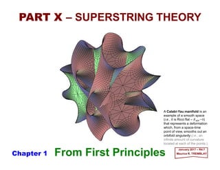
  • 1. From First Principles January 2017 – R4.7 Maurice R. TREMBLAY PART X – SUPERSTRING THEORY A Calabi-Yau manifold is an example of a smooth space (i.e., it is Ricci flat – RΜΝ =0) that represents a deformation which, from a space-time point of view, smooths out an orbifold singularity (i.e., an infinite amount of curvature located at each of the points.) Chapter 1
  • 2. In 1964, Feynman said in his Lectures on Quantum Mechanics (Vol. III): “I think I can safely say that nobody understands quantum mechanics.” Well, that was back in the day when he worked on a quantum theory of gravitation (c.f., Acta Phys. Pol.) and if he were to extend the point particle idea to that of a vibrating string and develop a theory that des- cribes energy and matter as being composed of tiny, wiggling strands of energy that look like strings, then surely he would say: “I think I can safely say that only Ed Witten under- stands string theory.” So, in no way does this set of slides come close to the height of his intellect but it is meant to provide at least some familiarity to study the more established and serious textbooks on the subject (c.f., References) and spearhead some gifted kid!* Forward 2 2017 MRT As with my other work, nothing of this is new or even developed first hand and frankly it is a rearranged compilation of various quotes from various sources (c.f., ibid) that aims to display an abridged but yet concise and straightforward mathematicaldevelopment of string theory and superstrings (and some compactificationas a consequence) as I have understood it and wish it to be presented to the layman or to the inquisitive person. Now, as a matter of convention,I have included the setting h≡c≡1 in most of the equations and ancillary theoretical discussions and I use the summation convention that implies the summation over any repeated indices (typically subscript-superscript) in an equation. * In order for someone to do active string theory research today, you have to be a very smart and committed person…Seriously! Anyhow, this is my take on string theory… It will be work in progress (in three parts probably) for some time to come as I myself mature and develop skills to make sense of it all. String theory is a tough subject and it does require mathematical and physical intu- ition that is so daunting but it will be quite a challenging experience to unravel some of it!
  • 3. Contents of 2-chapter PART X 2017 MRT PART X – SUPERSTRING THEORY A History of the Origins of String Theories The Classical Bosonic String The Quantum Bosonic String The Interacting String Fermions in String Theories String Quantum Numbers Anomalies The Heterotic String Compactification and N=1 SUSY Compactification and Chiral Fermions Compactification and Symmetry Breaking Epilogue: Quantum Gravity Appendix I: The Gamma Function Appendix II: The Beta Function Appendix III: Feynman’s Take on Gravitation Appendix IV: Review of Supersymmetry “We propose that the ten-dimensional E8×E8 heterotic string is related to an eleven-dimensional theory on the orbifold R10×S1/Z2 in the same way that the Type IIA string in ten dimensions is related to R10×S1. This in particular determines the strong coupling behavior of the ten-dimensional E8×E8 theory. […]” Petr Hořava and Edward Witten, Preface to their paper prescribing M-Theory for the first time (1995). Appendix V: A Brief Review of Groups and Forms References
  • 4. Contents 2017 MRT PART X – SUPERSTRING THEORY A History of the Origins of String Theories The Classical Bosonic String The Quantum Bosonic String The Interacting String Fermions in String Theories String Quantum Numbers Anomalies The Heterotic String Compactification and N=1 SUSY Compactification and Chiral Fermions Compactification and Symmetry Breaking Epilogue: Quantum Gravity Appendix I: The Gamma Function Appendix II: The Beta Function Appendix III: Feynman’s Take on Gravitation Appendix IV: Review of Supersymmetry Appendix V: A Brief Review of Groups and Forms References
  • 5. The story of the development of string theories is such a beautiful example of the disorganized and unpredictable way in which elementary particle theory has evolved that we cannot resist the temptation to give a brief historical (i.e., mathematical) introduction. 5 2017 MRT A History of the Origins of String Theories During the early 1960s, particle physics, or at least the strong-interaction sector which was receiving the most attention, both theoretical and experimental, was dominated by S-matrix theory. Its basic ingredients were the general properties of the scattering matrix or S-matrix (N.B., the S-matrix elements are given by 〈 f |S|i〉 which are the probability amplitudes for the transition between an initial state i and a final state f ) rather than fundamental fields described by Lagrangians. The S-matrix was expected to be determined mainly by the requirements of analyticity, crossing, and unitarity, terms which we shall now explain. In their seminal two-volume treatise (suitable for an ‘advanced’ graduate-level course), M. Green,J. Schwarz and E. Witten, Superstring Theory, Vol. I - Introduction, Cambridge University Press (1987), Section 1.1 entitledThe Early Days of Dual Models, gives a more detailed and systematic study than the rough outline that is presented in this chapter. That first section of their book begins with the paragraph: “In 1900, in the course of trying to fit to experimental data, Planck wrote down his celebrated formula for blackbody radiation (i.e., I(ν,T )=(2hν 3/c2){1/[exp(hν/kBT )−1]}). It does not usually happen in physics that an experimental curve is directly related by a more or less intricate chain of calculations. But blackbody radiation was a lucky exception to this rule. In fitting to experimental curves, Planck wrote down a formula that directly led […] to the concept of the quantum.”
  • 6. It is convenient to write the S-matrix as the sum: 6 2017 MRT 22 )()( dcba pppps +=+≡ AiS += 1 where 1 is the unit matrix representing processes in which the particles do not interact, and A is the scattering amplitude. The analyticity assumption is that A must be an analytic function of the Lorentz invariants that describe the process, with only isolated singularities that are determined by the spinless particles (c.f., PART VIII – THE STANDARD MODEL: Scattering Experiments): dcba +→+ This is an analytic function of the two-independent Lorentz invariants that can be formed from the four-momenta (i.e., pa ≡pa µ, &c.) of the particles: and: 22 )()( dbca ppppt −=−≡ referred to as s-channel and t-channel, respectively. The Diagram below shows the flow. There is also u=(pa −pd)2 =(pb −pc)2. s, t, and u are the well-known Mandelstam variables. ++ ↑↑↑↑ +→+ dcba −− ↑↑↑↑ +→+ dcba s-channel t-channel
  • 7. The amplitude will contain poles corresponding to the propagators of single particles. For example, a particle of spin J and mass M coupling to the state a+b will give a pole of the form: 7 2017 MRT L+ − = 221 )( ),( Ms zP ggtsA sJ where g1 and g2 are the coupling constants (see Figure), PJ a Legendre function and zs is the cosine of the scattering angle in the center-of-mass system. In the simple case when the masses of the external particles are all equal to m, we readily calculate from the t- channel process t=4m2 −2E2 +2|p|2 cosθ (c.f., op cit) that zs =1+2t/(s−4m2). The physical region of the variables for this so-called s-channel process is given by the conditions: 04 2 ≤≥ tms and Processes giving (Left) an s-channel pole at s=M2 and (Right) a t-channel pole at t =M2. s t Mg1 g2 a b c d s t M g′1 g′2 a b c d
  • 8. Crossing is the assumption that the same scattering amplitude, analytically continued to appropriate regions of the variables, also describes the crossed processes: 8 2017 MRT 04 2 ≤≥ smt and The physical region for the first of these (called the t-channel process because in this case t≡(pa −pc)2 =(pb −pd)2 gives the total center-of-mass energy) is: bcdadbca +→++→+ and Crossing requires that the amplitude has poles, analogous to those of A(s,t) above: L+ − ′′= 221 )( ),( Mt zP ggtsA tJ The other main ingredient of S-matrix theory is that S is unitary: 1=SS† in any physical region for any given process. This ensures the conservation of probability (i.e., that the sum over all the possible things that can happen is unity or always 100% every time, if you wish). We note that the sum over all possible intermediate states implied in the matrix multiplication S†S=1 above automatically couples together an infinite sequence of possible processes. Also, since only those states that are energetically possible can contribute, unitarity requires the existence of new singularities at each new threshold. They are branch points, the first of which occurs at s=4m2 in our example above. More generally, they arise at values of s equal to the square of the sum of the masses of the particles in the intermediate state.
  • 9. In order to make calculations in S-matrix theory, use was made of various pole approximations. Clearly, in the neighborhood of a pole (e.g., s≈M2), that pole will dominate the amplitude. Because of the large number of resonances, it seemed reasonable to guess that a sum over such resonances: 9 2017 MRT ∑ − = i i sJ ii Ms zP ggtsA i 221 )( ),( might be a fair approximation to the amplitude in the physical s-channel region. Note that the above lowest s-channel threshold the states are unstable, so the masses are complex, Mi →Mi −½iΓi , the imaginary part being the decay width Γi. The t-channel poles, on the other hand, give the forces that dominate forward scattering (i.e., zs ≅1 so t is near zero). However, a t-channel pole corresponding to a particle of high spin would give an unacceptable contribution at high s, since it behaves like: JJ ttJ tJ szzPtsA Mt zP ggtsA ~~)(~),( )( ),( 221 →+ − ′′= L at fixed t whereas unitarity can be shown to allow only amplitudes growing no faster than s.
  • 10. Now, in order to understand the significance of such t-channel poles for the s-channel scattering process, it is necessary to make a partial-wave expansion in the t-channel and to define an analytic continuation of the partial-wave amplitude to complex values of the angular momentum J. The poles then occur along so called Regge trajectories: 10 The solutions of this equation for integer values of J give the mass-squared of the particle, the value of J being its spin. A typical Regge trajectory. This trajectory connects a particle of mass m1 2 and spin- 1 and a particle of mass m2 2 and spin-2. There is also a spin-0 tachyon state ( ) of negative [mass]2, which must be removed by having zero residue. 2017 MRT For example, a nonrelativistic three dimensional harmonic oscillator of classical frequency ω has the energy eigenvalues:       ++ω=      +ω= 2 3 2 2 3 , JnnE rJn hh where nr is the radial quantum number and J is the orbital angular momentum. Although J is quantized (J=1,2,…) this equation can be regarded as giving the mass of the bound states Mn,J (=En,J) as a function of J. We can invert it to write the Regge trajectory: )( 2 3 2 2 Mn M J r α≡−− ω = h More generally, a Regge trajectory connects particles with the same internal quantum numbers but different spins (see Figure). )(sJ α= s α(s) m1 2 m2 2 1 2 )(sJ α= −m0 2 0
  • 11. The t-channel partial wave expansion does not converge in the s-channel physical region, but it is possible to replace the sum over integer J by a contour integral in the complex J plane which is well defined everywhere. For high s, this integral is dominated by the rightmost singularities in the J plane, which under suitable assumptions, will be Regge poles. We therefore obtain an approximation of the form: 11 2017 MRT ∑i t i i sttsA )( )(~),( α β showing that the large s amplitude at fixed t is dominated by the leading Regge trajectories (i.e., those with the largest αi(t)). Thus, the high-energy behavior of a given s-channel process is determined by the particles that can be exchanged in the t-channel (i.e., those with the t-channel quantum numbers). The equations A(s,t)=Σigi1gi2[Pzi (zs)/(s−Mi 2)] and A(s,t)~Σi βi(t)sαi(t) above are approximate expressions for the scattering amplitude in terms of the s- and t-channel poles, respectively. They have very different analytic forms but, if both are reasonable approximations to the amplitude in part of the physical region, they must be approximately equal to each other, at least in some average sense. This is the assumption of duality (i.e., the resonances approximately equal Regge poles) for hadron scattering: ∑∑ ≅ − i t i i i sJ ii ii st Ms zP gg )( 221 )( )( α β
  • 12. In 1968, Veneziano proposed the following toy model of a scattering amplitude A that satisfies duality: 12 Regge trajectories of the Veneziano model (with scattering amplitude: A(s,t)= Γ[−α(s)]Γ[−α(t)]/Γ[−α(s)−α(t)]. 2017 MRT It has s- and t-channel poles corresponding to particles of all spins J=0,1,2,…, whose masses are given by the solutions of: JM =)( 2 α (see Figure), because Γ(x) has poles at x= 0,−1,−2,…. Also, since: ba x x bx ax − ∞→  → +Γ +Γ )( )( the Veneziano amplitude also has the Regge asymptotic behavior of A(s,t)~Σi βi(t)sαi(t) as s→∞ at fixed t. It can be shown that it fully satisfies the duality hypothesis in the sense that the sum over the infinite set of s-channel poles reproduces this Regge behavior. ∫ −−−− −=−−= −−Γ −Γ−Γ = 1 0 1)(1)( )1()](),([ )]()([ )]([)]([ ),( ts xxxdtsB ts ts tsA αα αα αα αα where s and t are the Mandelstam variables from above, B is the combination of Euler Gamma functions, Γ, known as the Beta function. This expression is clearly crossing symmetric under s↔t and, provided the Regge trajectory function α(s) is linear: ss ααα ′+= )0()( where α′ is the slope and α(0) the intercept of the trajectory. s α(s) 1 2 3 sd sd )(α α =′ )0(α
  • 13. Generalization to more complicated amplitudes, such as many-particle production processes, we soon made and, for a time, there was much activity trying to fit such dual- model Veneziano amplitudes to experimental data. Even a year later, in 1969, Virasoro generalized Veneziano amplitude by using the four-point function: 13 2017 MRT The next step was to try to deduce these dual-model amplitudes from some underlying dynamics, and the key here was the realization that the spectrum of states is that of a relativistic string. It was then found that the interaction of two open strings led automatically to the existence of closed strings. The dual-string model required a new trajectory to have a slope α ′/2, in rough agreement with experiment. However, a major problem is that the particle poles are all on the real axis, whereas in reality they should lie below this axis if they are to correspond to unstable particles (i.e., if their masses are above the physical threshold). Attempts to correct this by putting branch points into the function α(s) are not successful because they destroy the linearity that is essential to achieve the other satisfactory properties of the model. Thus, dual models came to be seen as just the first-order term in some type of expansion, in which the higher-order terms would ensure unitarity and push the poles off the real axis. )](½)(½[)](½)(½[)](½)(½[ )](½[)](½[)](½[ ),( utusts uts tsA αααααα ααα −−Γ−−Γ−−Γ −Γ−Γ−Γ =
  • 14. In spite of interesting work on a possible dynamical theory underlying dual models, and some success with its phenomenology, interest in the dual model of hadron declined during the early 1970s. Serious obstacles were that self-consistency required that the ground state of the closed string must have spin-2, rather than the spin-1 required for the Pomeron (i.e., a particle that was invented to explain the behavior of elastic-scattering cross sections), and that the models are only fully satisfactory in higher-dimensional spaces. Also, the clear evidence for a parton-like behavior in deep inelastic scattering suggested the existence of pointlike constituents within hadrons and led to the reinstatement of field theory, with quarks and gluons as the new fundamental fields. The idea that hadrons are a self-consistent set of states uniquely determined just by the postulates of S-matrix theory (i.e., the bootstrap hypothesis) became untenable. 14 2017 MRT The dual model, however, lived on. It survived by abandoning hadron physics and becoming instead a candidate theory of the fundamental particles. All of this stemmed from a suggestion by Scherk and Schwarz (1974) that the spin-2 value for the closed string ground state should be taken as an indication that the theory contains gravity, and that the slope α ′ should be taken as O(EP −2) (EP being the Planck energy), so that only the ground states of the strings with mass<<MP ≡EP /c2 are observed in normal physics. Instead their role is to improve the chance of obtaining a finite theory of all interactions, including gravity, by modifying the very short-distance behavior. However, higher dimen- sionality is required and it is hoped that a suitable compactification scheme, ideally one forced by the theory rather than selected by us to produce the required results, will lead to something like the standard supersymmetry (SUSY) model for E<<EP.
  • 15. The ultraviolet (i.e., large-momentum or short-distance) infinities of field theory (i.e., the realm of Renormalization Theory) have their origin in the supposed pointlike nature of elementary particles, and are indeed related to the well-known divergence of the electromagnetic self-energy of a classical point charge. It is, therefore, natural to wonder whether the idea that elementary particles as points should be instead considered as extended objects. (N.B., We are not thinking of extension in the sense that the proton, for example, has finite size owing to the spatial distribution of its pointlike constituents – the quarks. Rather, we are introducing size as an intrinsic property of even elementary objects). 15 The Classical Bosonic String A particle trajectory xµ =xµ(τ) between τ1 and τ2. 2017 MRT We recall from Sp=−m ∫dτ √(gµν xµxν ) of the PART IX – SUPER- SYMMETRY: The Newtonian Limit chapter that the action for such a particle is proportional to path length (see Figure): ∫ ⋅−= xxdmSp &&τ where x ≡dx/dτ (N.B., x is shorthand for xµ) and τ is the para- meter used to label positions on the trajectory. Minimization of this action with respect to variations in xµ(τ) yields ∂[xµ/√(x⋅x)]/∂τ =0. If we choose τ as the proper time, this gives the expected result (c.f., xρ+Γρ µν xµ xν =0 with no gravitational fields – i.e., gµν =ηµν so Γρ µν =0). The momentum conjugate to xµ is given by: ⋅⋅⋅⋅ ⋅⋅⋅⋅ ⋅⋅⋅⋅ from which we obtain (N.B., p is also shorthand for pµ): ⋅⋅⋅⋅ ⋅⋅⋅⋅ ⋅⋅⋅⋅ ⋅⋅⋅⋅⋅⋅⋅⋅⋅⋅⋅⋅⋅⋅⋅⋅ xx xm x L p && & & ⋅ == µ µ µ δ δ 2 mpp =⋅ x2 x0 τ1 τ2 x1
  • 16. We now generalize these results to a one-dimensional extended object (i.e., a string). We require the string to have a finite length, so it can be either an open string, with two free ends, or a closed string, with no free ends but loops around itself. The trajectories followed by such strings are two dimensional surfaces in space-time (see Figure). 16 Parameters τ and σ label the time and space directions, respectively, so that σ1 labels a particular point on the string. (Left) A typical trajectory for an open string. (Right) A typical trajectory for a closed string. 2017 MRT These surfaces can be labeled by two parameters τ and σ such that the space-time coordinate is: x2 x1 x0 τ1 τ2 σ1 x2 x1 x0 τ1 τ2 σ1 xµ(τ,σ)xµ(τ,σ) where µ =0,1,…,(D −1) with D being the dimension (e.g., D=4 is 4D). We will normally think of τ as labeling the time and σ the space direction. For the open string, we choose 0≤σ ≤π and, correspondingly, for the closed string we impose that xµ(τ,σ +π)=xµ(τ,σ). ),( στµµ xx = 0 ≤σ ≤π xµ(τ,σ +π)=xµ(τ,σ)
  • 17. The obvious generalization of the path length Sp =−m∫dτ √(x⋅x) above is to take the action of a string to be proportional to the area of the surface mapped out as it moves between τ1 and τ2. Thus, we put, where we reinsert the constants h and c for clarity: 17 2017 MRT where x′≡∂x/∂σ and where α ′ is a parameter that will later turn out to be the slope of the Regge trajectory associated with the string. Alternatively, (2πα ′hc)−1 represents the tension To in the string. Up to factors of h and c, the string length is the square root of α ′: ∫=′⋅′⋅−′⋅ ′π −= 2 1 1 ))(()( 2 1 2 τ τ τσ α ddL c Sxxxxxx c L and&&& h ⋅⋅⋅⋅ ⋅⋅⋅⋅ The classical equation of motion for the closed string, obtained by minimizing S, is (c.f., the Euler-Lagrange equation of PART VIII – THE STANDARD MODEL: Field Equations): 0=        ′∂ ∂ +        ∂ ∂ µµ δ δ σδ δ τ x L x L & or, explicitly: 0 )()()()( =         ′⋅−′⋅ ∂ ∂ +         ′⋅′−′′⋅ ∂ ∂ L xxxxxx L xxxxxx µµµµ στ &&&&&& This is a very complicated equation of motion! (N.B., L→√[(x⋅x′)2 −(x⋅x)(x′⋅x′)]!) oπ2 1 T cs α α ′ =′= hl ⋅⋅⋅⋅ ⋅⋅⋅⋅ ⋅⋅⋅⋅
  • 18. This last equation above can be simplified if we use the freedom of reparametrization invariance to require that the σ and τ directions be orthogonal (see Figure): 18 2017 MRT 0=′⋅ xx& and also scale σ,τ so that the distance moved when σ changes by dσ is equal to that moved when τ changes by dτ =dσ. Recalling that these distances are spacelike and timelike, respectively, we can write this condition as: 0=′⋅′+⋅ xxxx && Illustrating orthonormal coordinates on the open string trajectory. For some purposes it is useful to remove the remaining freedom in τ and σ by putting: )()constant( µ µτ xn= where n is a constant vector. One particular choice of n, in which it has the components: so it is on the light-cone: ]1...,,0,0,1[ 2 1 −=µn When these two last conditions above are satisfied, we are said to be using an orthonormal or conformal gauge. In such a gauge, the equation of motion above becomes the familiar wave equation: µµ xx ′′=&& leads to the so-called light-cone or transverse gauge. 0=⋅nn τ1 σ1 σ2 σ3 τ2 τ3
  • 19. With xµ =x″µ above, we can write the general solution for a closed string in the form: 19 2017 MRT and: where XL µ, XR µ are arbitrary, twice-differentiable, functions that represent waves traveling in opposite directions ( left and right , respectively) around the closed string. The boundary condition xµ(τ,σ +π)=xµ(τ,σ) above implies that they can be written in the form: )()(),( στστστ µµµ −++= RL XXx ⋅⋅⋅⋅⋅⋅⋅⋅ ∑≠ +− +++= ′ 0 )(2 0 e 1 2 )( 2 1 2 1 n niL nL n i qX στµµµµ αστα α ∑≠ −− +−+= ′ 0 )(2 0 e 1 2 )( 2 1 2 1 n niR nR n i qX στµµµµ αστα α where qµ, α0 µ, and (α µ)n L,R are all Lorentz vectors, with qµ and α0 µ being real (N.B., these are the center-of-mass position and momentum of the string, respectively) and with: *)( ,, RL n RL n −= αα (N.B., The Fourier decompositions XL µ/√(2α′) and XR µ/√(2α′) above will be essential to quantize the string. Then the αs will have an interpretation as creation/annihilation operators and the inclusion of the factors √(2α ′) and 1/n will give an appropriate normalization to the αn parameters.)
  • 20. The apparent simplicity of the solution xµ(τ,σ)= XL µ(τ +σ)+XR µ(τ −σ) is spoilt by the above constraints (i.e., x⋅x′=0 and x⋅x+ x′⋅x′=0) which become: 20 2017 MRT must be zero, that is: Using XL,R µ/√(2α′) above, these equations imply that the so-called Virasoro generators defined by: 0=⋅=⋅ RRLL XXXX &&&& ⋅⋅⋅⋅ ⋅⋅⋅⋅ ⋅⋅⋅⋅ ∑ +∞ −∞= −⋅−≡ k L kn L k L nL αα 2 1 The closed string that we have considered here is oriented in the sense that changing σ →−σ generally changes the solution. It is possible to consider an unoriented closed string on which we impose invariance under σ →−σ. Clearly, from xµ(τ,σ)= XL µ(τ +σ)+ XR µ(τ −σ) above, this requires: ( )stringclosedunorientedµµ RL XX = ( )nLL R n L n 0 allfor== ∑ +∞ −∞= −⋅−≡ k R kn R k R nL αα 2 1 and
  • 21. The open string can be treated in a similar way, but a new problem arises: minimiza- tion of the action does not lead to the Euler-Lagrange equation of motion above because of the contributions of boundary terms at σ =0 and π. These stem from the integration by parts. In order to remove the boundary terms, we require that open strings satisfy the boundary conditions: 21 2017 MRT Given x′µ(τ,0)=x′µ(τ,π)=0 above we can proceed as before, except that for open strings we need the standing-wave solution: Equation x⋅x+ x′⋅x′=0 above then implies that x⋅x=0 at σ =0 and σ =π (i.e., that the ends of the string move with the velocity of light!) 0),()0,( =π′=′ ττ µµ xx ⋅⋅⋅⋅ ⋅⋅⋅⋅ ⋅ ⋅ )cos(e 1 ),( 2 1 0 0 σαταστ α τµµµµ ∑≠ − ++= ′ n ni n n n iqx where again qµ and α0 µ are real and: *)( µµ αα nn −= As before, the constraint equations (i.e., x⋅x′=0 and x⋅x+ x′⋅x′=0) imply that:⋅⋅⋅⋅ ⋅⋅⋅⋅ ⋅⋅⋅⋅ 0 2 1 =⋅−≡ ∑ +∞ −∞= − k knknL αα
  • 22. It is possible to simplify the constrain equations if we work in the light-cone gauge, defined by τ =(constant)(nµ xµ) and nµ=(1/√2)[1,0,0,…,−1] above. For this purpose we introduce D-dimensional light-cone coordinates: 22 2017 MRT where bold-face quantities are vectors in the (D−2)-dimensional transverse space, with components x1, x2, …, xD−2. Also, from τ =(constant)(nµ xµ) and nµ=(1/√2)[1,0,0,…,−1] above: which, to put things into perspective, reduces to the x± ≡(1/√2)(x0 ±x3) and x1, x2 light- cone coordinates (x1, x2 being transverse coordinates) when D=4 is taken to be physical space-time. Then any vectors x and y satisfy:      ±≡ − −± 221 10 ,,, )( 2 1 D D xxx xxx K yx ⋅⋅⋅⋅−=⋅ −+ xxyx + = x)constant(τ and hence in xµ(τ,σ)/√(2α ′) above, q+ and αn + (n≠0) are zero. Thus, the constraint Ln ≡ −½Σkαk ⋅αn−k =0 above becomes an equation for αn −: ∑ +∞ −∞= −+ − = k knkn αααα⋅⋅⋅⋅αααα 0 1 α α showing that the only degrees of freedom are α0 +, q−, and the transverse modes ααααk.
  • 23. Similarly, for the closed string, τ =(constant)x+ above (N.B., recall that we also defined x± ≡(1/√2)(x0 ±x3) above) implies that (α n +)L,R =0 (for all n≠0), so the constraints give: 23 2017 MRT in the conformal gauge. The total momentum of the string is obtained by integrating pµ over the whole string: We calculate the momentum as for a point particle: ∑ −+ − = k L kn L k L n αααα⋅⋅⋅⋅αααα 0 1 )( α α αδ δ µ µ µ ′π == 2 x x L p & & µµµµ α α αα α σ 00 2/1 0 2 2)2( 2 1 ′ =π′ ′π == ∫ π pdP for the closed string, and: µµµ α α α α 00 2 12 2 1 ′ = ′ =P for the open string. showing that the only degrees of freedom are α0 +, q−, and the transverse modes (ααααk)L,R. ∑ −+ − = k R kn R k R n αααα⋅⋅⋅⋅αααα 0 1 )( α α and ( )movers ( )movers Left Right
  • 24. These equations determine the mass of the string. For the closed string we have: 24 2017 MRT In the light-cone gauge, these last two equations for the M2 of closed and open strings become: where to obtain the last line we have used the zero-frequency constraints Ln L=Ln R =0 (for all n) above (N.B., Ln L=Ln R =0 also implies that the L and R contributions to the mass are identical). For the open string we find, similarly: ∑ ∞ = −− ⋅+⋅ ′ −=⋅ ′ =⋅= 1 00 2 )( 22 n R n R n L n L nPPM αααα α αα α ∑ ∞ = − ⋅ ′ −=⋅ ′ = 1 00 2 1 2 1 n nnM αα α αα α and: ( )closed∑ ∞ = −− + ′ = 1 2 )( 2 n R n R n L n L nM αααα⋅⋅⋅⋅αααααααα⋅⋅⋅⋅αααα α ( )open∑ ∞ = − ′ = 1 2 1 n nnM αααα⋅⋅⋅⋅αααα α respectively.
  • 25. Before we proceed to quantize the string, it is of interest to introduce an equivalent classical model defined by the action (c.f., S= ∫τ Ldσ dτ above): 25 2017 MRT where R(D=2)(hab)≡habRab (D=2) is the scalar curvature obtained from hab and where Rab (D=2)= ∂b Γc ac −∂c Γc ab −Γc ab Γd cd +Γc ad Γd bc with Γc ab=½hcd (∂a hbd +∂b had − ∂d hab ). However, in two dimensions, such a term is a constant that does not affect the dynamics! where h=−det(hab) with hab the metric on the two-dimensional world-sheet of the string. The indices a,b take values 0,1 (N.B., ξ 0, ξ 1 here play the roles of τ,σ used earlier). We can think of the action S above as describing a set of D=2 scalar fields xµ(ξ 0,ξ 1) on a two-dimensional space-time, with background metric hab (i.e., the usual space-time variables have become scalar fields). Such an interpretation suggests several possible generalizations. One fairly obvious possibility is to add to S above the action of Einstein’s gravity on the two-dimensional world-sheet: ba ab xx hhddS ξξ ξξ α ∂ ∂ ⋅ ∂ ∂ ′π −= ∫ 10 4 1 )()2(10)2( abDD hRhddS == ∫= ξξ The equivalence of S= ∫τ Ldσ dτ and S above, as classical theories, can be demons- trated by finding the Euler-Lagrange equation corresponding to variations in hab, solving it, and using the solution to eliminate hab from S above, thereby recovering the action S= ∫τ Ldσ dτ. However, such an equivalence does not in general hold in quantum theory because of the quantum fluctuations about the minimum solution for hab.
  • 26. More can be said about the nature of these fluctuations by noting that hab, being sym- metric, is defined by three independent functions of ξ 0,ξ 1. The freedom to reparametrize (i.e., reparametrization invariance) allows us to introduce two new arbitrary functions: 26 2017 MRT and so the only remaining degree of freedom is the scale (or conformal) factor φ(ξ 0,ξ 1). When we insert this hab into S above the factor φ clearly cancels and so plays no role in the classical equations. In fact, with hab above, we can write S as:* for a=1,2, which can be chosen so that hab has the form: ),( 10 ξξξξ aa ′=′ baba h ηξξφξξφ ),( 10 01 ),( 1010 =      − = ba ab xx ddS ξξ ηξξ α ∂ ∂ ⋅ ∂ ∂ ′π −= ∫ 10 4 1 * Green, Schwarz & Witten (c.f., § 1.3.3), in their notation, use, hαβ =ηαβ expφ where expφ is an unknown conformal gauge. Their free field action reduces to S=−(T/2)∫dσ 2ηµνηαβ ∂α Xµ ∂β Xν (with dσ 2 ≡dτ dσ and Xµ=Xµ(τ,σ) is their label for string position).
  • 27. In quantum theory it is necessary to do a path integral over all metrics and all trajectories x(ξ a). This requires us to define suitable weights for the path integrals and to remove the divergences that arise. A. M. Polyakov (1981) showed that S above is equivalent to S= ∫τ Ldσ dτ if, and only if, the dimension of space-time is D=26! This cancellation of divergences, which seems to be essential for a consistent string theory, is referred to as the cancellation of the conformal anomaly where Lorentz invariance is only established in the critical dimension for bosonic strings: In the above discussion we have implicitly assumed that the background (i.e., D=26) space-time is flat (i.e., gµν =ηµν ) – we have ignored gravity! Since the string automati- cally contains gravity, this is inconsistent. The correct requirement for conformal invariance to hold is that the background metric should satisfy an equation that, in lowest order, reduces to Einstein’s equation Rµν −½Rgµν=−κ 2Tµν (c.f., PART IX – SUPERSYM- METRY: The Inclusion of Matter or Appendix III: Feynman’s Take on Gravitation for a field theory derivation of gravitation). 27 2017 MRT 26=D
  • 28. The quantization of a classical system is not always a uniquely defined procedure. The classical limit can be regarded as the first term of an expansion in powers of h and there is clearly an infinite number of possible expansions that have the same zeroth-order limit. Several methods of quantizing the classical string, based on the analogy with point- particle models, have been used, and the results agree provided that certain consistency conditions are satisfied. 28 2017 MRT Here we use the canonical quantization method (as opposed to light-cone gauge quantization) in which we regard xµ(τ,σ) and its conjugate momentum pµ(τ,σ)=xµ/2πα′ as operators that satisfy the equal-time commutation relation: The Quantum Bosonic String ⋅⋅⋅⋅ )()],(),,([ σσδστστ νµνµ ′−−=′ gipx Using the Fourier expansion xµ(τ,σ)/√(2α′)=qµ +α0 µ +iΣn≠0(1/n)αn µ exp(−inτ)cos(nσ) for the open string, we see that this relation requires: νµνµ α giq −=],[ 0 all the other commutators being zero. Using αm µ =(α−m µ)† we can replace [αm µ †,αn ν] above by: νµνµ δαα gn nmnm =],[ † which shows that we can regard αn and its adjoint αn †, for positive n, as annihilation and creation operators, respectively. and: νµνµ δαα gm mnnm 0,],[ +−=
  • 29. We shall now impose the constraint Ln ≡−½Σk=±∞ αk ⋅αn−k =0 of the The Classical Bosonic String chapter by working in the light-cone gauge (N.B., there is also the Lorentz covariant quantization approach which will not be used here). Since there is no longitudinal motion, this means that only the transverse operators αn ν used in the canonical quantization method (where ν =1,2,…,D−2) represent independent degrees of freedom, and for these: 29 2017 MRT assuming the background is flat (i.e., gµν =ηµν). It should be noted, however, that this choice of gauge breaks the explicit Lorentz invariance of the theory, which is the source of a difficulty that we shall encounter below. ˆ ˆ νµνµ δδαα ˆˆˆ†ˆ ],[ nmnm n−= The vacuum state, |0〉, can be defined as the eigenstate of all the annihilation operators, αn µ (n positive), that has zero eigenvalues:ˆ ( )...,2,1,000ˆ == nn µ α Other states of the system can be obtained by acting on |0〉 with the creation operators α−1 ν, α−2 ν, &c.ˆ ˆ
  • 30. We can calculate the mass of the resulting states by using the mass operators given by M2 =(1/2α′)α0 ⋅α0 of the The Classical Bosonic String chapter. However, when we relate this to the αn operators by means of the constraints (i.e., to obtain the analog of M2 =−(1/α′)Σnα−n⋅αn), we meet a new problem. The operators must be normal ordered (i.e., all the annihilation operators must be placed to the right of all the creation operators). Since the order is irrelevant for classical quantities, and each change of order introduces a constant as in [αm µ†,αn ν ]=−nδmnδ µν above, the reordering required to produce the quantized expression introduces an arbitrary constant. Thus, instead of M2 = −(1/α′)Σnα−n⋅αn of the The Classical Bosonic String chapter we write: 30 2017 MRT where the number operator N is defined to be: )]0([ 12 α α − ′ = NM ∑ ∞ = −= 1n nnN αααα⋅⋅⋅⋅αααα in the light-cone gauge, and where we have called the unknown constant α(0). The reason for this choice is that, if we rewrite M2 =(1/α′)[N−α(0)] above in the form: 2 )0( MN αα ′+= it becomes reminiscent of the linear Regge trajectory of slope α ′ and intercept α(0) as in α(s)=α(0)+α ′s of the A History of the Origins of String Theories chapter, if N is interpreted as the angular momentum. ˆˆ ˆˆ
  • 31. In order to study the angular momenta of the states, we need the angular-momentum operators: 31 2017 MRT which are generalizations of the angular momentum in three dimensions discussed in PART IX – SUPERSYMMETRY: The SUSY Algebra chapter or Appendix IV: Review of Supersymmetry. In the The Classical Bosonic String chapter,we used the expansion [1/√(2α′)]xµ(τ,σ)=qµ +αm µτ +iΣn≠0(1/n)αn µ ⋅exp(−inτ)cos(nσ) and this becomes: ∫ −= π 0 )( µννµµν σ pxpxdM ∑ ∞ = −− − +−= 1 00 )( )( n nnnn n iqqM µννµ µννµµν αααα αα We can use this expression to calculate explicitly the commutation relations of the different components of Mµν. These do not turn out to be exactly what one would expect for angular momentum. In particular, when we use (±) light-cone gauge coordinates x± ≡ (1/√2)(x0 ± xD−1), and calculate the commutation relations between the components M−µ (where µ are the transverse coordinates as in [αm µ†,αn ν ]=−nδmnδ µν above), we obtain:ˆˆ ˆˆ ˆ ˆ ∑ ∞ = −−+ −− −∆ ′ −= 1 ˆˆˆˆ 2 0 ˆˆ ][ )( 2 ],[ m mmmmmMM µννµνµ αααα α α instead of zero, which would be expected if Mµν obeyed the usual angular-momentum commutation relations: nspermutatiocyclic],[ += σνρµσρµν η MMM
  • 32. The quantity ∆m in [M−µ,M−ν] above turns out to be: 32 2017 MRT So it appears that by working in a particular Lorentz frame (i.e., using the light-cone gauge) we have lost Lorentz invariance and that our string theory is inconsistent (i.e., since ∆m ≠0). However, this problem does not arise if we impose the conditions: m D m D m 1 )]0(1[2 12 26 12 26       −+ − +      − ≡∆ α ˆˆ 1)0(26 == αandD because then ∆m ≡0 and the required commutation relations hold. The existence of these consistency conditions is a remarkable new feature of strings as compared to point particles. The masses of the states, and the dimension of space- time in which they can exist, are uniquely specified. The ground state, with N=0, is, according to N=α(0)+α ′M2, a tachyon (i.e., it has negative [mass]2): α′ −= 12 M where we are always taking α ′, which gives the string tension, to be positive. The first excited state is: 01 ˆ 1 µ α−= is massless and has spin-1. It has the expected 24 transverse degrees of freedom associated with a massless vector particle in D=26 dimensions.
  • 33. This last remark offers a quick way of understanding the reason for the constraint α(0) =1 above. If the states in |1〉=α−1 µ |0〉 had a finite mass there would be an inconsistency because their longitudinal degrees of freedom would be missing. And given the value of α(0) we can understand why we need D=26. We first write M2 =(1/α′)Σnαααα−n⋅⋅⋅⋅ααααn (for an open string) of the The Classical Bosonic String chapter in the form: 33 2017 MRT ∑ ∞ = −− + ′ = 1 2 )( 2 1 n nnnnM αααα⋅⋅⋅⋅αααααααα⋅⋅⋅⋅αααα α that is, with the two possible orderings included equally. If we regard this equation as the definition of the quantum operator M2, and put the ααααn into normal order, we find: ˆ ∑∑∑∑ ∞ = ∞ = − ∞ = − ′ − + ′ = ′ + ′ = 1ˆ 1 ˆˆ 1 2 2 21 ”“],[ 2 11 ”“ nn nn n nn n D NM αα αα αα µ µµ αααα⋅⋅⋅⋅αααα where in the last equation we have used [αm µ†,αn ν ]=−nδmnδ µν above with αm † =α−m. These supposed equalities (i.e., “=”) have been put in quotes because strictly they are meaningless, since the final sum does not converge. It can, however, be given a meaning by using zeta-function regularization. ˆˆ ˆˆ
  • 34. To this end, we note that the Riemann zeta-function ζ(s) is given by: 34 2017 MRT ( )1Re)( 1 >= ∑ ∞ = − sns n s forζ and can also be represented by: ∫ ∞ − − − −Γ = 0 1 e1 e )( 1 )( t t s ttd s sζ for Res>0. This last integral can be analytically continued to Res<0 by doing the integration by parts. In particular, we find that: 12 1 )1( −=−ζ Hence, M2 “=” (1/α′)N+[(D−2)/2α′]Σnn above becomes: αα ′ − − ′ = 24 212 D NM so to get α(0)=1 we require D=26 (c.f., N=α(0)+α ′M2 above).
  • 35. It is important to know whether these conditions on D and α(0) are essential or are merely a consequence of the choice of the method of quantization. Since they stem from the breaking of Lorentz invariance in [αm µ†,αn ν ]=−nδmnδ µν above, it is necessary to see what happens if we quantize in a manifestly Lorentz-invariant manner. However, problems then arise through the occurrence of states of negative norm called ghosts. To understand the origin of these ghosts we start with the vacuum state, |0〉, which has positive norm: 35 2017 MRT 100 = Then we consider the one-particle timelike excitation: ˆˆ ˆˆ 01 0 1 0 −≡ α 00000)(011 0 1 0 1 0 1 †0 1 00 −=== −−− αααα for which: from [αm µ,αn ν ]=−mδn+m,0 gµν above. Thus |10 〉 is a ghost state with negative norm.
  • 36. Since negative norm states are meaningless (e.g., they would give problems with unitarity because they imply a negative probability), we must somehow exclude them from the physical spectrum. Now, from Ln ≡−½Σk=±∞αk ⋅αn−k =0 the The Classical Bosonic String chapter, physical states have to be eigenstates of the Virasoro generators Ln with zero eigenvalues. This condition can only be imposed for positive n, and it suffices to remove the ghosts provided that: 36 2017 MRT 1)0(26 == αandD or: 1)0(26 ≤< αandD Thus, the conditions for the removal of ghosts are somewhat less restrictive than just D= 26 and α(0)=1 alone. However, D=26 appears to be necessary when we consider interacting strings in order to remove the conformal anomaly we mentioned earlier. But there is general agreement that the natural dimension for the quantized bosonic string is D=26.
  • 37. We now briefly discuss the closed string, for which essentially the same procedure can be followed. If we start from the light-cone gauge expression M2 =(2/α′)Σn(αααα−n L⋅ααααn L +αααα−n R⋅ ααααn R) (for a closed string) of the The Classical Bosonic String chapter, again find that we require D=26, and the mass spectrum becomes: 37 2017 MRT ∑ ∞ = −≡ 1 ,,, n RL n RL n RL N αααα⋅⋅⋅⋅αααα where NL and NR are number operators for the left- and right-moving sectors: )2( 22 −+ ′ = RL NNM α which, as before, are required to be equal by the constraints. The slope of the Regge trajectory for the closed string is thus α′/2, and the zero mass state now has spin-2 (NL = NR =1). This concludes our discussion of the quantized bosonic string. We have found that it belongs most naturally in D=26 dimensions. The open string then has a zero-mass spin-1 (vector) boson which the closed string has a zero-mass spin-2 boson. So there are already hints that string theories may contain both Yang-Mills and gravity gauge fields! But the occurrence of the tachyons (i.e., ground states with negative [mass]2) is unsatis-factory. In string theories, we need to impose supersymmetry (c.f., Appendix IV: Review of Supersymmetry) to eliminate the tachyons! Finally, we remind the reader that if 1/α′ in M2 =(1/α′)[N−α(0)] above is O(MP 2) then the excited states of the strings are all expec- ted to have mass O(MP) and hence be unobservable in low-energy particle physics.
  • 38. In this introduction to string theory of the classical and quantum string we only discussed free (bosonic) strings. We must now introduce interactions between the strings. A proper treatment of this topic presumably requires a quantum field theory of strings, with operators that create and annihilate strings, analogous to those employed in a field theory of particles. The Interacting String 38 Here we shall proceed by noting that the chief practical consequence of a field theory of particles is the Feynman diagrams, including the rules for their evaluation. The most primitive Feynman diagram has two particles coming together to form a third (see Figure 1), and more complex diagrams can be built up by joining such primitive diagrams together. a b c Figure 1: A Feynman diagram for the process a +b→ c. 2017 MRT
  • 39. By analogy, we expect that the corresponding theory of strings will have a basic diagram in which two strings join to form a new string. Various possibilities, involving both open string and closed strings, are illustrated in Figure 2. 39 All the other scattering processes can then be obtained by combining together these basic diagrams. 2017 MRT Figure 2: The world-sheets corresponding to (Left) two open strings joining to make an open string, (Middle) two closed strings forming a closed string, and (Right) two open strings joining to make a closed string. Relations between the couplings g, κ, and κ′ are discussed in remark (4) in the slides. g κ′ κ
  • 40. For example, just as we can use the particle diagram of Figure 1 twice in order to obtain the single-particle exchange contribution in both the diagrams (like Figure 2 - Left) to obtain the open-string contribution to open-string scattering shown in Figure 3 - Right. 40 2017 MRT Figure 3: Diagrams (Left) and (Middle) show particle scattering due to single particle exchange; (Right) shows the corresponding closed string amplitude which incudes (Left) and (Middle). A B C D A B C D Y X Y X A B C D
  • 41. We should note, however, some very important differences between the string and particles diagrams: 41 2017 MRT 1. In contrast to point-particle field theories there is apparently no freedom in string interactions, because there is no particular point that can be identified with a vertex. Indeed, every part of a string diagram is simply a freely propagating string in some frame of reference, so there is no Lorentz-invariant way of specifying the space-time point at which the two strings join. We see this by reference to Figure 4. Figure 4: Showing how the intersecting point depends on the choice of time axis. If we choose the time axis t to be horizontal, the strings join at P. On the other hand, if we view the system from a different reference frame in which time is measured along t′, then P is just one end of a freely propagating string. 2. Because of remark (1), the potentially ultraviolet-divergent region of integration, which is Feynman diagrams occur when vertices are close together (i.e., at high momentum transfer), are missing from string diagrams. This is of course the reason why we hope that the field theory of an extended object like a string may be finite. t t′ P
  • 42. 3. There are many fewer string diagrams. For example, the string diagram of Figure 3 - Right contains the particle exchange diagram of Figure 3 - Left corresponding to the exchange of all the particles that are described by the string X (e.g., the infinite sum of states A(s,t)=Σi gi1 gi2 PJi (zs)/(s−Mi 2) of the A History of the Origins of String Theories chapter). Further, Figure 3 - Right can be regarded as describing strings a and b joining to form a single string X, which then splits again, or as strings a and c joining to form the string Y, which subsequently splits. Thus, like A(s,t)=Γ[−α(s)]Γ[−α(t)]/Γ[−α(s)−α(t)] of the A History of the Origins of String Theories chapter, the single string diagram contains both of the particle exchange diagrams Left and Middle of Figure 3. So, whereas the Feynman diagrams, Figure 3 - Left and Middle, have to be added, both are included in the single string diagram of Figure 3 - Right. Similarly, in Figure 5, the one-loop string diagram in Left includes both of the Feynman diagrams shown in Middle and Right. 42 2017 MRTFigure 5: Showing how one string loop diagram (Left) contains two different types of Feynman loop diagrams (Middle) and (Right).
  • 43. 4. The fact that the string diagrams can be interpreted in these different ways means that the various coupling constants are related. Thus, initially the theory may appear to allow three coupling constants g, κ, and κ ′, associated with the three string interactions shown in Figure 2. However, if we consider Figure 6 we see that (reading from left to right) it is a closed+open→closed+open diagram, with coupling constant κκ′. Hence, the coupling constants κ and κ ′ must be equal. 43 2017 MRT Figure 6: An open, open, closed, closed scattering diagram that relates κ and κ ′. If we are hoping to identify one of the states of the closed string with the graviton, this equality is of course essential to ensure that open and closed strings all fall at the same rate in a gravitational field.
  • 44. The other relation that we obtain is, however, new. To derive it we consider the contri- bution to the scattering of two open strings (--) by the one-loop diagram of Figure 7. 44 2017 MRT n g ακ ′= 24 If we interpret this as going from left to right the intermediate state is two open strings (--) so it is: Figure 7: A one-loop diagram for the scattering of two open strings. This diagram relates the gauge and gravitational coupling constants, g and κ respectively. [This convention will be applied henceforth.] where the power of α ′ is n=(D/2)−3, chosen to make the dimensions correct. Note that in D dimensionsg has the dimensionality of [length](D/2)−2, whileκ has [length](D/2)−1 and α ′ has [length]2. whereasif weviewit as going from bottom to top it is oneclosedstring (--) and hence: 4 ~ g Thus, we can relate g4 to κ 2 =κ ′2: 2 ~ κ′ or≡ ≡
  • 45. The argument above was originally used by C. Lovelace in the context of hadronic string theories to show that unitarity required the existence of closed strings, and hence of the pomeron (i.e., a Regge trajectory postulated in 1961 to explain the slowly rising cross section of hadronic collisions at high energies), with a coupling given by g4 =κ 2α ′n above (and do recall that n=(D/2)−3). In the present context, it shows instead the necessity for gravity. The relation between the gravitational coupling κ and the gauge coupling g given in g4 =κ 2α ′n above does not immediately imply anything about the four- dimensional couplings because they have different dimensions, and so the two sides of the equation with be scaled by the compactification volume in different ways. 45 2017 MRT α κ ′ = 2 2 g We shall see later (c.f., The Heterotic String chapter) that the most promising theories are based on a single closed string that contains both the gauge vector particles and the graviton. Then g4 =κ 2α ′n above is replaced by: This relation in dimensionally correct for any value of D and so both sides scale in the same way on compactification. Thus, provided α ′ is of the order of κ 2, the theory predicts gauge couplings that are of O(1) as required.
  • 46. The evaluation of a scattering amplitude relies on the freedom in the choice of the world-sheet metric, which was mentioned at the end of the The Classical Bosonic String chapter. To understand why this is so, recall that the action is expressed by: 46 2017 MRT as an integral over the two-dimensional world-sheet of the string. For scattering processes, such world sheets contain portions corresponding to the incoming and outgoing strings that extend to infinity. However, we can make a conformal rescaling of the metric, hab →exp(φ)hab , and by a suitable choice of the function φ it is possible to map these surfaces into compact surfaces on which the external strings appear as point vertices (see Figure 6). Each of these points gives a certain vertex factor in the integral. ba ab xx hhddS ξξ ξξ α ∂ ∂ ⋅ ∂ ∂ ′π −= ∫ 10 4 1 Figure 6: The scattering diagram for two closed strings can be mapped into the surface of a sphere. ×××× ×××× ×××× ×××× → We shall not discuss the mathematical expressions that lie behind the diagrams that follow, for which the reader should consult such a reference as M. Green, J. H. Schwarz, and E. Witten, Superstring Theory, Vols 1 and 2, Cambridge University Press (1987), but there is one important feature that we need to examine.
  • 47. The next stage in the evaluation of the amplitude is to reparametrize the surface so that the metric takes a simple form. For example, in the case of the planar diagram for the scattering of two closed strings shown in Figure 6, we can use the standard metric on the surface of a sphere. With this choice, the path integral over the metric disappears, and what remains is just a two-dimensional field theory in which the diagrams can readily be evaluated. However, there are two potential difficulties with the above procedure. 47 2017 MRT The first is that the conformal factor φ does not, in general, disappear from the quantum theory because of the anomaly noted towards the end of the The Classical Bosonic String chapter. Here, we meet yet another reason why we can use the bosonic string consistently only in D=26 dimensions, where, as we recall, this anomaly vanishes. The second difficulty is that the reparametrization necessary to put the metric into a simple form is only possible globally on a surface of genus zero (i.e., topologically equivalent to a sphere). More complicated surfaces that are invariant under reparametrization introduce additional problems because it is necessary to include in the path integral all those paths that are genuinely different (i.e., those that are not related to each other by reparametrization).
  • 48. As an example of the second difficulty, consider the one-loop amplitudes for the closed strings. Using an analogous argument to that which allows one to reduce the world- sheet in Figure 6 to the surface of a sphere, we can reduce the world-sheet of a one- loop diagram to the surface of a torus. To define such a torus, we use a complex variable z as the coordinate of the two-dimensional surface, and identify points z and z+ mλ1 +nλ2, where m and n are integers and λ1 and λ2 are complex numbers whose ratio: 48 2017 MRT 2 1 λ λ τ = is not real. By suitable ordering, we can choose: The significance of τ is that under reparametrization it only changes by a so-called modular transformation: 0Im >τ dc ba + + → τ τ τ where a, b, c, and d are integers related by ad−bc=1. Thus, evaluation of one-loop dia- grams requires integration over the upper-half τ -plane, subject to the identification of points related by such modular transformations (i.e., values of τ related by τ →(aτ +b) ⋅(cτ +d)−1 above must only be counted once). This modular invarianceof the theory is cru- cial for showing that the SUSY theories of the next chapters are finite, because if we had to integrate over the whole of the upper-half τ -plane the integral would diverge).
  • 49. Finally, we note some elementary results of these calculations. The planar diagram for the scattering of two open strings (c.f., Figure 3 – Right): 49 2017 MRT )]()([ )]([)]([ ),( ts ts tsA αα αα −−Γ −Γ−Γ = The spin-1 vector particles of the open bosonic string couple exactly as they would in a local gauge theory to lowest order in α ′, and similarly the spin-2 particle in the closed bosonic string couples like the graviton. So, although neither local gauge invariance nor local coordinate invariance are used as ingredients, they both emerge as predictions of string theory (N.B., to lowest order)! In particular, it must be emphasized that whereas point field theory does not permit gravity, string theory not only permits it, but seems to require it! gives the Veneziano amplitude of the A History of the Origin of String Theories chapter:
  • 50. The (complete) Gamma function Γ(n) is defined to be an extension of the factorial to complex and real number arguments. It is related to the factorial by Γ(n)=(n−1)!. ( )∫ ∞ −− >=Γ 0 1 0e)( nttdn tn Appendix I: The Gamma Function with the recursion formula: ( )10...,2,1,0!)1()()1( ===+ΓΓ=+Γ !whereifand nnnnnn ( )...,3,2,1π 2 )12(531 )½(π)½(1)0( = +⋅⋅ =+Γ=Γ=Γ m m m m L &, For n<0 the Gamma function can be defined by using Γ(n)=Γ(n+1)/n. The graph is: Special values: The Gamma function can be defined as a definite integral (Euler’s integral form): Γ(n) n
  • 51. The Beta function B(m,n) is the name used by Legendre & Whittaker and Watson (1990) for the Beta integral defined by: ( )∫ >−= −− 1 0 11 0,)(1),( nmtttdnmB nm Appendix II: The Beta Function Relationship with Gamma function: )( )()( ),( nm nm nmB +Γ ΓΓ = ),(),( mnBnmB = The graph is: Properties: ∫∫ ∞ + − −− + == 0 12π 0 1212 )1( ),(cossin2),( nm m nm t t tdnmBdnmB ,θθθ and B(m,n) n B(m,n) m n m
  • 52. 52 2017 MRT Appendix III: Feynman’s Take on Gravitation “Now I will show you that I too can write equations that nobody can understand.” Richard Feynman, Conference on Relativistic Theories of Gravitation, Jablonna / Warsaw (July, 1962). Contents Introduction A Field Approach to Gravitation The Characteristics of Gravitational Phenomena The Spin of the Graviton Amplitudes and Polarizations in Electrodynamics Amplitudes for Exchange of a Graviton Interpretation of the Terms in the Amplitudes The Lagrangian for the Gravitational Field The Equations for the Gravitational Field The Stress-Energy Tensor for Scalar Matter Amplitudes for Scattering for Scalar Matter Detailed Properties of Plane Waves The Self Energy of the Gravitational Field The Bilinear Terms of the Stress-Energy Tensor Formulation of a Theory Correct to all Orders Invariants and Infinitesimal Transformations Lagrangian of the Theory Correct to all Orders Einstein Equation for the Stress-Energy Tensor The Connection between Curvature and Matter The Field Equations of Gravity Classical Particles in a Gravitational Field Matter Fields in a Gravitational Field Coupling between Matter Fields and Gravity Radiation of Gravitons with Particle Decays Article: Quantum Theory of Gravitation, R. P. Feynman, Conference on Relativistic Theories of Gravitation (1962)
  • 53. In this Appendix we outline the key developments within R. P. Feynman’s book Feynman Lectures on Gravitation (F. B. Morinigo and W. G. Wagner [editors]; edited by B. Hatfield; foreword by J. Preskill and K. S. Thorne), Addison-Wesley (1995) [FLoG 95] based on lectures given at Caltech during the 1962-63 academic year. Why? Well, because Feynman’s unique insights are by themselves enough to provide a qualitative survey of the difficulties in formulating satisfactory quantum gravity theories but moreover, it is fabulous to see his development of the Einstein equations which is paramount: 53 2017 MRT and: “[Feynman’s] approach, presented in lectures 3-6, develops the theory of a massless spin-2 field (the graviton) coupled to the energy-momentum tensor of matter, and demonstrates that the effort to make the theory self-consistent leads inevitably to Einstein’s general relativity.” Forward P. ix Introduction “Feynman’s whole approach to general relativity is shaped by his desire to arrive at a quantum theory of gravitation as straightforwardly a possible.” Forward P. x Please forgive the literary shortcuts in learning but I too want to get right into the key developments without having to re-invent what the References or the original text can surely fill-in regarding the consequences of the historical research surrounding the study of gravity or for that matter, the nuances of Einstein theory of General Relativity, when actually the goal is to formulate Einstein’s equation Rµν −½Rgµν =−κ 2Tµν and delve into the formulation of a quantum theory of gravitation from scratch à la Feynman.
  • 54. The fundamental law of gravitation was discovered by Newton, that gravitational forces are proportional to masses and that they follow an inverse-square law. The law was later modified by Einstein in order to make it relativistic. The changes that are needed to make the theory relativistic are very fundamental; we know that the masses of particles are not constants in relativity, so that a fundamental question is: How does the mass change in relativity affect the law of gravitation? Well, Einstein’s gravitational theory resulted in beautiful relations connecting gravitational phenomena with the geometry of space [-time]. The apparent similarity of gravitational forces and electric forces, for example, in that they both follow inverse-square laws, which every kid can understand, made every one of these kids dream that when he grew up, he would find the way of geometrizing electrodynamics. Unfortunately, there is no successful unified field theory that combines gravitation and electrodynamics. [Even Einstein himself couldn’t do it!] 54 2017 MRT A Field Approach to Gravitation The phenomena of gravitation adds another field into the mix, it is a new field which was left out of previous considerations, and it is only one of thirty or so. Explaining gravitational behavior amounts to explaining three percent of the total number of known fields… We imagine that in some small region of the universe, say a planet such as Venus, we have scientists who know all about the fields of the universe, who know just what we do about nucleons, mesons, &c., but who do not know about gravitation. And suddenly, an amazing new experiment is performed, which shows that two large neutral masses attract each other with a very, very tiny force! Wow… What would the Venus- ians do with such an amazing extra experimental fact to be explained? They would probably try to interpret it in terms of the field theories which are familiar to them.
  • 55. Let us review some of the experimental facts which a Venusian theoretical physicist would have to play with in constructing a theory for the amazing new effect… 55 2017 MRT The Characteristics of Gravitational Phenomena First of all there is the fact that the attraction follows an inverse-square law. Then there is the fact that the force is proportional to the masses of the objects. From various experiments, the conclusion is that the ratio of the inertial masses to the gravitational masses is a constant to an accuracy of one part in 108, for many substan- ces, from oxygen to lead. Now, an accuracy of 108 tells us that the ratio of the inertial and gravitational mass of the binding energy is constant to within one part in 106. At these accuracies we also have a check on the gravitational behavior of antimatter. There is absolutely no evidence that would require us to assume that matter and antimatter differ in their gravitational behavior. Also, all the evidence, experimental and even a little theoretical, seems to indicate that it is the energy content which is involved in gravitation, and therefore, since matter and antimatter both represent positive energies, gravitation makes no distinction. The same goes for particle and antiparticle altogether. The second amazing thing about gravitation is how weak it is! We mean that gravitational forces are very weak compared to the other forces that exist between particles! For example, the ratio of gravitational to electrical force between two electrons is FElec /FGrav =4.17×1042. In other words, gravitation is really weak. All other fields that we know about are so much stronger than gravity that we have a feeling that gravitation would probably never be explained as some correction,some left-over terms until now neglected, in a theory that might unify all other fields that we know about.
  • 56. So, in the following [slides] we shall start to construct a quantum theory of gravitation! [It is like playing LEGO using tensor calculus and the action principle for gravitational matter in a Riemannian-based geometry of 4D space-time such as to establish a relation between Riemannian geometry and the stress-energy tensor while all along contem- plating the individually assembled parts with an eye for consistency]. It might be well for us to keep in mind whether these would be any observable effects of such a theory. 56 2017 MRT Let us first consider gravitation as a perturbation on the hydrogen atoms. Evidently, an extra attraction between the electron and proton produces a small change in the energy of bound hydrogen; we can calculate this energy change from perturbation theory and get a value, ε. Now, the time dependent wave function of a hydrogen atom goes as ψ = exp(−iEt), with E of such a size that the frequency is something like 1016 cycles per second. Now, in order to observe any effects due to ε, we should have to wait for a time until the true wave function should differ from the unperturbed wave function by some- thing like 2π in phase. But the magnitude of ε is so small that the phase difference would be only 43 seconds (of phase) in a time equal to 100 times the age of the universe T. So gravitational effects in atoms are unobservable! [Not that they can’t actually happen!] Let us consideranother possibility, an atom held together by gravity alone. For example, we might have two neutrons in a bound state. When we calculate the Bohr radius (i.e., ao =h2/mc2 with m the mass [of arbitrary mass!]) of such an atom, we find that it would be 108 light years, and that the atomic binding energy would be 10−70 Ry (i.e.,Ry is a Rydberg – R=mq4/2h2 with q the charge). There is then little hope of ever observing gravitational effects on systems which are simple enough to be calculable in quantum mechanics!
  • 57. A prediction of the quantum theory of gravitation would be that the force would be mediated by the virtual exchange of some particle, which is usually called the graviton. We might therefore expect that under certain circumstances we might see some graviton, as we have been able to observe photons. We as humans observe gravity, in that we know we are pulled to the earth, but classical gravitational waves have not as yet been observed; this is not inconsistent with what we expect – gravitation is so weak that no experiment that we could perform today [circa 1962] would be anything near sensitive enough to measure gravitational radiation waves, at least, those which are expected to exist from the strongest sources that we might consider, such as rapidly rotating binary stars. And the quantum aspect of gravitational waves is a million times further removed from detectability; there is apparently no hope of ever observing a graviton! 57 2017 MRT Let us return to a construction of a theory of gravitation, as our friends the Venusians might go about it. In general we expect that there would be two schools of thought about what to do with the new phenomenon. These are: that gravitation is a new field, number 31; and that gravitation is a consequence of something that we know, but that we have not calculated correctly… The Spin of the Graviton The second point of view leads to one possibility which is that gravitation may be some attraction due to fluctuations (e.g., we know that all molecules attract one another by a force which at long distances goes like 1/r6 which we understand in terms of dipole moments induced by fluctuations in the charge distributionof molecules)in something we do not know just what, perhaps having to do with charge.
  • 58. Now onto the first point. We assume that Venusian scientists know the general properties of field theories; they are now searching for a field having the characteristics of gravity. Gravity, on the other hand, has the following properties; that large masses attract with a force proportional to the inertia, and to the inverse square of the distances; also that the mass and inertia represent the energy content, since the binding energies of atoms and nuclei have a gravitational behavior identical to the rest energies. We can imagine that one group of field theories has attempted to interpret gravity in terms of known particles and has failed. Another group of field theorists has begun to deduce some of the properties of a new field that might behave as gravity. 58 2017 MRT In the first place,the fact that gravity is found to have a long range automatically means that the interaction energy depends on separation as 1/r. There is no other possibility in a field theory. The field is carried by the exchange of a particle, which henceforth we shall call the graviton. It must have mass m=0 so that the force proportional to 1/r2 results from the interaction. The next guess we must make before we can write down a field theory is: What is the spin of the graviton? If the spin were ½, or half-integral, we would run into the difficulties (e.g., FLoG 95 – Chapter 2 considers this for the exchange of neutrinos since it has half-integral spin – the single exchange does not result in a static force because after a single exchange the neutrino source is no longer in the same state it was initially), in that there could be no interference between the amplitude of a single exchange, and no exchange. Thus, the spin of the graviton must be integral, some num- ber in the sequence 0,1,2,3,4,… Any of these spins would give an interaction pro- portional to 1/r, since any radial dependence is determined exclusively by the mass.
  • 59. A spin-1 theory would be essentially the same as electrodynamics. There is nothing to forbid the existence of two spin-1 fields, but gravity can’t be one of them, because one consequence of the spin 1 is that likes repel, and unlikes attract. This is in fact a property of all odd-spin theories; conversely, it is also found that even spins lead to attraction forces, so that we need to consider only spin 0 and 2, and perhaps 4 if 2 fails; there is no need to work out the more complicated theories until the simpler ones are found [to be] inadequate. 59 2017 MRT The rejection of spin-0 theories of gravitation is made on the basis of the gravitational behavior of the binding energies. Experimental evidence on gravity suggests that the force is greater if the gases are hotter. We know what happens in electrodynamics. The electric forces are unchanged by random motions of the particles. Now the interaction energy is proportional to the expectation value of the [relativistic] operator γt, which is (1−v2/c2)−1/2. Since the potential [i.e.,V(r)] resulting from this operator is not velocity dependent the proportionality factor must go as (1−v2/c2)1/2. This means that the interaction energy resulting from the operator 1, corresponding to the spin-0 field, would be proportional to (1−v2/c2)1/2. In other words, the spin-0 theory would predict that the attraction between masses of hot gas would be smaller than for cool gas. In a similar way, it can be shown that the spin-2 theory leads to an interaction energy which has (1−v2/c2)1/2 in the denominator, in agreement with the experimental results on the gravitational effect of binding energies. Thus, the spin-0 one is out, and we need a spin-2 particle in order to have a theory in which the attraction will be proportional to the energy content!
  • 60. Our program in now to construct a spin-2 particle theory in analogy to the other field theories that we have. Let us proceed and guess at the correct theory in analogy with electrodynamics. 60 2017 MRT In the theories of scalar, vector, and tensor fields (another way of denoting spins 0, 1, and 2) the fields are described by scalar, vector, or tensor potential functions: Amplitudes and Polarizations in Electrodynamics Another theory would result from assuming that the tensor ≡hµν is antisymmetric; it would not lead to something resembling gravity, but rather something resembling electromagnetism; the six independent components of the antisymmetric tensor h[µν] would appear as two space vectors. Spin-0 X Scalar potential Spin-1 Aµ Vector potential Spin-2 hµν Tensor potential (symmetric)
  • 61. The source of electromagnetism is the vector current jµ, which is related to the vector potential Aµ by the equation (with k2 =Σσ kσ kσ): 61 2017 MRT ∑ ′− µ µ µ j k j 2 1 µµ j k A 2 1 −= Here we have taken the Fourier transform and use the momentum-space representation (i.e.,the d’Alembertian operator =Σρ∂ρ∂ρ=(∂/∂t)2 −∇2 is simply k2 in momentum space). The calculation of amplitudes in electromagnetism is made with the help of propagators connecting currents in the manner symbolized by diagrams. We compute amplitudes for such processes as a function of the relativistic invariants, and restrict our answer as de- manded by rules of momentum and energy conservation. The guts of electromagnetism are contained in the specification of the interaction between a current and the field as Σµ jµAµ; in terms of the sources, this becomes an interaction between two currents: For a particular choice of coordinate axes, the vector kµ =Σνηµν kν may be expressed as: ]0,0,,ω[ 3kk =µ and kµ =[ω, −k3, 0, 0]. (N.B., We – not me but Feynman – use an index ordering 4,3,2,1 such that xµ =[t,z,y,x], Aµ=[A4,A3, A2, A1] and ηµν =diag(+1,−1,−1,−1)). Then the current- current interaction when the exchanged particle has a four momentum kµ is given by: )( ω 1 )0)(0()0)(0())((ω 1 112233442 3 2 33 2 jjjjjjjj k j kk j ′−′−′−′ − −=         ++−+ ′− ∑µ µ µ kµ φ N.B., This diagram assumes that matter is represented by a scalar function φ.
  • 62. The conservation of charge, which states that the four divergence of the current is zero, in momentum space becomes simply the restriction: 62 2017 MRT where we now sum over repeated indices. In the particular coordinate system we have chosen, this restriction connects the third and fourth component of the currents by: 0=µ µ jk 4 3 33 3 4 ω 0ω j k jjkj ==− or If we insert this expression for j3 into the amplitude −j′µ(1/k2) jµ=−[1/(ω2 −k3 2)]( j′4 j4 − j′3 j3 − j′2 j2 − j′1 j1) above, we find that: )( ω 111 22112 3 2442 3 2 jjjj k jj k j k j ′+′ − +′=      ′− µ µ Now we may give an interpretation to the two terms of this last equation. The fourth component of the current j4 is simply the charge density; in the situation that we have stationary charges it is the only non-zero component. The first term is independent of the frequency ω; when we take the inverse Fourier transform in order to convert this to a space-interaction, we find that it represents an instantaneous Coulomb potential (i.e., [F.T.]−1( j′4 j4/k3 2)=(e2/4πr)δ (t−t′)). This is always the leading term in the limit of small velocities. The term appears instantaneously, but this is only because the separation we have made into two terms is not manifestly covariant. The total interaction is indeed a covariant quantity; the second term represents corrections to the instantaneous Coulomb interaction.
  • 63. The interaction between two currents always involves virtual photons. We can learn something about the properties of real photons by looking at the poles of the interaction amplitude, which occur for ω=±k3. Of course, any photon that has a physical effect may be considered as a virtual photon, since it is not observed unless it interacts, so that observed photons never really have ω=±k3. There are however no difficulties in passing to the limit; physically, we know of photons that come from the moon, or the sun, for which the fractional difference between ω and k3 is very, very small. If we consider that we also observe photons from distant galaxies which are millions of light years away, we see that it must make physical sense to think we are so close to the pole that for these there can’t be any physical effect not like the pole term. The residue of the pole term at ω=k3 is the sum of two terms each of which is the product of two factors. It seems that there is one kind of photon which interacts with j1 and j′1, and another kind of photon that interacts with j2 and j′2. In the usual language, we describe this by saying that there are two independent polarizations for photons. 63 2017 MRT The circular polarizations are just linear combinations of plane polarized photons, corresponding to a separation of the sum of products ( j′2 j2 + j′1 j1) in a different basis: *)( 2 1 )( 2 1 *)( 2 1 )( 2 1 )( 212121212211 jijjijjijjijjjjj ′−′−+′+′+=′+′ Still we see that there are two kinds of photons. The circularly polarized photons rotate into themselves, so to speak, because they change only by a phase as the coordinates are rotated by an angle θ; the phases are exp(iθ) and exp(−iθ).
  • 64. The quantum mechanical rules describing the behavior of systems under rotations tell us that systems having this property are in a state of unique angular momentum; the photons that change in phase as exp(+iθ) have an angular momentum projection +1, and the others that change in phase as exp(−iθ) have a projection −1. 64 2017 MRT We might expect that if the photons are objects of spin 1, there might be a third kind of photon having a spin projection 0. However, it can be shown, that for a relativistic theory of particles with zero rest mass, only two projection states are allowed, having the maximum and minimum values of projection along the direction of propagation. This is a general result, good for particles with any spin, which has been proven by E. Wigner. )( µ µµ µ εε alongofprojection jj ≡− The actual polarization of a photon is perhaps best defined in terms of the projection of the vector potential in specific directions, such as εµ (N.B., εµ is a unit vector). The interaction of such a photon with a current jµ (i.e., the amplitude to absorb or emit such a photon), is given by:
  • 65. We shall write down the amplitudes for the exchange of a graviton by simple analogy to electrodynamics. We shall have to pay particular attention to the instantaneous, nonrelativistic terms, since only these are apparent in the present experimental observation of gravity. The full theory gives us both the instantaneous terms (analogous to the Coulomb interaction), and the corrections which appear as retarded waves; we will have to separate out these retardation effects for calculations of observable effects. 65 2017 MRT We assume the d’Alembertian in momentum space is k2; by simple analogy with Aµ = −(1/k2) jµ of the previous chapter (i.e., Aµ is a field four-vector and jµ is the source) we expect the field tensor hµν to be related to its source Tµν as follows: µνµν T k h 2 1 = Amplitudes for Exchange of a Graviton What can the interaction be? Since electrodynamics relates currents, let us guess that the source tensors appear in the interaction energy as: µνµν T k T 2 1 ′=nInteractio It is out job now to ascribe particular characteristics to the tensor ≡Tµν so that the characteristics of gravity are reproduced. It is possible a priori that the tensor involves gradients, that is, the vector k. If only gradients are involved, the resulting theory has no monopoles; the simplest objects would be dipoles. We want the tensor to be such that in the nonrelativistic limit, the energy densities appear in analogy to the charge densities j4.
  • 66. As is well known, we have in electromagnetism a stress tensor whose component T44 is precisely the energy density of the electromagnetic field. It is therefore quite likely that there is some general tensor whose component T44 is the total energy density; this will give the Newtonian law of gravity in the limit of small velocities, an interaction energy: 66 2017 MRT Then, in order to have a correct relativistic theory, it must follow that the amplitude involves the complete tensor ≡Tµν , as we have guessed in T′µν (1/k2)Tµν above. 2 3 4444 k TT′ − There is one point which we haven’t mentioned about this tensor . The trace of a symmetric tensor is an invariant quantity, not necessarily zero. Thus in computing from a symmetric tensor of nonzero trace we might get a theory which is a mixture of spin 0 and 2. If we write a theory using such a tensor, we will find, when we come to separating the interaction into its polarizations, that there are apparently three polarizations instead of the two allowed to a massless spin-2 particle. To be more explicit, we may have besides the interaction T′µν (1/k2)Tµν another possible invariant form proportional to T′µ µ (1/k2)Tν ν . We shall try to adjust the proportions of these two so that no real gravitons of angular momentum zero would be exchanged.
  • 67. We write explicitly the various terms as follows: 67 2017 MRT In electrodynamics, we had obtained a simplification by using the law of conservation of charge. Here, we obtain a simplification by using the law of energy conservation, which is expressed in momentum space by: 0=µν µ Tk In our usual coordinate system, such that k1 and k2 are zero, this relates the 4 index to the 3 index of our tensor by: νν 334ω TkT = When we use this relation to eliminate the index 3, we find that the amplitude separates into an instantaneous part, having a typical denominator k3 2, and a retarded part, with a denominator ω2 −k3 2. For the instantaneous term we get:         ′−′−         −′− 424241412 3 2 44442 3 22 ω 1 1 TTTT k TT k and for the retarded term: )2( ω 1 2121222211112 3 2 TTTTTT k ′+′+′ − − )22 2222( ω 11 11112222333321213131 232341414242434344442 3 22 TTTTTTTTTT TTTTTTTTTT k T k T ′+′+′+′+′+ ′+′−′−′−′ − =      ′ µνµν
  • 68. 68 2017 MRT In the retarded term, this adds pieces of the tensor as follows: The transverse components of the tensor are presumably independent, so that this last result (i.e., the retarded part) represents a sum of three independent products, or three polarizations. We see that this theory contains a mixture of spin 0 and spin 2. To eliminate the spin 0 part we must add to our amplitude a term of the form: ν ν µ µα T k T 2 1 ′ ))(( ω 1 221122112 3 2 TTTT k +′+′ − α We can adjust the parameter α so that the retarded term contains only a sum of two independent products. The proper value of α is −1/2, to make the retarded term equal to:       ′+−′−′ − 1212221122112 3 2 2))(( 2 1 ω 1 TTTTTT k There are then two directions of the polarization, which are generated by these combinations of the tensor elements: 122211 2)( 2 1 TTT and− The different normalization is a result of the symmetry of our tensor. We can restore some of the symmetry by writing √2T12 = (1/√2)(T12 +T21).
  • 69. A possible plane-wave solution representing our graviton is therefore: 69 2017 MRT σ σ µνµν ε xki h e= where the polarization tensor εµν has the following nonzero components: 2 1 2 1 2 1 21122211 ==−== εεεε and, Our interaction is in general: ν ν µ µ µν µν T k TT k T 22 1 2 11 ′−′=nInteractio and can be written: µν µντσ τσ TPT ,′ where the propagator for the graviton is given by: 2, 1 )( 2 1 k P τσµνσντµτνµσµντσ ηηηηηη −+= We shall usually prefer for simplicity to keep the propagator as a simple factor 1/k2 and to represent the interaction by virtual gravitons, emitted from the source with amplitude:       −= σ σµνµνµν η TT k h 2 11 2 and with a coupling hµν T′µν for absorption. The amplitude for emission of a real graviton of polarization εσ τ if ε σ σ =0 as in ε11 = (1/√2), ε22 =−(1/√2), and ε12 =ε21 =(1/√2) above, is given by the inner product εστ Tστ.
  • 70. The polarization of a graviton is a tensor quantity [i.e., εµν ]. We may visualize this with pictures similar to those we use in describing stresses; we draw arrows indicating the direction to be associated with surfaces normal to the axes. In the plane perpendicular to the direction of propagation we have the two stresses in Figure 1. These are the only two possible quadrupole stresses [i.e., Figure 1 (a)&(b)]; the stresses representable by all arrows pointing towards the origin (or away from the origin) are sometimes like a fluid pressure, which has spin 0. The stresses (actually rotations) representable by all arrows pointing in a clockwise (or counter-clockwise) direction correspond to spin 1. 70 2017 MRT Interpretation of the Terms in the Amplitudes Figure 1 (a) Figure 1 (b) Figure 2 (a) 2 2 1 2 1 2 1 Figure 2 (b) Spin-0 Spin-1 Spin-2 0° 45° 90° 135°180°225° 315°360° exp(−2iθ ) exp(2iθ ) 1 270°
  • 71. The stresses represented by Figure 1 (b) may be referred to axes which are 45° from the original axes; in this case the picture is Figure 2 (a) which is nothing but the same stress of Figure 1 (a), rotated by 45°. From this we find that these two polarizations turn into each other with a rotation of axes by 45°. As we rotate by 90°, each polarization returns to itself; the arrows are reversed, but we must think of an oscillating time dependence associated with the polarization. Continuing in this way, we see a complete 360° rotation corresponds to two complete cycles of phase – the spin is 2! There are two orthogonal linear combinations of these two polarizations, whose rotational phase change behaves as exp(2iθ) and exp(−2iθ) (see Figure 2 (b) for a general way of representing spin rotations in 1-2 phase space). This is simply a different separation of the retarded term; with a little trial and error we can simply display the two parts: 71 2017 MRT That these have character of spin 2, projection ±2 tensors is obvious when we compare the form of these products of harmonic polynomials; we know that (x±iy)(x±iy) are evidently of spin 2 and projection ±2; these products are xx−yy±2ixy, which have the same structure as our terms in the equation above. Thus we conclude that with the choice α=−1/2, our gravitons have only two possible polarizations! This is possibly the correct theory, equivalent to a field theory of spin 2 which our field theorists Pauli and Fierz (1939) have already worked out and expressed in terms of field Lagrangians. )2)(2( 4 1 )2)(2( 4 1 122211122211122211122211 TiTTTiTTTiTTTiTT +−′−′−′+−−′+′−′
  • 72. We are approaching the spin-2 theory from analogies to a spin-1 theory; thus we have without explanation assumed the existence of graviton plane waves, since the photon plane wave are represented by poles of the propagator, and the graviton propagator also has poles at ω=±k3. But the experimental evidence is lacking – we have observed neither gravitons nor even classical gravity waves! 72 2017 MRT There are some problems at present completely disregarded to which we shall later turn our attention. The sources of electromagnetism are conserved, and energy is conserved, which is the source of gravity. But this is conservation of a different character, since the photon is uncharged, and hence is not a source of itself, whereas the graviton has an energy content equal to EG=hω, and therefore it is itself a source of gravitons! (i.e., gravitons – like gluons g1…g8 in QCD – will interact with matter and with themselves!) We speak of this as the nonlinearity of the gravitational field. In electromagnetism, we were able to deduce field equations (i.e., Maxwell’s equations), which are inconsistent if charge is not conserved. We have so far avoided discussion of a field equation for gravity by worrying only about amplitudes, and not the field themselves. Also, we need yet to discuss whether the theory we can write will be dependent on a gauge, and whether we can at all write a field equation corresponding to Maxwell’s ∂Fµν/∂xν = jµ.
  • 73. There are some physical consequences of our theory that may be discussed without field equations, by simply considering the form of the interaction. We write the complete expression corresponding to α=−1/2: 73 2017 MRT (N.B., If you so desire, the term (ω2/k3 2)T′44T44 may either be replaced by T′43T43 or by T44T′33 +T44T′44). We have already discussed the retarded term and its polarizations. Let us now look at the first term. The tensor is the stress density; for slow particles, the space components are of order v/c, so that the Newtonian law is represented by only one of the products, T′44T44. The other products are somewhat analogous to magnetism. Note that in the separation they appear as instantaneous terms. The retardation effects, the travelling waves, appear only at even powers of v/c. 4444444 34444444 21 44444444444444 344444444444444 21 Retarded ousInstantane ]4))([( ω 1 44)()( ω 1 11 2 11 2 1212221122112 3 2 424241412211442211442 3 2 44442 3 22 TTTTTT k TTTTTTTTTT k TT k T k TT k T ′+−′−′ − −         ′−′−+′+′+′+         −′−=            ′−      ′ ν ν µ µ µν µν
  • 74. We shall now study our theory in terms of a Lagrangian, studying the fields themselves rather than simply the amplitudes. 74 2017 MRT It is from such a Lagrangian that we eventually deduce field equations; we want the gravitational analogue of Aµ=−(1/k2) jµ. It is not difficult to guess at the form of the second term, or coupling term: ∫         +         ∂ ∂ − ∂ ∂         ∂ ∂ − ∂ ∂ −= µ µ µ ν ν µ µ ν ν µ Aj x A x A x A x A dVS 4 1 EM The Lagrangian for the Gravitational Field K+         ∂ ∂ − ∂ ∂ +         ∂ ∂ − ∂ ∂ +         ∂ ∂ − ∂ ∂ σ σ ν ν µ µ σ µν ν µσ σ µν σ µν x h x h c x h x h b x h x h a Our theory will not be complete until we have invented some criterion for assigning values to the coefficients a,b,c,d,e,…. We first review the situation in electrodynamics. There, the action is: Now the analogy for the terms involving the derivatives of hµν is not so obvious; there are simply too many indices which can be permuted in too many ways. We will have to write a general form of the Lagrangian, as a sum over all the ways of writing the field derivatives, putting arbitrary coefficients in from of each term, as follows: µν µνκ Th−
  • 75. Perhaps we can make a guess by some analogy to electromagnetism. If we vary the Lagrangian in SEM above, with respect to A (i.e., to first-order in Aµ), we arrive at a differential equation connecting the fields and the current: 75 2017 MRT For economy of writing, we shall henceforth indicate such differentiations (i.e., gradients) by simply indicating the index of the coordinates after a comma; the equation above becomes, for the first ∂/∂xν differential in the parenthesis above: µνµ ν µν ν jA xx A xx =         ∂ ∂ ∂ ∂ −         ∂ ∂ ∂ ∂ µµν ν νµ ν jA x A x = ∂ ∂ − ∂ ∂ ,, The conservation of charge is expressed by taking the divergence of jµ equal to zero. But we may notice that the Maxwell equations for the field are not consistent unless there is charge conservation, and that the gradient of the expression on the left hand side of Aµ,ν ,ν − Aν,µ ,ν = jµ above is identically zero. With the correct electromagnetic Lagrangian, then, the conservation of charge can be deduced as a consequence of the field equations. The left hand side satisfies an identity, its [i.e., jµ] divergence is zero: 0)( ,, , , , ,, , , , ==−=− µ µ µν µν µν νµ µν µν ν νµ jAAAA µ ν µν ν νµ jAA =− , , , , and then for the next ∂/∂xν differential operating on the parenthesis:
  • 76. A similar requirement serves to define the size of the coefficients a,b,c,d,e,… relative to each other. We will write a general Lagrangian, deduce the differential equations by varying it, and then demand that since the divergence of the tensor vanishes, the field quantities that are equal to it should have a divergence which vanishes identically. This will result in a unique assignment for the values of the coefficients. We will carry out the algebra explicitly, adjusting the coefficients so that the field equations are considered only if: 76 2017 MRT 0, =µν νT
  • 77. We begin by writing down all the possible products of derivatives of our field tensor hµν . At each step, considerable simplification results if we use the symmetry of hµν in order to combine terms. If the two tensor indices are different from the derivative index, we have two possible products: 77 2017 MRT If there are two indices which are equal, we may have three possible products: νµσ σµν σµν σµν , , , , hhhh and The Equations for the Gravitational Field µσ σ ν µν σ µσ µν ν σ σµ µν ν , ,,,,, hhhhhh and, Not all of these five products are necessary; hµν,σ hµσ,ν may be omitted because it can be converted to hµν ,ν hσ µ,ν by integration by parts. This leaves only four independent products of derivatives. That is, we assume a graviton action (with a −κ hµν Tµν interaction term) of the form: ∫ −+++= )( , ,,,,, , ,G µν µν µσ σ ν µν σ µσ µν ν σ σµ µν ν σµν σµν κτ ThhhdhhchhbhhadS We now vary this sum of four products with respect to hαβ in order to obtain a differential equation relating the field derivatives with the source tensor Tαβ . The result is (N.B., watch out to remember that δhαβ is symmetric in α, β, so only the symmetric part of its coefficient must be zero): βα µσ µσβα µν νµβα σ βασ σ ασβ σ βσα σ σβα κηη Thdhhchhbha −=+++++ , ,,, , , , , , , 2)()(2
  • 78. We take the derivative of each of these with respect to the index β, then the requirement that the divergence of the left should be identically zero gives the equation: 78 2017 MRT We now gather terms of the same ilk, and set the coefficients equal to zero; this involves occasional flipping of indices, and interchanging index labels: 022 , , , , , , , , , , , , =+++++ µασ µσ αµν µν βασ βσ ασβ βσ βσα βσ σβα βσ hdhchchbhbha 0)2(0)(0)2( , , , , , , =+=+=+ dchcbhbah βασ βσ ασβ σβ σβα βσ and, If we choose a scale for our units, such that a=1/2, we obtain: ,and,, 2 1 11 2 1 −==−== dcba So the above field equations are hαβ ,σ ,σ −hασ ,β ,σ −hβσ ,α ,σ +hσ σ ,αβ +ηαβ hµν ,νµ −ηαβ hσ σ ,µ ,µ= −κ Tαβ . Presumably, we have now obtained the correct Lagrangian for the gravity field. As consequences of this Lagrangian, we shall eventually get a field equation. For now the action is: ∫       −−+−= µν µν µσ σ ν µν σ µσ µν ν σ σµ µν ν σµν σµν κτ ThhhhhhhhhdS , ,,,,, , ,G 2 1 2 1
  • 79. The manipulation of these tensor quantities becomes increasingly tedious in the work that is to follow; in order not to get bogged down in the algebra of many indices, some simplifying tricks may be developed. It is not necessary obvious at this point that the definitions we are about to make are useful; the justification comes in our later use. 79 2017 MRT For a symmetric tensor such as , the rule is simpler because the two terms in the first parenthesis are equal: σ σµνµνµνµν η XXXX 2 1 )( 2 1 −+= µν σ σµνµνµν σ σµνµνµν ηη hhhhhhh =−=−= 2 1 2 1 and and notice that the ‘bar’ operation is its own reciprocal for symmetric tensors. Define also the use of the unindexed tensor symbol to represent its trace: hhhh −=== σ σ σ σ and)(Tr With these notations, the field equations hαβ ,σ ,σ −hασ ,β ,σ −hβσ ,α ,σ +hσ σ ,αβ +ηαβ hµν ,νµ − ηαβ hσ σ ,µ ,µ =−κ Tαβ may be written as follows, in a symmetric version: µν σ νµσ σ σµν κ Thh −=− , , , , 2 To get a relation for Tµν, we simply ‘bar’ both sides of this equation. We now define a ‘bar’ operator on an arbitrary second rank tensor by:
  • 80. We next look for something analogous to the gauge invariance properties of electrodynamics to simplify the solution of hµν ,σ ,σ −2hµσ ,ν ,σ =−κTµν above. In electrodynamics, the field equation Aµ,ν ,ν−Aν ,νµ = jµ resulted in the possibility of describing fields equally well in terms of a new four-vector A′µ, obtainable from Aµ by addition of a gradient of a scalar function X, that is A′µ = Aµ + X,µ . What might be the analogous property of a tensor field? We guess that the following might hold (we have to be careful to keep our tensors symmetric!), that is the substitution of: 80 2017 MRT µννµµνµν ,, XXhh ++=′ into the left hand side of hµν ,σ ,σ −2hµσ ,ν ,σ =−κ Tµν above will not alter the form of that equation. Using this property of gauge invariance, it will be simpler to obtain equations for the fields in a definite gauge which is more appropriate, something like the Lorentz gauge of electrodynamics. By analogy with the choice Aν ,ν = 0 we shall make the corresponding choice (which we shall call a Lorentz condition): 0, =µσ σh This results in field equations relating the ‘bar’ of to the field: µνµνσµν σ κ Thkh −=−= 2, , or solving hµν =(κ/k2)Tµν. It follows immediately that the amplitude of interaction of such an with another source T′µν from the κhµν T′µν in the Lagrangian is κ 2T′µν (1/k2)Tµν . Thus, this produces precisely what we have found before in discussing the amplitudes directly! __ __ _ _
  • 81. We would now like to deduce some useful general properties of the fields, by using the properties of the Lagrangian density. For the gravitational field, we define at this point the coupling constant and normalization of plane waves that we will use from now on. We will let: 81 2017 MRT Here, GN is the usual gravitational constant in natural units (h≡c≡1); the square root is included in the definition so that the constant κ is analogous to the electron charge e of electrodynamics, rather that to the square. The factor √(8π) serves to eliminate irrelevant factors from the most useful formulæ. To represent plane-wave gravitons, we shall use fields: NGπ8=κ xki h ⋅ = eµνµν ε where k≡kµ =[ω,k3,0,0] and with the polarization tensor εµν normalized in such a way that: 1=µν µν εε The action that describes the total system of gravity field, matter, and coupling between matter and gravitons, has the following form: 32144 344 21444444 3444444 21 MattertermCouplingFields mmg SThdhhhhdSSS +−−=+≡ ∫∫ µν µν ν µν µσ σσµν σµν τκτ )2( 2 1 , ,, , G