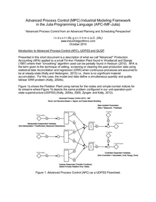
Presented in this short document is a description of what is well-known as Advanced Process Control (APC) applied to a small linear three (3) manipulated variable (MV) by two (2) controlled variable (CV) problem. These problems are also known as Model Predictive Control (MPC) (Grimm et. al., 1989) and Moving Horizon Control (MHC). Figure 1 shows the 3 x 2 APC problem configured in our unit-operation-port-state superstructure (UOPSS) (Kelly, 2004, 2005; Zyngier and Kelly, 2012) as an Advanced Planning and Scheduling (APS) problem as opposed to a traditional APC problem. Although there is a tremendous amount of stability, performance and robustness theory associated with APC which can be directly assumed to APS problems (Mastragostino et. al., 2014), our approach is to show that APC can equally be set into an APS framework except that APS has far less sensitivity technology due to its inherent discrete and nonlinear modeling complexities i.e., especially non-convexities. In order to eliminate the steady-state offset between the actual value and its target, it is well-known to apply bias-updating though other forms of “parameter-feedback” is possible. Typically, APS applications only employ “variable-feedback” i.e., opening or initial inventories, properties, etc. but this alone will not alleviate the steady-state offset as demonstrated by Kelly and Zyngier (2008).

1. Advanced Process Control (MPC) Industrial Modeling Framework
in the Julia Programming Language (APC-IMF-Julia)
“Advanced Process Control from an Advanced Planning and Scheduling Perspective”
i n d u s t r IAL g o r i t h m s LLC. (IAL)
www.industrialgorithms.com
October 2014
Introduction to Advanced Process Control (APC), UOPSS and QLQP
Presented in this short document is a description of what is well-known as Advanced Process
Control (APC) applied to a small linear three (3) manipulated variable (MV) by two (2) controlled
variable (CV) problem. These problems are also known as Model Predictive Control (MPC)
(Grimm et. al., 1989) and Moving Horizon Control (MHC). Figure 1 shows the 3 x 2 APC
problem configured in our unit-operation-port-state superstructure (UOPSS) (Kelly, 2004, 2005;
Zyngier and Kelly, 2012) as an Advanced Planning and Scheduling (APS) problem as opposed
to a traditional APC problem.
Although there is a tremendous amount of stability, performance and robustness theory
associated with APC which can be directly assumed to APS problems (Mastragostino et. al.,
2014), our approach is to show that APC can equally be set into an APS framework except that
APS has far less sensitivity technology due to its inherent discrete and nonlinear modeling
complexities i.e., especially non-convexities. In order to eliminate the steady-state offset
between the actual value and its target, it is well-known to apply bias-updating though other
forms of “parameter-feedback” is possible. Typically, APS applications only employ “variable-
feedback” i.e., opening or initial inventories, properties, etc. but this alone will not alleviate the
steady-state offset as demonstrated by Kelly and Zyngier (2008).
Figure 1. Advanced Process Control (APC) as a UOPSS Flowsheet.

2. The diamond shapes or objects are the sources and sinks known as perimeters, the rectangle
shapes without cross-hairs are batch-process units and the shapes with cross-hairs are
continuous-process units. The circle shapes with no cross-hairs are in-ports which can accept
one or more inlet flows and are considered to be simple or uncontrolled mixers. The cross-
haired circles are out-ports which can allow one or more outlet flows and are considered to be
simple or uncontrolled splitters. The lines, arcs or edges in between the various shapes or
structures are known as internal and external streams and represent in this context the flows or
transfers of materials from one shape to another.
In this formulation we do not use the manipulated variable “moves” (MV,t – MV,t-1) traditionally
found in Dynamic Matrix Control (DMC) for example but instead we use the actual MV values.
Each batch-process corresponds to one MV and has as many CV “states” as there are out-ports
configured. Given that we are not using MV moves, we use the finite impulse-response (FIR)
for each MV-CV pair as opposed to the step-response (SR). The interesting feature of this
implementation is our use of the batch-process with relative-time yield patterns or profiles
(Kondili et. al., 1993, Zyngier and Kelly, 2009) to model the ad hoc and relative-time-varying
nature of the FIR. This also allows for the pure delay, dead-time or lag where the FIR is set to
zero (0) for the initial relative-time-periods given that there is no appreciable CV response with
respect to the MV. Furthermore, in our formulation we also support the use of lower and upper
yield values for each relative-time-period which can be used to represent some level of
uncertainty, variation or distribution in the FIR i.e., from the FIR identification and parameter
estimation.
To describe in more detail our unique formulation highlighted in Figure 1, we have delineated
the five (5) stages of an Advanced Process Control (APC) problem modeled as an Advanced
Planning and Scheduling (APS) problem:
1. “Supply” the manipulated (independent/exogenous) variables which have lower and
upper hard bounds as well as target soft bounds (i.e., ideal or desired steady-state
values).
Non-manipulated variables are also independent/exogenous such as feedforward and
measured/unmeasured disturbance variables but have their lower, upper and target
bounds fixed i.e., they are not manipulatable.
2. “Process” (transform, transfer) the manipulated variables into controlled
(dependent/endogenous) variable states modeled as batch-processes with relative-time
yields representing the finite impulse-responses (FIR). If we were to use manipulated
variable moves (temporal deviations) then we would replace the FIR curve with a SR
curve.
For open-loop stable or self-regulating (minimum-phase) processes, the impulse-
response resembles a delayed monotonic decaying, declining or degrading process
yield profile and eventually goes to zero (0). For non-minimum phase processes the
impulse-response or yield profile will be non-monotonic with at least one extreme point.
For integrating processes such as holdup or inventory processes, the impulse-response
coefficient will settle to a non-zero constant.
3. “Sum” (superimpose) the controlled variable states, or contributions from each
manipulated variable, to yield a composite or total controlled variable prediction.

3. 4. “Bias” update (estimate) and augment the controlled variable’s prediction using a bias
parameter or coefficient computed using the actual or measured controlled variable’s
current value minus its previous prediction value for the same time-period/interval from
the last iteration, cycle or execution of the controller. The bias parameter is an estimate
over time of the uncertainty or mismatch between what is known and what is unknown in
the system.
If there is no measurement feedback such as in an off-line simulation or the meter,
instrument, device or analyzer is mal-functioning, then the bias equals zero (0).
Conversely, if a manipulated variable has failed or is saturated, then it can be easily
fixed to its existing value by configuring its lower and upper bounds to be the same.
Other advanced parameter updating techniques known as Moving Horizon Estimation
(MHE) can also be used but this requires Nonlinear Dynamic Data Reconciliation and
Regression (NDDRR) techniques with hopefully rich data in order to observe both
structurally and statistically all of the updated or real-time/on-line coefficients. With this
type of on-line or real-time estimation puts the strategy into the class of adaptive control.
5. “Demand” (control, command) the level, amount or activity of each controlled variable
required to fulfill the necessary requirements of the controller considering both the
upstream and downstream integration of the process and/or production. The activity is
managed using the lower, upper and target bounds which can be time-varying within the
controller’s prediction time-horizon.
It should be noted that for bias-updating an explicit biasing stage or step is not required
given that the bias can be simply subtracted from the controlled variable’s target,
setpoint or reference value.
Industrial Modeling Framework (IMF), IMPL and SSIIMPLE
To implement the mathematical formulation of this and other systems, IAL offers a unique
approach and is incorporated into our Industrial Modeling Programming Language we call IMPL.
IMPL has its own modeling language called IML (short for Industrial Modeling Language) which
is a flat or text-file interface as well as a set of API's which can be called from any computer
programming language such as C, C++, Fortran, C#, VBA, Java (SWIG), Python (CTYPES)
and/or Julia (CCALL) called IPL (short for Industrial Programming Language) to both build the
model and to view the solution. Models can be a mix of linear, mixed-integer and nonlinear
variables and constraints and are solved using a combination of LP, QP, MILP and NLP solvers
such as COINMP, GLPK, LPSOLVE, SCIP, CPLEX, GUROBI, LINDO, XPRESS, CONOPT,
IPOPT, KNITRO and WORHP as well as our own implementation of SLP called SLPQPE
(Successive Linear & Quadratic Programming Engine) which is a very competitive alternative to
the other nonlinear solvers and embeds all available LP and QP solvers.
In addition and specific to DRR problems, we also have a special solver called SECQPE
standing for Sequential Equality-Constrained QP Engine which computes the least-squares
solution and a post-solver called SORVE standing for Supplemental Observability, Redundancy
and Variability Estimator to estimate the usual DRR statistics. SECQPE also includes a
Levenberg-Marquardt regularization method for nonlinear data regression problems and can be
presolved using SLPQPE i.e., SLPQPE warm-starts SECQPE. SORVE is run after the
SECQPE solver and also computes the well-known "maximum-power" gross-error statistics

4. (measurement and nodal/constraint tests) to help locate outliers, defects and/or faults i.e., mal-
functions in the measurement system and mis-specifications in the logging system.
The underlying system architecture of IMPL is called SSIIMPLE (we hope literally) which is short
for Server, Solvers, Interfacer (IML), Interacter (IPL), Modeler, Presolver Libraries and
Executable. The Server, Solvers, Presolver and Executable are primarily model or problem-
independent whereas the Interfacer, Interacter and Modeler are typically domain-specific i.e.,
model or problem-dependent. Fortunately, for most industrial planning, scheduling,
optimization, control and monitoring problems found in the process industries, IMPL's standard
Interfacer, Interacter and Modeler are well-suited and comprehensive to model the most difficult
of production and process complexities allowing for the formulations of straightforward
coefficient equations, ubiquitous conservation laws, rigorous constitutive relations, empirical
correlative expressions and other necessary side constraints.
User, custom, adhoc or external constraints can be augmented or appended to IMPL when
necessary in several ways. For MILP or logistics problems we offer user-defined constraints
configurable from the IML file or the IPL code where the variables and constraints are
referenced using unit-operation-port-state names and the quantity-logic variable types. It is also
possible to import a foreign *.ILP file (row-based MPS file) which can be generated by any
algebraic modeling language or matrix generator. This file is read just prior to generating the
matrix and before exporting to the LP, QP or MILP solver. For NLP or quality problems we offer
user-defined formula configuration in the IML file and single-value and multi-value function
blocks writable in C, C++ or Fortran. The nonlinear formulas may include intrinsic functions
such as EXP, LN, LOG, SIN, COS, TAN, MIN, MAX, IF, NOT, EQ, NE, LE, LT, GE, GT and CIP,
LIP, SIP and KIP (constant, linear and monotonic spline interpolations) as well as user-written
extrinsic functions (XFCN). It is also possible to import another type of foreign file called the
*.INL file where both linear and nonlinear constraints can be added easily using new or existing
IMPL variables.
Industrial modeling frameworks or IMF's are intended to provide a jump-start to an industrial
project implementation i.e., a pre-project if you will, whereby pre-configured IML files and/or IPL
code are available specific to your problem at hand. The IML files and/or IPL code can be
easily enhanced, extended, customized, modified, etc. to meet the diverse needs of your project
and as it evolves over time and use. IMF's also provide graphical user interface prototypes for
drawing the flowsheet as in Figure 1 and typical Gantt charts and trend plots to view the solution
of quantity, logic and quality time-profiles. Current developments use Python 2.3 and 2.7
integrated with open-source Gnome Dia and Matplotlib modules respectively but other
prototypes embedded within Microsoft Excel/VBA for example can be created in a
straightforward manner.
However, the primary purpose of the IMF's is to provide a timely, cost-effective, manageable
and maintainable deployment of IMPL to formulate and optimize complex industrial
manufacturing systems in either off-line or on-line environments. Using IMPL alone would be
somewhat similar (but not as bad) to learning the syntax and semantics of an AML as well as
having to code all of the necessary mathematical representations of the problem including the
details of digitizing your data into time-points and periods, demarcating past, present and future
time-horizons, defining sets, index-sets, compound-sets to traverse the network or topology,
calculating independent and dependent parameters to be used as coefficients and bounds and
finally creating all of the necessary variables and constraints to model the complex details of
logistics and quality industrial optimization problems. Instead, IMF's and IMPL provide, in our

5. opinion, a more elegant and structured approach to industrial modeling and solving so that you
can capture the benefits of advanced decision-making faster, better and cheaper.
Advanced Process Control (Model Predictive Control/Moving Horizon Control) Synopsis
At this point we explore further the application of APS to model and solve the 3 x 2 APC
problem found in Figure 1. Appendices A and B show the UPS and IML files respectively where
the IML files contains the FIR configuration found in the “Constriction Data” (see the keyword
LIP which stands for linear (monotonic) interpolation). There are six (3 x 2 = 6) FIR’s which are
identical in sizings except for changes in signs. For example, the FIR for CV1 w.r.t. MV1 is 0.0,
1.0, 0.5, 0.25, 0.0, … 0.0 for relative-time-periods 0, 1, 2, 3, 4, …, 90. Relative-time-period 0
will always be zero (0.0) given that for discrete sampled systems it will be impossible for the
MV’s to affect the CV’s at the zero instant or interval of time. It should be noted that it is
possible to configure both lower and upper bounds for the FIR’s which can be used to manage
uncertainty in the FIR identification and estimation as mentioned previously.
Appendix C provides the Julia code necessary to call IMPL including the calls to our IPL
routines. Julia is a relatively new and fast scientific computing programming language that is
open-source and is similar to Mathwork’s Matlab but is free. Julia allows the user to call C and
Fortran compiled DLL’s and SO’s that can be embedded seamlessly using its ccall()
functionality which we use extensively. Note that Julia wrappers could be easily written to make
the IMPL ccall()’s simpler for the user to call.
For this problem we set the past/present time-horizon to be ten (10) time-periods and the future
time-horizon to be also ten (10) time-periods with the latter known as the “prediction-horizon” in
MPC terminology (Grimm et. al., 1989). There can also be a “control-horizon” but we have
chosen for this to be identical to the prediction-horizon. The number of simulation intervals is
set at fifty (50) and we make setpoint or target changes of -1.0 for CV1 and 1.0 for CV2 at
simulation interval one (1) and are configured in IPL using the IPL routine
IMPLreceiveUOPSrateorder(). To implement the variable-feedback, we use the routine
IMPLreceiveUOholdupopen() which configures the past/present values for the MV values as
batch-process holdup openings (or batch-size initial-conditions). To implement the parameter-
feedback, we also use the routine IMPLreceiveUOPSrateorder()similar to the target/setpoint CV
orders except that we assume the CV1 and CV2 biases are both zero (0.0) and fix the lower
and upper bounds to this value i.e., we are assuming the FIR model is perfect.
With regards to the CV and MV weightings, the routines IMPLreceiveUOPSflowweight() and
IMPLreceiveUOholdupsmooth() are used respectively. The flow weight routine provides the 2-
norm weight in the weight * (CV,t – CV,t,Target)^2 QP objective function term and the holdup
smoothing routine provides the 2-norm weight in the weight * (MV,t – MV,t-1)^2 term also known
as “move-suppression”. These are also implemented to achieve what is known as “dynamic-
tuning” given that the controller is re-computed for each simulation instance. Figures 2a and 2b
highlight the MV’s and CV’s respectively using the Julia package called Winston where the QP
solver used is IBM’s CPLEX 12.6 with each simulation interval taking 0.035-seconds of
computer-time for this small 3 x 2 APC type of problem using an APS strategy.

6. Figure 2a. MV1 (Blue Triangles), MV2 (Green Stars) and MV3 (Magenta Pluses) Responses.
Figure 2b. CV1 (Blue Triangles) and CV2 (Green Stars) Responses.

7. In summary, we have highlighted the use IMPL to model and solve a small linear 3 x 2 APC
problem in an APS optimization framework coded in the computer programming language Julia.
The results would be identical to the same problem being modeled and solved using other APC
technology and software. The step-responses are replaced by finite impulse-responses
configured into IMPL’s batch-processes with relative-time-varying yields where these yields can
be contained between arbitrary lower and upper bounds to mitigate model mismatch for
example. Finally, one of the primary reasons to show that APS is functionally the same as APC
is to bring together these two disciplines in order to increase the spread or coverage of applying
industrial optimization technologies with the hopes of increasing the benefits that these
technologies provide collectively to the process industries.
References
Grimm, W.M., Lee, P.L., Callahan, P.J., “Practical robust predictive control of a heat exchange
network”, Chemical Engineering Communications, 81, 25-53, (1989).
Kondili, E., Pantelides, C.C., Sargent, R.W.H., “A general algorithm for the short-term
scheduling of batch operations – I MILP formulation”, Computers and Chemical Engineering, 17,
211, (1993).
Kelly, J.D., "Production modeling for multimodal operations", Chemical Engineering Progress,
February, 44, (2004).
Kelly, J.D., "The unit-operation-stock superstructure (UOSS) and the quantity-logic-quality
paradigm (QLQP) for production scheduling in the process industries", In: MISTA 2005
Conference Proceedings, 327, (2005).
Kelly, J.D., Zyngier, D., "Continuously improve planning and scheduling models with parameter
feedback", FOCAPO 2008, July, (2008).
Zyngier, D., Kelly, J.D., "Multi-product inventory logistics modeling in the process industries", In:
W. Chaovalitwonse, K.C. Furman and P.M. Pardalos, Eds., Optimization and Logistics
Challenges in the Enterprise", Springer, 61-95, (2009).
Zyngier, D., Kelly, J.D., "UOPSS: a new paradigm for modeling production planning and
scheduling systems", ESCAPE 22, June, (2012).
Mastragostino, R., Patel, S., Swartz, C.L.E., “Robust decision making for hybrid process supply
chains via model predictive control”, Computers and Chemical Engineering, 62, 37-55, (2014).
Appendix A – APC-IMF.UPS (UOPSS) File
i M P l (c)
Copyright and Property of i n d u s t r I A L g o r i t h m s LLC.
!!!!!!!!!!!!!!!!!!!!!!!!!!!!!!!!!!!!!!!!!!!!!!!!!!!!!!!!!!!!!!
! Unit-Operation-Port-State-Superstructure (UOPSS) *.UPS File.
! (This file is automatically generated from the Python program IALConstructer.py)
!!!!!!!!!!!!!!!!!!!!!!!!!!!!!!!!!!!!!!!!!!!!!!!!!!!!!!!!!!!!!!
&sUnit,&sOperation,@sType,@sSubtype,@sUse
CV1Bias,,perimeter,,
CV1Demand,,perimeter,,
CV1Sum,,processc,,
CV2Bias,,perimeter,,
CV2Demand,,perimeter,,
CV2Sum,,processc,,
MV1Process,,processb,,
MV1Supply,,perimeter,,

8. MV2Process,,processb,,
MV2Supply,,perimeter,,
MV3Process,,processb,,
MV3Supply,,perimeter,,
&sUnit,&sOperation,@sType,@sSubtype,@sUse
! Number of UO shapes = 12
&sAlias,&sUnit,&sOperation
ALLPARTS,CV1Bias,
ALLPARTS,CV1Demand,
ALLPARTS,CV1Sum,
ALLPARTS,CV2Bias,
ALLPARTS,CV2Demand,
ALLPARTS,CV2Sum,
ALLPARTS,MV1Process,
ALLPARTS,MV1Supply,
ALLPARTS,MV2Process,
ALLPARTS,MV2Supply,
ALLPARTS,MV3Process,
ALLPARTS,MV3Supply,
&sAlias,&sUnit,&sOperation
&sUnit,&sOperation,&sPort,&sState,@sType,@sSubtype
CV1Bias,,o,,out,
CV1Demand,,i,,in,
CV1Sum,,i,,in,
CV1Sum,,o,,out,
CV2Bias,,o,,out,
CV2Demand,,i,,in,
CV2Sum,,i,,in,
CV2Sum,,o,,out,
MV1Process,,i,,in,
MV1Process,,o1,,out,
MV1Process,,o2,,out,
MV1Supply,,o,,out,
MV2Process,,i,,in,
MV2Process,,o1,,out,
MV2Process,,o2,,out,
MV2Supply,,o,,out,
MV3Process,,i,,in,
MV3Process,,o1,,out,
MV3Process,,o2,,out,
MV3Supply,,o,,out,
&sUnit,&sOperation,&sPort,&sState,@sType,@sSubtype
! Number of UOPS shapes = 20
&sAlias,&sUnit,&sOperation,&sPort,&sState
ALLINPORTS,CV1Demand,,i,
ALLINPORTS,CV1Sum,,i,
ALLINPORTS,CV2Demand,,i,
ALLINPORTS,CV2Sum,,i,
ALLINPORTS,MV1Process,,i,
ALLINPORTS,MV2Process,,i,
ALLINPORTS,MV3Process,,i,
ALLOUTPORTS,CV1Bias,,o,
ALLOUTPORTS,CV1Sum,,o,
ALLOUTPORTS,CV2Bias,,o,
ALLOUTPORTS,CV2Sum,,o,
ALLOUTPORTS,MV1Process,,o1,
ALLOUTPORTS,MV1Process,,o2,
ALLOUTPORTS,MV1Supply,,o,
ALLOUTPORTS,MV2Process,,o1,
ALLOUTPORTS,MV2Process,,o2,
ALLOUTPORTS,MV2Supply,,o,
ALLOUTPORTS,MV3Process,,o1,
ALLOUTPORTS,MV3Process,,o2,
ALLOUTPORTS,MV3Supply,,o,
&sAlias,&sUnit,&sOperation,&sPort,&sState
&sUnit,&sOperation,&sPort,&sState,&sUnit,&sOperation,&sPort,&sState
CV1Bias,,o,,CV1Demand,,i,
CV1Sum,,o,,CV1Demand,,i,
CV2Bias,,o,,CV2Demand,,i,
CV2Sum,,o,,CV2Demand,,i,
MV1Process,,o1,,CV1Sum,,i,
MV1Process,,o2,,CV2Sum,,i,
MV1Supply,,o,,MV1Process,,i,
MV2Process,,o1,,CV1Sum,,i,
MV2Process,,o2,,CV2Sum,,i,
MV2Supply,,o,,MV2Process,,i,
MV3Process,,o1,,CV1Sum,,i,
MV3Process,,o2,,CV2Sum,,i,
MV3Supply,,o,,MV3Process,,i,
&sUnit,&sOperation,&sPort,&sState,&sUnit,&sOperation,&sPort,&sState
! Number of UOPSPSUO shapes = 13
&sAlias,&sUnit,&sOperation,&sPort,&sState,&sUnit,&sOperation,&sPort,&sState
ALLPATHS,CV1Bias,,o,,CV1Demand,,i,
ALLPATHS,CV1Sum,,o,,CV1Demand,,i,
ALLPATHS,MV1Process,,o1,,CV1Sum,,i,
ALLPATHS,MV2Process,,o1,,CV1Sum,,i,
ALLPATHS,MV3Process,,o1,,CV1Sum,,i,

9. ALLPATHS,CV2Bias,,o,,CV2Demand,,i,
ALLPATHS,CV2Sum,,o,,CV2Demand,,i,
ALLPATHS,MV1Process,,o2,,CV2Sum,,i,
ALLPATHS,MV2Process,,o2,,CV2Sum,,i,
ALLPATHS,MV3Process,,o2,,CV2Sum,,i,
ALLPATHS,MV1Supply,,o,,MV1Process,,i,
ALLPATHS,MV2Supply,,o,,MV2Process,,i,
ALLPATHS,MV3Supply,,o,,MV3Process,,i,
&sAlias,&sUnit,&sOperation,&sPort,&sState,&sUnit,&sOperation,&sPort,&sState
Appendix B – APC-IMF.IML File
i M P l (c)
Copyright and Property of i n d u s t r I A L g o r i t h m s LLC.
!!!!!!!!!!!!!!!!!!!!!!!!!!!!!!!!!!!!!!!!!!!!!!!!!!!!!!!!!!!!!!!!!!!!!!!!!!!!!!!!
! Calculation Data (Parameters)
!!!!!!!!!!!!!!!!!!!!!!!!!!!!!!!!!!!!!!!!!!!!!!!!!!!!!!!!!!!!!!!!!!!!!!!!!!!!!!!!
&sCalc,@sValue
START,-100.0
BEGIN,0.0
END,100.0
PERIOD,1.0
LARGE,10000.0
&sCalc,@sValue
!!!!!!!!!!!!!!!!!!!!!!!!!!!!!!!!!!!!!!!!!!!!!!!!!!!!!!!!!!!!!!!!!!!!!!!!!!!!!!!!
! Chronological Data (Periods)
!!!!!!!!!!!!!!!!!!!!!!!!!!!!!!!!!!!!!!!!!!!!!!!!!!!!!!!!!!!!!!!!!!!!!!!!!!!!!!!!
@rPastTHD,@rFutureTHD,@rTPD
START,END,PERIOD
@rPastTHD,@rFutureTHD,@rTPD
!!!!!!!!!!!!!!!!!!!!!!!!!!!!!!!!!!!!!!!!!!!!!!!!!!!!!!!!!!!!!!!!!!!!!!!!!!!!!!!!
! Construction Data (Pointers)
!!!!!!!!!!!!!!!!!!!!!!!!!!!!!!!!!!!!!!!!!!!!!!!!!!!!!!!!!!!!!!!!!!!!!!!!!!!!!!!!
Include-@sFile_Name
APC-IMF.ups
Include-@sFile_Name
!!!!!!!!!!!!!!!!!!!!!!!!!!!!!!!!!!!!!!!!!!!!!!!!!!!!!!!!!!!!!!!!!!!!!!!!!!!!!!!!
! Capacity Data (Prototypes)
!!!!!!!!!!!!!!!!!!!!!!!!!!!!!!!!!!!!!!!!!!!!!!!!!!!!!!!!!!!!!!!!!!!!!!!!!!!!!!!!
&sUnit,&sOperation,@rRate_Lower,@rRate_Upper
CV1Sum,,-LARGE,LARGE
CV2Sum,,-LARGE,LARGE
&sUnit,&sOperation,@rRate_Lower,@rRate_Upper
&sUnit,&sOperation,@rHoldup_Lower,@rHoldup_Upper
MV1Process,,-LARGE,LARGE
MV2Process,,-LARGE,LARGE
MV3Process,,-LARGE,LARGE
&sUnit,&sOperation,@rHoldup_Lower,@rHoldup_Upper
&sUnit,&sOperation,&sPort,&sState,@rTeeRate_Lower,@rTeeRate_Upper
ALLINPORTS,-LARGE,LARGE
ALLOUTPORTS,-LARGE,LARGE
&sUnit,&sOperation,&sPort,&sState,@rTeeRate_Lower,@rTeeRate_Upper
&sUnit,&sOperation,&sPort,&sState,@rTotalRate_Lower,@rTotalRate_Upper
ALLINPORTS,-LARGE,LARGE
ALLOUTPORTS,-LARGE,LARGE
&sUnit,&sOperation,&sPort,&sState,@rTotalRate_Lower,@rTotalRate_Upper
&sUnit,&sOperation,&sPort,&sState,@rYield_Lower,@rYield_Upper,@rYield_Fixed
MV1Process,,i,,1.0,1.0
MV2Process,,i,,1.0,1.0
MV3Process,,i,,1.0,1.0
MV1Process,,o1,,0.0,0.0
MV1Process,,o2,,0.0,0.0
MV2Process,,o1,,0.0,0.0
MV2Process,,o2,,0.0,0.0
MV3Process,,o1,,0.0,0.0
MV3Process,,o2,,0.0,0.0
CV1Sum,,i,,1.0,1.0
CV1Sum,,o,,1.0,1.0
CV2Sum,,i,,1.0,1.0
CV2Sum,,o,,1.0,1.0
&sUnit,&sOperation,&sPort,&sState,@rYield_Lower,@rYield_Upper,@rYield_Fixed
!!!!!!!!!!!!!!!!!!!!!!!!!!!!!!!!!!!!!!!!!!!!!!!!!!!!!!!!!!!!!!!!!!!!!!!!!!!!!!!!
! Constriction Data (Practices/Policies)
!!!!!!!!!!!!!!!!!!!!!!!!!!!!!!!!!!!!!!!!!!!!!!!!!!!!!!!!!!!!!!!!!!!!!!!!!!!!!!!!
&sUnit,&sOperation,@rUpTiming_Lower,@rUpTiming_Upper
MV1Process,,1.0,1.0
MV2Process,,1.0,1.0
MV3Process,,1.0,1.0

10. &sUnit,&sOperation,@rUpTiming_Lower,@rUpTiming_Upper
&sUnit,&sOperation,&sPort,&sState,@rFlowDelaying_Lower,@rFlowDelaying_Upper
MV1Process,,o1,,0.0,90.0
MV1Process,,o2,,0.0,90.0
MV2Process,,o1,,0.0,90.0
MV2Process,,o2,,0.0,90.0
MV3Process,,o1,,0.0,90.0
MV3Process,,o2,,0.0,90.0
&sUnit,&sOperation,&sPort,&sState,@rFlowDelaying_Lower,@rFlowDelaying_Upper
&sUnit,&sOperation,&sPort,&sState,@rYieldDelaying_Lower,@rYieldDelaying_Upper,@rInitial_Time,@sType
MV1Process,,o1,,0.0,0.0,0.0,LIP
MV1Process,,o1,,1.0,1.0,1.0,LIP
MV1Process,,o1,,0.5,0.5,2.0,LIP
MV1Process,,o1,,0.25,0.25,3.0,LIP
MV1Process,,o1,,0.0,0.0,4.0,LIP
MV1Process,,o1,,0.0,0.0,90.0,LIP
MV1Process,,o2,,0.0,0.0,0.0,LIP
MV1Process,,o2,,-1.0,-1.0,1.0,LIP
MV1Process,,o2,,-0.5,-0.5,2.0,LIP
MV1Process,,o2,,-0.25,-0.25,3.0,LIP
MV1Process,,o2,,0.0,0.0,4.0,LIP
MV1Process,,o2,,0.0,0.0,90.0,LIP
MV2Process,,o1,,0.0,0.0,0.0,LIP
MV2Process,,o1,,-1.0,-1.0,1.0,LIP
MV2Process,,o1,,-0.5,-0.5,2.0,LIP
MV2Process,,o1,,-0.25,-0.25,3.0,LIP
MV2Process,,o1,,0.0,0.0,4.0,LIP
MV2Process,,o1,,0.0,0.0,90.0,LIP
MV2Process,,o2,,0.0,0.0,0.0,LIP
MV2Process,,o2,,1.0,1.0,1.0,LIP
MV2Process,,o2,,0.5,0.5,2.0,LIP
MV2Process,,o2,,0.25,0.25,3.0,LIP
MV2Process,,o2,,0.0,0.0,4.0,LIP
MV2Process,,o2,,0.0,0.0,90.0,LIP
MV3Process,,o1,,0.0,0.0,0.0,LIP
MV3Process,,o1,,1.0,1.0,1.0,LIP
MV3Process,,o1,,0.5,0.5,2.0,LIP
MV3Process,,o1,,0.25,0.25,3.0,LIP
MV3Process,,o1,,0.0,0.0,4.0,LIP
MV3Process,,o1,,0.0,0.0,90.0,LIP
MV3Process,,o2,,0.0,0.0,0.0,LIP
MV3Process,,o2,,1.0,1.0,1.0,LIP
MV3Process,,o2,,0.5,0.5,2.0,LIP
MV3Process,,o2,,0.25,0.25,3.0,LIP
MV3Process,,o2,,0.0,0.0,4.0,LIP
MV3Process,,o2,,0.0,0.0,90.0,LIP
&sUnit,&sOperation,&sPort,&sState,@rYieldDelaying_Lower,@rYieldDelaying_Upper,@rInitial_Time,@sType
MV1Process,,,1.0
MV2Process,,,1.0
MV3Process,,,1.0
&sUnit,&sOperation,@rHoldupSmoothing1_Weight,@rHoldupSmoothing2_Weight
&sUnit,&sOperation,@rHoldupSmoothing1_Weight,@rHoldupSmoothing2_Weight
!!!!!!!!!!!!!!!!!!!!!!!!!!!!!!!!!!!!!!!!!!!!!!!!!!!!!!!!!!!!!!!!!!!!!!!!!!!!!!!!
! Cost Data (Pricing)
!!!!!!!!!!!!!!!!!!!!!!!!!!!!!!!!!!!!!!!!!!!!!!!!!!!!!!!!!!!!!!!!!!!!!!!!!!!!!!!!
CV1Demand,,i,,,,1.0,
CV2Demand,,i,,,,1.0,
&sUnit,&sOperation,&sPort,&sState,@rFlowPro_Weight,@rFlowPer1_Weight,@rFlowPer2_Weight,@rFlowPen_Weight
&sUnit,&sOperation,&sPort,&sState,@rFlowPro_Weight,@rFlowPer1_Weight,@rFlowPer2_Weight,@rFlowPen_Weight
!!!!!!!!!!!!!!!!!!!!!!!!!!!!!!!!!!!!!!!!!!!!!!!!!!!!!!!!!!!!!!!!!!!!!!!!!!!!!!!!
! Content Data (Past, Present Provisos)
!!!!!!!!!!!!!!!!!!!!!!!!!!!!!!!!!!!!!!!!!!!!!!!!!!!!!!!!!!!!!!!!!!!!!!!!!!!!!!!!
MV1Process,,0.0,-1.0
MV2Process,,0.0,-1.0
MV3Process,,0.0,-1.0
&sUnit,&sOperation,@rHoldup_Value,@rStart_Time
&sUnit,&sOperation,@rHoldup_Value,@rStart_Time
!!!!!!!!!!!!!!!!!!!!!!!!!!!!!!!!!!!!!!!!!!!!!!!!!!!!!!!!!!!!!!!!!!!!!!!!!!!!!!!!
! Command Data (Future Provisos)
!!!!!!!!!!!!!!!!!!!!!!!!!!!!!!!!!!!!!!!!!!!!!!!!!!!!!!!!!!!!!!!!!!!!!!!!!!!!!!!!
&sUnit,&sOperation,@rSetup_Lower,@rSetup_Upper,@rBegin_Time,@rEnd_Time
ALLPARTS,1,1,BEGIN,END
&sUnit,&sOperation,@rSetup_Lower,@rSetup_Upper,@rBegin_Time,@rEnd_Time
&sUnit,&sOperation,@rStartup_Lower,@rStartup_Upper,@rBegin_Time,@rEnd_Time
MV1Process,,1,1,BEGIN,END
MV2Process,,1,1,BEGIN,END
MV3Process,,1,1,BEGIN,END
&sUnit,&sOperation,@rStartup_Lower,@rStartup_Upper,@rBegin_Time,@rEnd_Time
&sUnit,&sOperation,&sPort,&sState,&sUnit,&sOperation,&sPort,&sState,@rSetup_Lower,@rSetup_Upper,@rBegin_Time,@rEnd_Time
ALLPATHS,1,1,BEGIN,END
&sUnit,&sOperation,&sPort,&sState,&sUnit,&sOperation,&sPort,&sState,@rSetup_Lower,@rSetup_Upper,@rBegin_Time,@rEnd_Time
CV1Demand,,i,,-100.0,100.0,0.0,BEGIN,END
CV2Demand,,i,,-100.0,100.0,0.0,BEGIN,END

11. CV1Bias,,o,,0.0,0.0,,BEGIN,END
CV2Bias,,o,,0.0,0.0,,BEGIN,END
&sUnit,&sOperation,&sPort,&sState,@rTotalRate_Lower,@rTotalRate_Upper,@rTotalRate_Target,@rBegin_Time,@rEnd_Time
&sUnit,&sOperation,&sPort,&sState,@rTotalRate_Lower,@rTotalRate_Upper,@rTotalRate_Target,@rBegin_Time,@rEnd_Time
Appendix C – APC-IMF-Julia.JL File
###############################################################################
# INDUSTRIAL ALGORITHMS LLC. CONFIDENTIAL & PROPRIETARY #######################
###############################################################################
#
# File: IMPLjulia.jl
#
# Author: Jeffrey D. Kelly
# Date: September 21, 2014
# Language: Julia.
#
# Program Description:
#
# This program embeds IMPL into Julia using its ccall() functionality to perform
# a closed-loop advanced process control (APC) simulation of a small linear model
# predictive control (MPC) or moving horizon control (MHC) problem.
#
# This program highlights the difference between "variable-feedback" and "parameter-
# feedback" (Kelly and Zyngier, 2008). Variable-feedback is measurement-feedback
# using the measured independent and dependent variables values as openings,
# starting-values or initial-conditions. Parameter-feedback is also measurement-
# feedback but involves calculating parameters or coefficients using either data
# reconciliation and regression (DRR) or simple bias-updating (see moving horizon
# estimation (MHE)). Without parameter-feedback, steady-state offsets will occur
# with omni-present model-mismatch or uncertainty i.e., non-zero differences between
# the setpoint, reference or target from the actual or measured controlled variable values.
#
# The reason for delineating the differences between variable and parameter-
# feedback is to demonstrate that in advanced planning and scheduling (APS)
# applications, if variable-feedback alone is used (via opening values only) without
# parameter-feedback as used in advanced process control (APC) with at least bias-updating,
# then significant actual versus plan/schedule deviations, deltas or offsets will occur
# (Kelly and Zyngier, 2008) due to the unmanaged uncertainties in the system.
#
# References:
#
# Kelly, J.D., Zyngier, D., "Continuously improve planning and scheduling models with
# parameter feedback", FOCAPO 2008, July, (2008).
#
# Revision History:
#
# 1.0 J.D. Kelly, September 21, 2014
#
# Start date of program - Version 14.9.211
#
###############################################################################
# INDUSTRIAL ALGORITHMS LLC. CONFIDENTIAL & PROPRIETARY #######################
###############################################################################
# Use Winston as the Julia plotting module - see also ASCIIPlots and Gadfly.
using Winston
# Include the IMPL constants (see the IMPL.hdr file).
include("C:IndustrialAlgorithmsProgramsimpljuliainclude.jl")
# Set the path to where the IMPL shared objects (DLL's) are located.
cd("c:industrialalgorithmsplatformimpl")
#cd("c:impl")
# Set the IML file containing the "base" model-data. The "delta" model-data is set
# using IPL during the simulation loops, cycles or iterations.
#fact = "C:IndustrialAlgorithmsPortfolioAPC-IMF"
fact = "C:implapcAPC-IMF"
println(fact)
# Set and get the USELOGFILE setting.
setting = "USELOGFILE"
rtnstat = ccall( (:IMPLreceiveSETTING,"IMPLserver"), Cint, (Ptr{Uint8},Cdouble), setting,IMPLyes)
IMPLuselogfile = ccall( (:IMPLretrieveSETTING,"IMPLserver"), Cdouble, (Ptr{Uint8},), setting)
println("USELOGFILE = ",IMPLuselogfile)
# Initialize the environment and allocate the IMPL resource-entities i.e., sets, lists,
# catalogs, parameters, variables, constraints, derivatives, expressions and formulas.
rtnstat = ccall( (:IMPLroot,"IMPLserver"), Cint, (Ptr{Uint8},) ,fact)
rtnstat = ccall( (:IMPLreserve,"IMPLserver"), Cint, (Ptr{Uint8},Cint), fact,IMPLall)
# Get the RNNON setting.
setting = "RNNON"
IMPLrnnon = ccall( (:IMPLretrieveSETTING,"IMPLserver"), Cdouble, (Ptr{Uint8},), setting)
println("RNNON = ",IMPLrnnon)

12. # "Interface" to the base model-data using the IML file specified ("fact").
form = IMPLsparsic
#form = IMPLsymbolic
fit = IMPLdiscrete
filter = IMPLlogistics
focus = IMPLoptimization
face = IMPLimport
factor = IMPLscale
fob = IMPLsipherless
frames = string(char(0))
rtnstat = ccall( (:IMPLinterfaceri,"IMPLinterfaceri"), Cint, (Ptr{Uint8},Cint,Cint,Cint,Cint,Cint,Cdouble,Clonglong,Ptr{Uint8 }),
fact,form,fit,filter,focus,face,factor,fob,frames)
# Set the durations of past/present and future time-horizons and the time-period (discrete-time).
#
# * Note that the duration of the future time-horizon (dthf) is identical to the "prediction-horizon"
# and "control-horizon" found in model predictive control (MPC) theory.
dthp = -10.0
dthf = 10.0
dtp = 1.0
rtnstat = ccall( (:IMPLreceiveT,"IMPLinteracter"), Cint, (Cdouble,Cdouble,Cdouble),
dthp,dthf,dtp)
# "Serialize" the base model-data to a binary (unformatted) file which is faster to re-read than the IML
# (ASCII) flat-file.
#
# * Note that at this point we are establishing a base model-data which is over-loaded or incrementally
# modified during the closed-loop simulation by adding what IMPL calls "openings" and "orders" for the
# variable- and parameter-feedback.
rtnstat = ccall( (:IMPLrender,"IMPLserver"), Cint, (Ptr{Uint8},Cint), fact,IMPLall)
# Get the number of discretized time-periods in the past/present and future time-horizons.
NTP = int32(abs(dthp) / dtp)
NTF = int32(dthf / dtp)
# Set the number of closed-loop simulation intervals or iterations.
NSIM = 50
# Initialize the manipulated and controlled variable (MV and CV) solution vectors.
MV1 = zeros(Float64,NSIM+NTP)
MV2 = zeros(Float64,NSIM+NTP)
MV3 = zeros(Float64,NSIM+NTP)
CV1 = zeros(Float64,NSIM+NTP)
CV2 = zeros(Float64,NSIM+NTP)
# Initialize the controlled variable setpoint/reference/target scenarios.
CV1S = zeros(Float64,NSIM)
CV2S = zeros(Float64,NSIM)
for i = 1:NSIM
if i > 0
CV1S[i] = -1.0
end
if i > 0
CV2S[i] = 1.0
end
end
# Initialize the IMPL objective function terms which must be set as 1D arrays or vectors in
# Julia in order to return or retrieve values by-reference.
profit = Cdouble[0.0]
performance1 = Cdouble[0.0]
performance2 = Cdouble[0.0]
penalty = Cdouble[0.0]
total = Cdouble[0.0]
tic()
TI = zeros(Float64,NSIM)
for i = 1:NSIM
TI[i] = i
# Refresh the IMPL resource-entities and restore the base model-data from the previously rendered or
# serialized binary file.
rtnstat = ccall( (:IMPLrefresh,"IMPLserver"), Cint, (Cint,) ,IMPLall)
rtnstat = ccall( (:IMPLrestore,"IMPLserver"), Cint, (Ptr{Uint8},Cint), fact,IMPLall)
# * IMPORTANT NOTE * - Model-Data Configuration via ASCII/Flat-File (IML) and API/Callable Libraries (IPL).
#
# IMPL allows a mix of two methods to configure the static and dynamic model-data in any order. This is through
# IMPL's "interfacer" and the "interacter". The IMPLinterfacer() configures the model-data through the IML
# (Industrial Modeling Language) and the IMPLinteracter() configures the model-data through the IPL (Industrial
# Programming Language).
#

13. # This allows partial configuration using whatever method is convenient and prudent for th e user.
# Set the "variable-feedback" for the manipulated variables. This is also referred to as "initial-conditions"
# or "boundary-conditions" in ODE's and DAE's or "openings" in APS (Kelly and Zyngier, 2008).
oname = " "
status = IMPLkeep
for t = 1:NTP
uname = "MV1Process"
value = MV1[i+NTP-t]
starttime = -float64(t) * dtp
rtnstat = ccall( (:IMPLreceiveUOholdupopen,"IMPLinteracter"), Cint, (Ptr{Uint8},Ptr{Uint8},Cdouble,Cdouble,Cint),
uname,oname,value,starttime,status)
uname = "MV2Process"
value = MV2[i+NTP-t]
rtnstat = ccall( (:IMPLreceiveUOholdupopen,"IMPLinteracter"), Cint, (Ptr{Uint8},Ptr{Uint8},Cdouble,Cdouble,Cint),
uname,oname,value,starttime,status)
uname = "MV3Process"
value = MV3[i+NTP-t]
rtnstat = ccall( (:IMPLreceiveUOholdupopen,"IMPLinteracter"), Cint, (Ptr{Uint8},Ptr{Uint8},Cdouble,Cdouble,Cint),
uname,oname,value,starttime,status)
end
# Set the "orders" which set the lower, upper and target (setpoint/reference) bounds.
#
# * Note that these are flowrate orders or transaction as they represent a flow of stock, goods,
# resources or signals.
uname = "CV1Demand"
oname = " "
pname = "i"
sname = " "
lower = -100.0
upper = 100.0
target = CV1S[i]
begintime = 0.0
endtime = dthf
rtnstat = ccall( (:IMPLreceiveUOPSrateorder,"IMPLinteracter"), Cint,
(Ptr{Uint8},Ptr{Uint8},Ptr{Uint8},Ptr{Uint8},Cdouble,Cdouble,Cdouble,Cdouble,Cdouble,Cint),
uname,oname,pname,sname,lower,upper,target,begintime,endtime,status)
uname = "CV2Demand"
target = CV2S[i]
rtnstat = ccall( (:IMPLreceiveUOPSrateorder,"IMPLinteracter"), Cint,
(Ptr{Uint8},Ptr{Uint8},Ptr{Uint8},Ptr{Uint8},Cdouble,Cdouble,Cdouble,Cdouble,Cdouble,Cint),
uname,oname,pname,sname,lower,upper,target,begintime,endtime,status)
# Set the orders which set the parameter-feedback biases.
#
# * Note that because we are not simulating the actual plant the biases are zero (0).
#
# * Note that it is also possible to simply bias the setpoints/reference/targets above when simple bias -updating
# is employed.
uname = "CV1Bias"
oname = " "
pname = "o"
sname = " "
lower = 0.0
upper = 0.0
target = IMPLrnnon
rtnstat = ccall( (:IMPLreceiveUOPSrateorder,"IMPLinteracter"), Cint,
(Ptr{Uint8},Ptr{Uint8},Ptr{Uint8},Ptr{Uint8},Cdouble,Cdouble,Cdouble,Cdouble,Cdouble,Cint),
uname,oname,pname,sname,lower,upper,target,begintime,endtime,status)
uname = "CV2Bias"
rtnstat = ccall( (:IMPLreceiveUOPSrateorder,"IMPLinteracter"), Cint,
(Ptr{Uint8},Ptr{Uint8},Ptr{Uint8},Ptr{Uint8},Cdouble,Cdouble,Cdouble,Cdouble,Cdouble,Cint),
uname,oname,pname,sname,lower,upper,target,begintime,endtime,status)
# Set the setpoint/reference/target 2-norm performance weight for the CV's.
#
# * Note that these 2-norm performance weights are "tuning" parameters found in other model predictive
# controllers such as DMC, etc.
uname = "CV1Demand"
pname = "i"
prowt = 0.0
per1wt = 0.0
per2wt = 1.0
penwt = 0.0
rtnstat = ccall( (:IMPLreceiveUOPSflowweight,"IMPLinteracter"), Cint,
(Ptr{Uint8},Ptr{Uint8},Ptr{Uint8},Ptr{Uint8},Cdouble,Cdouble,Cdouble,Cdouble,Cint),
uname,oname,pname,sname,prowt,per1wt,per2wt,penwt,status)
uname = "CV2Demand"
per2wt = 1.0
rtnstat = ccall( (:IMPLreceiveUOPSflowweight,"IMPLinteracter"), Cint,
(Ptr{Uint8},Ptr{Uint8},Ptr{Uint8},Ptr{Uint8},Cdouble,Cdouble,Cdouble,Cdouble,Cint),
uname,oname,pname,sname,prowt,per1wt,per2wt,penwt,status)

14. # Set the 2-norm performance weight for the MV's also known as "move-suppression". From an APS viewpoint or perspective we call
# this "smoothing" which minimizes the temporal deviations i.e., minimize weight * (dMV,t = MV,t - MV,t-1)^2.
#
# * Note that this is similar to "dynamic tuning" given that we changing the performance weights "on -line" during the simulation.
uname = "MV1Process"
per1wt = 0.0
per2wt = 1.0
rtnstat = ccall( (:IMPLreceiveUOholdupsmooth,"IMPLinteracter"), Cint, (Ptr{Uint8},Ptr{Uint8},Cdouble,Cdouble,Cint),
uname,oname,per1wt,per2wt,status)
uname = "MV2Process"
per1wt = 0.0
per2wt = 1.0
rtnstat = ccall( (:IMPLreceiveUOholdupsmooth,"IMPLinteracter"), Cint, (Ptr{Uint8},Ptr{Uint8},Cdouble,Cdouble,Cint),
uname,oname,per1wt,per2wt,status)
uname = "MV3Process"
per1wt = 0.0
per2wt = 1.0
rtnstat = ccall( (:IMPLreceiveUOholdupsmooth,"IMPLinteracter"), Cint, (Ptr{Uint8},Ptr{Uint8},Cdouble,Cdouble,Cint),
uname,oname,per1wt,per2wt,status)
# "Model" the problem by first creating the dependent sets, lists, catalogs and parameters, then the variables and
# finally the constraints.
#
# Since this problem is linear (with a quadratic objective function), the derivatives are also created with the
# constraints else if a nonlinear problem then only the sparsity-pattern is created and the derivatives are calculated
# simultaneoulsy during the solving.
filler = IMPLsupplementalless
foreign = IMPLsupplementaryless
force = IMPLparameter
rtnstat = ccall( (:IMPLmodelerv,"IMPLmodelerv"), Cint, (Ptr{Uint8},Cint,Cint,Cint,Cint,Ptr{Clonglong},Ptr{Uint8},Ptr{Cint}),
fact,form,fit,filter,focus,&filler,foreign,&force)
force = IMPLvariable
rtnstat = ccall( (:IMPLmodelerv,"IMPLmodelerv"), Cint, (Ptr{Uint8},Cint,Cint,Cint,Cint,Ptr{Clonglong},Ptr{Uint8},Ptr{Cint}),
fact,form,fit,filter,focus,&filler,foreign,&force)
force = IMPLconstraint
rtnstat = ccall( (:IMPLmodelerc,"IMPLmodelerc"), Cint, (Ptr{Uint8},Cint,Cint,Cint,Cint,Ptr{Clonglong},Ptr{Uint8},Ptr{Cint}),
fact,form,fit,filter,focus,&filler,foreign,&force)
# "Presolve and solve" the problem using either a commerical QP (CPLEX) or an open-source QP (IPOPT).
#
# * Note that the QP problem can also be solved by IMPL's SECQPE solver which ignores all of the inequality
# constraints and only respects equality constraints. Several basis factorization packages are also
# available including PARDISO from Intel's MKL which is parallelizable. This is the same solver used to
# data reconciliation and regression (DRR) problems.
factorizer = IMPLsemisolverless
fresh = IMPLfirstsession
flashback = IMPLflatfile
feedback = IMPLsummonsless
fork = IMPLcplex
# fork = IMPLipopt
# fork = IMPLslpqpecplex
# fork = IMPLsecqpey12m
# fork = IMPLsecqpenspiv
# fork = IMPLsecqpema28
# fork = IMPLsecqpepardiso
rtnstat = ccall( (:IMPLpresolver,"IMPLpresolver"), Cint, (Ptr{Uint8},Cint,Cint,Cint,Cint,Cint,Cint,Cint,Cint,Ptr{Int64}),
fact,form,fit,filter,focus,factorizer,fork,fresh,flashback,&feedback)
# Get the current manipulated variable (MV) solution values required by the "variable -feedback".
#
# When we use finite impulse-responses (discrete convolution model) with the batch-process's relative-time yields then the
# controlled variables are completely calculatable or determinable using the past/present manipulated variables only. If
# transfer functions are used which model the time-series using efficient rational polynomial quotients then both past/present
# manipulated (independent) and controlled (dependent) variables are required.
uname = "MV1Process"
oname = " "
MV1[i+NTP] = ccall( (:IMPLretrieveUOholdup1,"IMPLinteracter"), Cdouble, (Ptr{Uint8},Ptr{Uint8},Cin t,Cint,Cint),
uname,oname,NTP,NTF,-(1+NTP))
uname = "MV2Process"
MV2[i+NTP] = ccall( (:IMPLretrieveUOholdup1,"IMPLinteracter"), Cdouble, (Ptr{Uint8},Ptr{Uint8},Cint,Cint,Cint),
uname,oname,NTP,NTF,-(1+NTP))
uname = "MV3Process"
MV3[i+NTP] = ccall( (:IMPLretrieveUOholdup1,"IMPLinteracter"), Cdouble, (Ptr{Uint8},Ptr{Uint8},Cint,Cint,Cint),
uname,oname,NTP,NTF,-(1+NTP))
# Get the current controlled variable (CV) solution values required by both "parameter -feedback" and
# "variable-feedback" or bias-updating.
#
# * Note, given that we are only performing off-line simulation, there are no measured or actual values for
# the controlled variables so the biases are naturally zero (0) and we do not need to update these in the
# model-data using order or transactions.
#
# If this were an on-line situation with actual field or laboratory measurements at time t then we would take
# these CV measurements subtract them from the CV predictions at time t to compute the simple biases. These biases
# can then be subtracted from the setpoints, references or targets with the explicit bias flow streams.

15. uname = "CV1Demand"
oname = " "
pname = "i"
sname = " "
CV1[i+NTP] = ccall( (:IMPLretrieveUOPSflow1,"IMPLinteracter"), Cdouble,
(Ptr{Uint8},Ptr{Uint8},Ptr{Uint8},Ptr{Uint8},Cint,Cint,Cint),
uname,oname,pname,sname,NTP,NTF,-(1+NTP))
uname = "CV2Demand"
CV2[i+NTP] = ccall( (:IMPLretrieveUOPSflow1,"IMPLinteracter"), Cdouble,
(Ptr{Uint8},Ptr{Uint8},Ptr{Uint8},Ptr{Uint8},Cint,Cint,Cint),
uname,oname,pname,sname,NTP,NTF,-(1+NTP))
# Get the objective function terms where given our pure QP objective function, only the performance2 (2 -norm)
# is non-zero.
ccall( (:IMPLretrieveOBJterms2,"IMPLinteracter"), Void, (Ptr{Cdouble},Ptr{Cdouble},Ptr{Cdouble},Ptr{Cdouble},Ptr{Cdouble}),
profit,performance1,performance2,penalty,total)
println("Profit = ",profit[1])
println("Performance1 = ",performance1[1])
println("Performance2 = ",performance2[1])
println("Penalty = ",penalty[1])
println("Total = ",total[1])
# Get the total objective function value and the equality constraint closure 2-norm as IMPL statistics.
setting = "OBJVALUE"
objvalue = ccall( (:IMPLretrieveSTATISTIC,"IMPLserver"), Cdouble, (Ptr{Uint8},), setting)
println("objvalue = ",objvalue)
setting = "ECLOSURE2"
eclosure2 = ccall( (:IMPLretrieveSTATISTIC,"IMPLserver"), Cdouble, (Ptr{Uint8},), setting)
println("eclosure2 = ",eclosure2)
# Write a log message to the IMPL log file (*.ldt).
logmessage = "Iteration # " * string(i)
rtnstat = ccall( (:IMPLwritelog,"IMPLserver"), Cint, (Ptr{Uint8},), logmessage)
end
toc()
# Write the IMPL export (*.exl) and data files (*.dta or *.adt).
face = IMPLexport
rtnstat = ccall( (:IMPLinterfacere,"IMPLinterfacere"), Cint, (Ptr{Uint8},Cint,Cint,Cint,Cint,Cint,Cdouble,Clonglong,Ptr{Uint8 }),
fact,form,fit,filter,focus,face,factor,fob,frames)
rtnstat = ccall( (:IMPLwriteall,"IMPLserver"), Cint, (Ptr{Uint8},Cint,Cint,Cint),
fact,IMPLseriesset,0,0)
rtnstat = ccall( (:IMPLwriteall,"IMPLserver"), Cint, (Ptr{Uint8},Cint,Cint,Cint),
fact,IMPLsimpleset,0,0)
rtnstat = ccall( (:IMPLwriteall,"IMPLserver"), Cint, (Ptr{Uint8},Cint,Cint,Cint),
fact,IMPLsymbolset,0,0)
rtnstat = ccall( (:IMPLwriteall,"IMPLserver"), Cint, (Ptr{Uint8},Cint,Cint,Cint),
fact,IMPLcatalog,0,0)
rtnstat = ccall( (:IMPLwriteall,"IMPLserver"), Cint, (Ptr{Uint8},Cint,Cint,Cint),
fact,IMPLlist,0,0)
rtnstat = ccall( (:IMPLwriteall,"IMPLserver"), Cint, (Ptr{Uint8},Cint,Cint,Cint),
fact,IMPLparameter,0,0)
rtnstat = ccall( (:IMPLwriteall,"IMPLserver"), Cint, (Ptr{Uint8},Cint,Cint,Cint),
fact,IMPLvariable,0,0)
rtnstat = ccall( (:IMPLwriteall,"IMPLserver"), Cint, (Ptr{Uint8},Cint,Cint,Cint),
fact,IMPLconstraint,0,0)
# Write the IMPL model symbology in the *.ndt file.
ptr_dll = ccall( (:LoadLibraryA,"kernel32"), stdcall, Clonglong, (Ptr{Uint8},), "IMPLmodelerc")
ptr_mdl = ccall( (:GetProcAddress,"kernel32"), stdcall, Clonglong, (Clonglong,Ptr{Uint8}), ptr_dll,"IMPLmodelerc")
flag = 0
rtnstat = ccall( (:IMPLwritesymbology,"IMPLserver"), Cint, (Ptr{Uint8},Ptr{Int64},Cint), fact,&ptr_mdl,flag)
rtnstat = ccall( (:IMPLreport,"IMPLserver"), Cint, (Ptr{Uint8},), fact)
rtnstat = ccall( (:IMPLsummary,"IMPLserver"), Cint, (Ptr{Uint8},), fact)
# Release (de-allocate) all of the IMPL resource-entity memory.
rtnstat = ccall( (:IMPLrelease,"IMPLserver"), Cint, (Cint,), IMPLall)
# Plot the MV and CV solution values.
p1 = plot(MV1[1+NTP:NSIM+NTP],"b^-",MV2[1+NTP:NSIM+NTP],"g*:",MV3[1+NTP:NSIM+NTP],"m+--",title="Manipulated
Variables",xlabel="time",ylabel=" ")
savefig("C:IndustrialAlgorithmsPortfolioAPC-IMF-MV.png")
display(p1)
p2 = plot(CV1[1+NTP:NSIM+NTP],"b^:",CV2[1+NTP:NSIM+NTP],"g*-",title="Controlled Variables",xlabel="time",ylabel=" ")
savefig("C:IndustrialAlgorithmsPortfolioAPC-IMF-CV.png")
display(p2)