Tanzania dairy VC targeting report

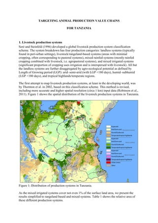
1. TARGETING ANIMAL PRODUCTION VALUE CHAINS
FOR TANZANIA
1. Livestock production systems
Seré and Steinfeld (1996) developed a global livestock production system classification
scheme. The system breakdown has four production categories: landless systems (typically
found in peri-urban settings), livestock/rangeland-based systems (areas with minimal
cropping, often corresponding to pastoral systems), mixed rainfed systems (mostly rainfed
cropping combined with livestock, i.e. agropastoral systems), and mixed irrigated systems
(significant proportion of cropping uses irrigation and is interspersed with livestock). All but
the landless systems are further disaggregated by agro-ecological potential as defined by
Length of Growing period (LGP): arid–semi-arid (with LGP <180 days), humid–subhumid
(LGP >180 days), and tropical highlands/temperate regions.
The first attempt to map livestock production systems, at least in the developing world, was
by Thornton et al. in 2002, based on this classification scheme. This method is revised,
including more accurate and higher spatial resolution (circa 1 km) input data (Robinson et al.,
2011). Figure 1 shows the spatial distribution of the livestock production systems in Tanzania.
Figure 1: Distribution of production systems in Tanzania.
As the mixed irrigated systems cover not even 1% of the surface land area, we present the
results simplified to rangeland based and mixed systems. Table 1 shows the relative area of
these different production systems.

2. Table 1: Surface area of production systems in Tanzania
2
Production system Surface area (km ) Percentage (%)
Rangeland based, (Hyper-) Arid/Semi-arid (LGA) 18,140 20
Rangeland based, Humid/Sub-humid (LGH) 7,760 9
Rangeland based, Temperate/Tropical highlands (LGT) 1,270 1
Mixed, (Hyper-) Arid/Semi-arid (MRA) 27,880 31
Mixed, Humid/Sub-humid (MRH) 14,910 17
Mixed, Temperate/Tropical highlands (MRT) 4,270 5
Urban 330 0
Other 14,010 16
Although about one third of the area in Tanzania is under grasslands supporting (agro-)
pastoral livestock production, the most common production system is mixed crop-livestock
systems, covering just over 50% of the land.
2. Socio-economic data
2.1 Human population & poverty
To show the spatial distribution of human population, we use the estimates of human
population of Global Rural-Urban Mapping Project (GRUMPv1) for the year 2000. The
population density grids measure population per square km (CIESIN, 2011). Figure 2 shows
the spatial distribution of human population densities for Tanzania.
Figure 2: Distribution of human population density in Tanzania
Table 2 shows the distribution of the population densities over the different production
systems. As expected, in the rangeland areas, the lowest population densities prevail, while
densities increase in the mixed systems. The high standard deviation in the mixed systems
highlights the large regional variation within these systems.

3. Table 2: Average population densities by production system
Production system Population density (head/km2) Standard deviation
LGA 10.1 4.9
LGH 11.1 4.8
LGT 11.3 4.2
MRA 32.7 31.8
MRH 52.0 44.1
MRT 46.3 37.5
Urban 1985.6 1072.0
Other 41.1 61.2
Poverty is defined as an economic condition in which one lacks both the money and basic
necessities, such as food, water, education, healthcare, and shelter, necessary to thrive.
Commonly measured by the average daily amount of money a person lives on, poverty is
currently set at less than US$2 (PPP) per day (also called the $ 2 poverty line) for poverty and
less than US$1.25 (PPP) per day (also called the $ 1.25 poverty line) for extreme poverty. The
most common poverty metric is head count ratio (HCR), the percentage of the population
living below the established poverty line (Wood e al, 2010).
Figure 3 shows the spatial distribution of the number of people living on less than $1.25 per
day. Figure 4 shows the spatial distribution of the number of people living on less than $2 per
day.
Figure 3: Distribution of the number of people living on less than $1.25 per day

4. Figure 4: Distribution of the number of people living on less than $2 per day
Table 3 show the total population of Tanzania by region. The table shows as well the number
of people living under 1.25$ and 2$ a day, and the percentage of poor people per region.

5. Table 3: Total population by regions, and number of people living of less than 1.25 and
2$/day
Region Total Poor people living <1.25$/day Poor people living <2$/day
population Total number % of poor Total number % of poor
(1000) (1000) people (1000) people
Arusha 1303 886 68.0 941 72.2
Dar es Salaam 2142 1,292 60.3 1,387 64.8
Dodoma 1755 1,399 79.7 1,453 82.8
Iringa 1798 1,253 69.7 1,371 76.3
Kagera 2116 1,626 76.8 1,715 81.0
Kigoma 1802 1,771 98.3 1,789 99.3
Kilimanjaro 1454 1,080 74.2 1,183 81.3
Lindi 858 819 95.5 844 98.4
Manyara 1031 775 75.2 821 79.6
Mara 1325 1,289 97.3 1,303 98.4
Mbeya 1924 1,137 59.1 1,239 64.4
Morogoro 1701 1,247 73.3 1,355 79.7
Mtwara 1133 1,079 95.3 1,128 99.6
Mwanza 2829 2,756 97.4 2,779 98.2
Pwani 931 853 91.6 898 96.5
Rukwa 1175 1,113 94.8 1,157 98.5
Ruvuma 1128 1,071 95.0 1,088 96.5
Shinyanga 2819 2,781 98.7 2,804 99.5
Singida 1100 1,092 99.3 1,094 99.4
Tabora 1738 1,704 98.0 1,719 98.9
Tanga 1629 1,280 78.6 1,373 84.3
To obtain a better idea about the distribution of the human population, Table 4 and 5 present
total population and number of poor over the different production systems.
Table 4: Total population and number of people living of less than 2$/day by production
system
Production Total Poor <2$ % poor of total % of poor persons Standard
system population poor population within farming deviation
systems
LGA 2,140,470 1,937,310 6.7 90.5 14.6
LGH 1,023,080 948,800 3.2 92.7 9.8
LGT 161,800 125,830 0.4 77.8 14.7
MRA 10,541,500 9,278,140 32.1 88.0 18.7
MRH 9,695,670 8,785,380 30.5 90.6 14.6
MRT 2,139,480 1,745,000 5.9 81.6 15.6
Urban 6,859,070 5,273,420 16.9 76.9 20.5
Other 1,439,050 1,267,200 4.3 88.1 16.9

6. Table 5: Total population and number of people living of less than 1.25$/day by production
system
Production Total Poor <2$ % poor of total % of poor persons Standard
system population poor population within farming deviation
systems
LGA 2,140,470 1,879,250 6.9 87.8 16.6
LGH 1,023,080 904,350 3.4 88.4 12.1
LGT 161,800 116,830 0.5 72.2 16.2
MRA 10,541,500 8,970,800 33.2 85.1 20.4
MRH 9,695,670 8,511,740 31.4 87.8 16.4
MRT 2,139,480 1,643,710 6.2 76.8 16.4
Urban 6,859,070 4,717,270 18.9 68.8 21.8
Other 1,439,050 1,205,680 4.5 83.8 18.0
Poverty levels are high in Tanzania. The percentages of people who are poor according to the
$1.25 a day poverty line is and $2.00 a day poverty line, is 85.6 and 89.0% respectively. As
most people live in mixed production systems, the absolute number of poor people living in
these areas is highest as well.
2.2 Market access
Travel time to market centers is used as a proxy for market accessibility and shows the likely
extent to which farming households are physically integrated with or isolated from markets. It
is important to farming households and other producers to have access to markets in order to
trade/sell their goods. The more accessible markets are to the given population the greater the
population’s ability to remain economically self-sufficient and maintain food secure (Nelson,
2008).
The travel time maps indicate the degree of accessibility to a populated place. The patterns
shown here describe the physical accessibility between places in Tanzania, whereby
accessibility is defined as the time in hours required to travel from a given single point to the
nearest market centre of 50,000 or more people. The travel time approach is estimated based
on the combination of different global spatial data layers which represent the time required to
cross each single point.

7. Figure 4: Travel time (hr) to the nearest town of 50,000 people
To obtain a better insight about the differences in travel time between production systems, the
spatial data layer of travel time was overlaid with the spatial data layer of production systems.
Table 6 shows the mean travel time for each production system.
Table 6: Mean travel time (hr) for each production system
Production system Mean travel time (hr) Standard deviation
LGA 16.2 9.1
LGH 13.3 7.4
LGT 21.3 10.5
MRA 12.7 9.1
MRH 10.8 7.2
MRT 11.7 7.9
Urban 0.8 0.7
Other 10.4 7.1
The table shows clearly that travel time in (peri-) urban areas is lowest, and that travel time
can increase quickly in the mixed systems, but with large regional variation (high standard
deviation).
To obtain a better idea about the possibilities of farmers to make use of local markets, we
combine data on population density with travel time. As a proxy for market access to local
markets, we selected all regions with a population density of more than 150 head/km2 and
those areas with a travel time of less than two hours. Figure 5 shows the spatial distribution of
access to local markets.
[In case we indeed want to use a proxy for local markets, we can play around with the cut-off
values used. In the appendix I added two figures, where used different cut-off values.]

8. Figure 5: Travel time (hr) to local markets.
2.3 Consumption
Food supply data is some of the most important data in FAOSTAT. In this report, we use
livestock consumption data to estimate national surplus – deficit areas, when it is combined
with other data sets later on (section 5).
Table 7 shows the average consumption of bovine meat, milk, pig and goat/mutton meat for
Tanzania, based on FAOSTAT for several years. Figure 6 and 7 shows the spatial distribution
of bovine meat and milk consumption, based on population density (CIESIN, 2011).
Table 7: Average consumption of livestock products in Tanzania (FAOSTAT, 2012)
Food supply quantity (kg/capita/yr)
1999 2000 2001 2002 2003 2004 2005 2006 2007
Bovine Meat 7.8 6.7 7.3 7.4 7.3 7.0 6.9 6.7 6.0
Milk, Whole 19.2 19.5 21.8 21.3 21.0 20.4 19.8 19.4 19.1
Pig meat 0.4 0.4 0.4 0.4 0.4 0.4 0.4 0.3 0.3
Mutton & Goat Meat 1.2 1.2 1.2 1.1 1.2 1.1 1.1 1.0 1.0

9. Figure 6: Average bovine meat consumption in Tanzania
Figure 7: Average bovine milk consumption in Tanzania
Table 8 shows the average meat and milk consumption over the various production systems.
The table shows clearly that most consumption takes place in urban areas, and that in the
pastoral rangelands consumption is low.

10. Table 8: Average meat and milk consumption by production systems
Production system Average milk consumption Average meat consumption
(kg/km2/year) (kg/km2/year)
LGA 203 73
LGH 225 81
LGT 222 80
MRA 663 239
MRH 1046 378
MRT 927 335
Urban 39381 14221
Other 815 294
3. Livestock
Livestock sector planning, policy development and analysis depend on reliable and accessible
information on the distribution, abundance and use of livestock. The 'Gridded Livestock of
the World' database provides standardised global, sub-national resolution maps of the major
agricultural livestock species. The map values are animal densities per square kilometre, and
are derived from official census and survey data. Livestock distribution data give an
estimation of production; they evaluate impact (both of and on livestock) by applying a
variety of rates; and they provide the denominator in prevalence and incidence estimates for
epidemiological applications, and the host distributions for transmission models (Wint &
Robinson, 2007).
Table 9 shows the number of livestock per production system. Figure 8 shows the spatial
distribution of bovine densities.
Figure 8: Average bovine densities in Tanzania

11. Table 9: Average densities of bovine, goat, pigs and sheep by production system (head/km2)
Production system Average (head/km2)
Bovine Goat Pigs Sheep
LGA 11.8 9.7 0.6 3.2
LGH 6.4 4.3 0.2 1.1
LGT 18.8 14.5 0.5 6.4
MRA 28.2 16.6 0.5 5.8
MRH 31.2 18.8 0.3 4.6
MRT 16.5 12.0 1.0 3.6
Urban 23.1 17.6 1.3 4.4
Other 8.8 9.7 0.6 2.0
Table 9 shows clearly the high densities of cattle in the mixed systems, however, it shows as
well high cattle densities in (peri-) urban systems.
The national bureau of statistics collected in the agricultural census of 2002-2003 data on the
total number of cattle by type by district (http://www.countrystat.org/tza). Based on this data
we mapped the total number of dairy cattle per district and the percentage of improved cattle.
Figure 9 and 10 show respectively the total number of improved dairy cattle and the
percentage of improved beef and dairy cattle.
Figure 9: The total number of dairy cattle

12. Figure 10: Percentage of improved cattle (%)
[We can add an appendix with data on indigenous and exotic breeds. As the tables are rather
large, I add them in Excel file until decided what data to use (http://www.nbs.go.tz/).]
4. Feeds
Herrero et al (***) estimated the consumption of feed resources (biomass use), by:
1. Estimating diets for each livestock species, in each production system
2. Estimating intake of each feed and estimating animals productivity
3. Multiplying animal productivity by the number of animals in each system (and their spatial
distribution) to get production
4. And matching this production to match national production statistics for milk, meat, etc.
Figure 11 and 12 show the spatial distribution of the biomass use of bovine feed resources for
meat and milk production in Tanzania, table 10 summarizes the feed consumption by
production system.

13. Figure 11: Bovine feed requirements for meat production in Tanzania
Figure 12: Bovine feed requirements for milk production in Tanzania

14. Table 10: Bovine feed requirements by production system
Production Average feed requirements (ton/km2/year)
system Milk production Meat production
LGA 4.1 13.0
LGH 2.7 8.8
LGT 10.1 27.9
MRA 11.0 33.0
MRH 14.9 43.4
MRT 6.3 23.0
Urban 12.9 39.5
Other 4.3 13.0
5. Production
Figure 13 and 14 shows respectively the spatial distribution of the bovine milk and meat
production for Tanzania, table 11 summarizes this production by production system.
Figure 13: Bovine milk production in Tanzania.

15. Figure 14: Bovine meat production in Tanzania.
Table 11: Bovine milk and meat production by production system
Production Average production (kg/km2/year)
system Milk Meat
LGA 666 117
LGH 1,262 35
LGT 2,794 130
MRA 1,331 273
MRH 2,555 346
MRT 1,969 151
Urban 6,418 400
Other 1,965 126
As we are interested in the surplus versus the deficit areas of milk and meat production, we
subtract the consumption data layers (figure 6 and 7) from the production layers (figure 13
and 14). Surplus areas are those areas where production exceeds the consumption; deficit
areas are those areas where local production cannot supply the consumption.
Figure 15 and 16 shows respectively the surplus - deficit areas for bovine milk and meat for
Tanzania.

16. Figure 15: Surplus - deficit areas for milk in Tanzania.
Figure 16: Surplus - deficit areas for bovine meat in Tanzania
[Several people remarked that Figure 15, doesn’t look like it is a comparison of Figures 13
and 6. I checked the data and it is the correct result of abstracting consumption data from
production data for milk. However, it was difficult to compare these figures as different
legends was used – I now changed that and the data is now presented with an identical
legend.]

17. To obtain a better idea about surplus – and deficit of cattle meat and milk in Tanzania, it is as
well needed to look at trade balances. Table 12 shows the average export of cattle, meat and
milk for the period 2000-2004 and 2005-2009.
Table 12: Export versus import of cattle in Tanzania, for between 2000-2009
item Average export Average import
2000-2004 2005-2009 2000-2004 2005-2009
Cattle meat (Tonnes) 1.4 25 30.8 32.6
Cow milk, whole, fresh (tonnes) 0.2 5.8 1164.2 2213.8
Cattle (Head) 1327 2850 72 84
The table shows clearly that Tanzania imports milk and meat in this period, but that it exports
live animals.
6 Excretion
Figure 17 shows the spatial distribution of bovine N excretion for Tanzania, table 13
summarizes this excretion by production system.
Figure 17: Bovine excretion in Tanzania.

18. Table 13: Bovine N excretion by production system
Production N excretions (kg/km2/year)
system Milk production Meat production
LGA 45 142
LGH 29 94
LGT 107 274
MRA 122 359
MRH 141 464
MRT 59 227
Urban 131 377
Other 43 128
7. Emissions
Figure 18 shows the spatial distribution of bovine emissions for Tanzania, table 14
summarizes this emissions by production system.
Figure 18: Bovine emissions in Tanzania.
Table 14: Bovine emissions by production system
Production system Emissions (ton CO2 eq/km2/year)
Milk production Meat production
LGA 3.5 163.5
LGH 2.5 17.4
LGT 9.4 47.4
MRA 8.3 363.7
MRH 11.3 26.9
MRT 5.0 44.7
Urban 11.4 14.4
Other 3.7 10.9

19. 8. Climate
Figure 19: Length of growing period (in days) for Tanzania
Table 15: Average length of growing period (days) by production system
Production system Average LGP (days)
LGA 158
LGH 202
LGT 187
MRA 154
MRH 204
MRT 192
Urban 196
Other 205
 Current climate + foreseen changes in the regions under study (CCAFS)
9. Trends
Information from the scenarios of alternative futures (Herrero et al., 2010)
 Projections of consumption of different animal products (demand)
 Feed surpluses/deficits
 Growth in animal numbers

20. Figure 20. The number of live animals per species over time

21. 10. Targeting
Figure 1: Mixed production systems (arid systems – light green; humid and temperate systems
– dark green; others - grey) versus all others
The next step is to combine Figure 1 with population density, we use a cut-off value of 25
persons/km2.
Figure 2: Areas with high population densities (dark red) versus low population densities
(pink)

22. Map A: Mixed production systems with high population densities versus others (arid systems
– light green; humid and temperate systems – dark green; others - grey)
The next step is combining Map A with market access, whereby we use a threshold of 0.5 and
5 hours.
Figure 4: Areas with good market access (dark red) versus low access (pink)

23. Map B: Mixed production systems with high population densities, and low market access
versus others (arid systems – light green; humid and temperate systems – dark green; others -
grey)
Map B gives us areas for rural production for rural consumption.
Map C: Mixed production systems with high population densities, and high market access
versus others (arid systems – light green; humid and temperate systems – dark green; others -
grey)
Map C gives us areas for rural production for urban consumption

25. 11. References
Center for International Earth Science Information Network (CIESIN), Columbia University;
International Food Policy Research Institute (IFPRI); the World Bank; and Centro
Internacional de Agricultura Tropical (CIAT). 2011. Global Rural-Urban Mapping Project,
Version 1 (GRUMPv1): Population Density Grid. Palisades, NY: Socioeconomic Data and
Applications Center (SEDAC), Columbia University.
FAOSTAT (2012)
Nelson, A. 2008. Travel time to major cities: A global map of Accessibility. Global
Environment Monitoring Unit – Joint Research Centre of the European Commission, Ispra
Italy. Available at http://gem.jrc.ec.europa.eu/
Robinson, T.P., Thornton P.K., Franceschini, G., Kruska, R.L., Chiozza, F., Notenbaert, A.,
Cecchi, G., Herrero, M., Epprecht, M., Fritz, S., You, L., Conchedda, G. & See, L. 2011.
Global livestock production systems. Rome, Food and Agriculture Organization of the United
Nations (FAO) and International Livestock Research Institute (ILRI), 152 pp.
William Wint and Timothy Robinson, 2007. Gridded livestock of the world. . Rome, Food
and Agriculture Organization of the United Nations (FAO).
Wood, S., G. Hyman, U. Deichmann, E. Barona, R. Tenorio, Z. Guo, S. Castano, O. Rivera,
E. Diaz, and J. Marin. 2010. Sub-national poverty maps for the developing world using
international poverty lines: Preliminary data release. Available from http://povertymap.info
(password protected).

26. Appendix
Alternative options for local market access indicators:
Figure A: Travel time (hr) to local markets;
travel time of less than 1 hour or with population density of 100 head/km2
Figure B: Travel time (hr) to local markets;
travel time of less than 1 hour or with population density of 150 head/km2