Slides from my talk in the tensors section.

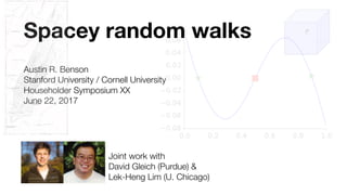
1. Spacey random walks
Austin R. Benson
Stanford University / Cornell University
Householder Symposium XX
June 22, 2017
Joint work with
David Gleich (Purdue) &
Lek-Heng Lim (U. Chicago)

2. 2
Overview of main idea
stochastic processes and (multi-)linear algebra
1
3
2
P
Px2
= x
Px = x
2
1
PRandom walk
Spacey
random walk
[Li-Ng 14; Chu-Wu 14;
Gleich-Lim-Wu 15;
Culp-Pearson-Zhang 16]
long term behavior
long term behavior

3. 1. Start with a Markov chain X0, X1, …
2. Inquire about the stationary distribution
3. Discover an eigenvector problem
3
Background Markov chains and eigenvectors
have a long-standing relationship
Px = x; ∥x∥1 = 1
Pi;j = Pr[Xt+1 = i | Xt = j]

4. 4
Higher-order means keeping more history on
the same state space.
Better model for several applications.
§ traffic flow in airport networks
[Rosvall+ 14]
§ web browsing behavior
[Chierichetti+ 12]
§ higher-order graph structure (motifs)
[Benson+ 16]
somewhat less than second order. Next, we assembled the links into networks.
All links with the same start node in the bigrams represent out-links of the start
node in the standard network (Fig. 6d). A physical node in the memory network,
which corresponds to a regular node in a standard network, has one memory node
for each in-link (Fig. 6e). A memory node represents a pair of nodes in the
trigrams. For example, the blue memory node in Fig. 6e represents passengers who
Community d
work with the
used alternati
to compare th
dynamics by
As we are int
generalization
The map e
advantage of
data. Given m
measures the
by following t
or cover of th
picking the o
The map e
dynamics, bec
walker as des
the standard
nodes to mod
movements w
random walk
nodes of the s
length must c
We achieve th
of each physi
optimal codew
depend on m
memory netw
corresponding
algorithm rem
Figure 7 il
detection. The
New York, an
order Markov
description, a
211
24,919
95,977
99,140
72.569
72.467Atlanta
Atlanta
Atlanta Atlanta
New York
New York
Chicago
Chicago
Chicago
Chicago
Chicago
San Francisco San Francisco
San Francisco
First–order Markov Second–order Markov
New York New YorkSeattle Seattle
Chicago
San Francisco San Francisco
Atlanta Atlanta
Chicago
Figure 6 | From pathway data to networks with and without memory.
(a) Itineraries weighted by passenger number. (b) Aggregated bigrams
for links between physical nodes. (c) Aggregated trigrams for links between
memory nodes. (d) Network without memory. (e) Network with
memory. Corresponding dynamics in Fig. 1a,b.
Rosvall et al., Nature Comm., 2014.
Background higher-order Markov chains are
more useful for modern data problems
Pr[Xt+1 = i | Xt = j; Xt−1 = k] = Pi;j;k
9
10
3
5
6
7
8
1
2
4
Benson et al., Science, 2016.

5. 1. Transition probability tensors represent higher-order Markov chains
2. Stationary distributions can be computed on pairs of states with a bigger
eigenvector problem. O(n2) variables.
3. Rank-1 approximation Xi,j = xixj yields a tensor z-eigenvector problem. [Li-Ng 14]
5
Background higher-order Markov chains and
tensor z-eigenvectors [Li-Ng 14]
P
j;k Pi;j;k xj xk = xi ; ∥x∥1 = 1
Px2
= x; ∥x∥1 = 1
1
3
2
P
Pi;j;k = Pr[Xt+1 = i | Xt = j; Xt−1 = k]
P
j;k Pi;j;k Xj;k = Xi;j ; ∥vec(X)∥1 = 1

6. 6
Background we are interested in z-eigenvectors for
the class of transition probability tensors
(a.k.a. stochastic hypermatrices)
P
j;k Pijk xj xk = xi ; i = 1; : : : ; n our problem
Px2
= x our problem (notation)
Ax2
= –x z-eigenvector [Qi 05]
or l2 eigenvector [Lim 05]
for order-3 tensor A

7. 7
Px2 = x has been studied as an algebraic relationship.
[Chang-Zhang 13; Li-Ng 14; Chu-Wu 14; Gleich-Lim-Wu 15; Culp-Pearson-Zhang 16]
However, we know that x (appropriately normalized) is
nonnegative and sums to 1, so it looks stochastic.
Our work gives a probabilistic interpretation of x
(and helps us study data).
Tensor z-eigenvectors:
from algebraic to stochastic

8. 8
What is the stochastic process
whose limiting distribution is the
tensor eigenvector Px2 = x?

9. 9
The spacey random walk
Pr[Xt+1 = i | Xt = j; Xt−1 = k] = Pi;j;k
1. Start with a higher-order Markov chain
2. Upon arriving at state j, we space out and forget that
we came from state k.
3. However, we still believe that we are higher-order, so we
guess state k by drawing a random state from history.

10. 10
12
4
9
7
11
4
Xt-1
Xt
Yt
Theorem [Benson-Gleich-Lim 17]
Limiting distributions of this process are tensor eigenvectors of P.
Higher-order
Markov chain
10
The spacey random walk
Pr[Xt+1 = i | Xt = j; Xt−1 = k] = Pi;j;k
Pr[Xt+1 = i | Xt = j, Yt = g] = Pi,j,g

11. 11
The spacey random walk
wt(k) = (1 +
Pt
s=1 Ind{Xs = k})/(t + n)
This is a (generalized) vertex-reinforced random walk!
[Diaconis 88; Pemantle 92, 07; Benaïm 97]
Pr[Xt+1 = i | Ft]
=
Pn
k=1 Pi;Xt ;k · wt(k)
Pr[Xt+1 = i | Ft]
= [M(wt)]i;Xt
M(wt) is a
stochastic matrix
fraction of time
spent at state k
Ft is the ff-algebra generated
by the history {X0; : : : ; Xt}

12. 12
Stationary distributions of VRRWs follow
the trajectory of ODEs
Theorem [Benaïm97] heavily paraphrased
In a discrete VRRW, the long-term behavior of the
occupancy distribution wt follows the long-term
behavior of the following dynamical system
ı maps stochastic matrix M(x)
to its stationary distribution
Key idea we study convergence of the dynamical
system for our particular map M
dx/dt = ı[M(x)] − x
M(x) =
P
k P:;:;k xk

13. dx/dt = 0
⇔ ı[M(x)] = x
⇔ M(x)x = x
⇔
P
j;k Pi;j;k xj xk = xi
⇔ Px2
= x 13
Dynamical system for VRRWs
Map for spacey random walks
Stationary point
Tensor eigenvector! (but not all are attractors)
From continuous-time dynamical systems to
tensor eigenvectors
dx/dt = ı[M(x)] − x
M(x) =
P
k P:;:;k xk

14. 14
Theory of spacey random walks
1. Nearly all 2 x 2 x 2 x … x 2 SRWs converge.
2. SRWs generalize Pólya urns processes.
3. Some convergence guarantees with Forward Euler integration
and a new algorithm for computing the eigenvector.
4. Stationary distributions can be computed in O(n) memory unlike
higher-order Markov chains.
5. If the higher-order Markov chain is really just a first-order chain,
then the SRW is identical to the first-order chain.
6. SRWs are asymptotically first-order Markovian.

15. 15
Nearly all 2 x 2 x … x 2
spacey random walks converge.

16. 16
Unfolding of P
Then
Key idea now we have a closed form, 1-dimensional ODE
p 1 q
1 p q 1
=
1 q
2 p q
1
3
2
P
Two-state dynamics
M(x) = k P:,:,kxk =
c − x1(c − a) d − x1(d − b)
1 − c + x1(c − a) 1 − d + x1(d − b)
dx/dt = ı[M(x)] − x
P(1) =
a b c d
1 − a 1 − b 1 − c 1 − d

17. 0.0 0.2 0.4 0.6 0.8 1.0
0.08
0.06
0.04
0.02
0.00
0.02
0.04
0.06
0.08
17
stable
stable
unstable
dx/dt = ı[M(x)] − x
Two-state dynamics
Theorem [Benson-Gleich-Lim 17]
The dynamics of almost every
2 x 2 x … x 2 spacey random
walk (of any order) converges
to a stable equilibrium point.
dx1
dt
x1

18. 18
Spacey random walks generalize
Pólya urn processes.

19. 19
Draw ball at random
Put ball back with another
of the same color
Two-state second-order spacey random walk
…converges!
SRWs and Pólya urn processes
P(1) =
1 1 0 0
0 0 1 1

20. 20
Draw m ball colors at
random with replacement
Put back ball of color C(b1, b2, …, bm)
b1 b2 bm
…
…converges!
SRWs and more exotic Pólya urn processes
Two-state (m+1)th-order spacey random walk
P:,:,b1,...,bm
=
I(C(b1, . . . , bm) = purple) I(C(b1, . . . , bm) = purple)
I(C(b1, . . . , bm) = green) I(C(b1, . . . , bm) = green)

21. 21
How do you compute the
tensor eigenvector Px2 = x?

22. 22
Computing the tensor eigenvectors
Our stochastic viewpoint gives a new approach.
Numerical integration of the dynamical system
for the principal eigenvector of transition prob. tensors
Current eigenpair computations are algebraic.
Power method, shifted and Newton iterations
[Li-Ng 13; Chu-Wu 14; Kolda-Mayo 14; Gleich-Lim-Yu 15]
xn+1 = Px2
n
dx
dt
=
ı[
P
k P:;:;k xk ] − x
Theorem [Benson-Gleich-Lim 17] Under some regularity conditions
of P, forward Euler method converges to a unique stable point.
Practice integrating with ode45 in Matlab always converges for any P.

23. 23
Applications of spacey random walks
1. Transportation [Benson-Gleich-Lim 17]
The SRW describes taxi cab trajectories.
2. Clustering multi-relational data [Wu-Benson-Gleich 16]
The SRW provides a new spectral clustering methodology.
3. Ranking [Gleich-Lim-Yu 15]
The SRW is gives rise to the multilinear PageRank vector, analogous
to the random surfer model for PageRank.
4. Population genetics
The SRW traces the lineage of alleles in a random mating model.
The stationary distribution is the Hardy–Weinberg equilibrium.

24. 24
Spacey random walks as a model for taxis
1,2,2,1,5,4,4,…
1,2,3,2,2,5,5,…
2,2,3,3,3,3,2,…
5,4,5,5,3,3,1,…
Model people by locations.
§ A passenger with location k is drawn at random.
§ The taxi picks up the passenger at location j.
§ The taxi drives the passenger to location i with probability Pi,j,k
Approximate location dist. by history ⟶ spacey random walk.
Urban Computing Microsoft Asia nyc.gov

25. 25
Learning from trajectories
1,2,2,1,5,4,4,…
1,2,3,2,2,5,5,…
2,2,3,3,3,3,2,…
5,4,5,5,3,3,1,…
The problem
Learn P for the spacey random walk model.
nyc.gov
The data
Sequence of taxi
trajectories.

26. 26
x(1), x(2), x(3), x(4),…
Maximum likelihood estimation problem convex
objective
linear constraints
minimize
P
Q
q=2
log
N
k=1
wk(q 1)Px(q),x(q 1),k
subject to
N
i=1
Pi,j,k = 1, 1 j, k N, 0 Pi,j,k 1, 1 i, j, k N
Learning from trajectories

27. § One year of 1000 taxi trajectories in NYC.
§ States are neighborhoods in Manhattan.
§ Learn tensor P under spacey random walk
model from training data of 800 taxis.
§ Evaluation RMSE on test data of 200 taxis.
27
First-order Markov 0.846
Second-order Markov 0.835
Spacey 0.835
NYC taxi data supports the SRW hypothesis

28. Spacey random walks
Stochastic processes for understanding eigenvectors of
transition probability tensors and analyzing higher-order data
§ The spacey random walk: a stochastic process for higher-order data.
Austin Benson, David Gleich, and Lek-Heng Lim.
SIAM Review (Research Spotlights), 2017.
https://github.com/arbenson/spacey-random-walks
§ General tensor spectral co-clustering for higher-order data.
Tao Wu, Austin Benson, and David Gleich.
In Proceedings of NIPS, 2016.
https://github.com/wutao27/GtensorSC
http://cs.cornell.edu/~arb
@austinbenson
arb@cs.cornell.edu
Thanks!
Austin Benson