Discrete Probability Distributions.

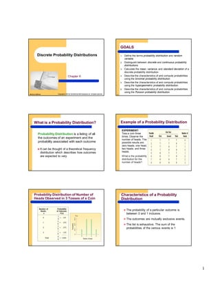
1
McGraw-Hill/Irwin Copyright © 2010 by The McGraw-Hill Companies, Inc. All rights reserved.
Discrete Probability Distributions
Chapter 6
6-2
1. Define the terms probability distribution and random
variable.
2. Distinguish between discrete and continuous probability
distributions.
3. Calculate the mean, variance, and standard deviation of a
discrete probability distribution.
4. Describe the characteristics of and compute probabilities
using the binomial probability distribution.
using the hypergeometric probability distribution.
using the Poisson probability distribution.
GOALS
6-33
What is a Probability Distribution?
Probability Distribution is a listing of all
the outcomes of an experiment and the
probability associated with each outcome
It can be thought of a theoretical frequency
distribution which describes how outcomes
are expected to vary
6-44
Example of a Probability Distribution
EXPERIMENT:
Toss a coin three
times. Observe the
number of heads. The
possible results are:
zero heads, one head,
two heads, and three
heads.
What is the probability
distribution for the
number of heads?
6-55
Probability Distribution of Number of
Heads Observed in 3 Tosses of a Coin
6-66
Characteristics of a Probability
Distribution
The probability of a particular outcome is
between 0 and 1 inclusive.
The outcomes are mutually exclusive events.
The list is exhaustive. The sum of the
probabilities of the various events is 1

2
6-7
Random Variables
RANDOM VARIABLE A quantity resulting from an experiment that, by chance, can assume different values.
EXAMPLES
1. The number of students in a class.
2. The number of children in a family.
3. The number of cars entering a carwash in a
hour.
4. Number of home mortgages approved by
Coastal Federal Bank last week.
DISCRETE RANDOM VARIABLE A random
variable that can assume only certain clearly
separated values. It is usually the result of
counting something.
EXAMPLES
1. The length of each song on the latest Tim McGraw
album.
2. The weight of each student in this class.
3. The temperature outside as you are reading this
book.
4. The amount of money earned by each of the more
than 750 players currently on Major League Baseball
team rosters.
CONTINUOUS RANDOM VARIABLE can assume an
infinite number of values within a given range. It is
usually the result of some type of measurement
6-88
The Mean of a Probability Distribution
Mean
The mean represents the central location of a
probability distribution.
The mean of a probability distribution is also
referred to as its expected value.
6-99
The Variance, and Standard Deviation of
a Discrete Probability Distribution
Variance and Standard Deviation
Measure the amount of spread in a distribution
The computational steps are:
1. Subtract the mean from each value, and square this
difference.
2. Multiply each squared difference by its probability.
3. Sum the resulting products to arrive at the variance.
The SD is the positive square root of the variance.
6-10
Mean, Variance, and Standard
Deviation of a Probability Distribution - Example
John Ragsdale sells new cars for
Pelican Ford. John usually
sells the largest number of
cars on Saturday. He has
developed the following
probability distribution for
the number of cars he
expects to sell on a
particular Saturday.
MEAN
VARIANCE
136.1290.12
 
STANDARD
DEVIATION
6-11
Expected Value Problem
Mr. Byrd has decided to print either 25, 40, 55, or 70
thousand programs. Which number of programs will minimize
the team’s expected losses?
Program Sold 25,000 40,000 55,000 70,000
Probability 0.10 0.30 0.45 0.15
Harry Byrd is trying to decide how many programs to print
for the team’s upcoming three-game series with the Oakland
A’s. Each program costs 25 cents to print and sells for $1.25.
Any programs unsold at the end of the series must be
discarded. Mr. Byrd has estimated the following probability
distribution for program sales:
6-12
Given: Per program cost = $0.25, Revenue
= $1.25 and Profit = 1.25–0.25 =1.00
X P(X)
25000
40000
55000
70000
0.10
0.30
0.45
0.15
P(X) = 1.00
Probability Distribution Table

3
6-13
Conditional Loss Table
Demand Possible Stock Options
25000 40000 55000 70000
25000
40000
55000
70000
$0
15000
30000
45000
$3750
0
15000
30000
$7500
3750
0
15000
$11250
7500
3750
0
6-14
Expected loss table for stocking 25,000 programs
Demand Condition Loss P(X) Expected Loss
25000
40000
55000
70000
$3750
0
15000
30000
0.10
0.30
0.45
0.15
$375
0
6,750
4,500
Total= $11,625
Expected loss table for stocking 40,000 programs
25000
40000
55000
70000
$0
15,000
30,000
45,000
0.10
0.30
0.45
0.15
$0
4,500
13,500
6,750
Total= $24,750
6-15
Expected loss table for stocking 55000 programs
25000
40000
55000
70000
$7500
3750
0
15000
0.10
0.30
0.45
0.15
$ 750
1,125
0
2,250
Total= $ 4,125
Expected loss table for stocking 70000 programs
25000
40000
55000
70000
$11250
7500
3750
0
0.10
0.30
0.45
0.15
1,125
2,250
1,687.5
0
Total = $5,062.5
Print55,000asthe
lossisminimum
6-1616
Binomial Probability Distribution
The Binominal Probability Distribution is
a discrete probability distribution in which
each trial or observation can assume only
one of two states.
Also called Bernoulli Process
6-1717
Binomial Probability Distribution
Characteristics
1. There are only two possible outcomes on a
particular trial of an experiment.
2. The probability of outcomes of trials remain
fixed over time.
3. Each trial is independent of any other trial.
4. The outcomes are mutually exclusive.
5. The random variable is the result of counts.
6-1818
Binomial Probability Formula

4
6-1919
Binomial Probability– Example:1
There are five flights daily from Pittsburgh via US
Airways into the Bradford, Pennsylvania, Regional
Airport. Suppose the probability that any flight
arrives late is 0.20.
(a) What is the probability that NONE of the flights
are late today?
(b) What is the probability that ONE of the flights are
late today?
3277.0)3277)(.1)(1(
)20.0-1()20.0(
)-1()()0(
0-50
05
-



C
CP xnx
xn 
4096.0=)4096)(.20.0)(5(=
)20.0–1()20.0(C=
)π–1()π(C=)1(P
1–51
15
x–nx
xn
6-2020
For the example regarding the
number of late flights, recall
that  =.20 and n = 5.
What is the average number
of late flights?
What is the variance of the
number of late flights?
Binomial Distribution – Mean and
Variance: Example
6-2121
Binomial Distribution – Mean and
Variance: Another Solution
6-22
Binomial Distribution - Example
EXAMPLE
Five percent of the worm gears
produced by an automatic, high-
speed Carter-Bell milling machine
are defective.
What is the probability that out of six
gears selected at random none will
be defective? Exactly one? Exactly
two? Exactly three? Exactly four?
Exactly five? Exactly six out of six?
Binomial – Shapes for Varying  (n constant)
Binomial – Shapes for Varying n ( constant)
6-23
Harry Ohme is in charge of the electronics section of a
large department store. He has noticed that the probability
that a customer who is just browsing will buy something is
0.3. Suppose that 15 customers browse in the electronics
section each hour.
(a) What is the probability that at least one browsing
customer will buy something during a specified hour?
(b) What is the probability that at least four browsing
customers will buy something during a specified hour?
(c) What is the probability that no browsing customers will
buy anything during a specified hour?
(d) What is the probability that no more than four browsing
customers will buy something during a specified hour?
Binomial Probability (Levin and Rubin)
6-24
9953.0=)30.0–1()30.0(C-1=
)π–1()π(C=)1x(P)a(
0–510
015
x–nx
xn
≥
7032.0=
]1700.0+0916.0+0.0305+[0.0047–1
])30.–1()30(.C+)30.–1()30(.C+
)30.–1()30(.C+)30.–1()30(.C-[1=
P(3)]+P(2)+P(1)+[P(0)-1=
)π–1()π(C=)4x(P)b(
3–513
315
2–512
215
1–511
115
0–510
015
x–nx
xn≥

5
6-25
0047.0=)30.0–1()30.0(C=
)π–1()π(C=)0=x(P)c(
0–510
015
x–nx
xn
5154.0=
]2186.0+1700.0+0916.0+0.0305+[0.0047=
])30.–1()30(.C+
)30.–1()30(.C+)30.–1()30(.C+
)30.–1()30(.C+)30.–1()30(.C[=
P(4)]+P(3)+P(2)+P(1)+[P(0)=)4x(P)d(
4–514
415
3–513
315
2–512
215
1–511
115
0–510
015
≤
6-26
The latest nationwide political poll indicates that for
Americans who are randomly selected, the probability
that they are conservative is 0.55, the probability that
they are liberal is 0.30, and the probability that they are
middle-of-the-road is 0.15. Assuming that these
probabilities are accurate, answer the following the
questions pertaining to a randomly chosen group of 10
Americans.
(a) What is the probability that 4 are liberal ?
(b) What is the probability that none are conservative ?
(c) What is the probability that 2 are middle-of-the-road ?
(d) What is the probability that 8 are liberal ?
6-27
0003.0=)3.–1()3(.C=)π–1()π(C=)4(P)a( 4–014
410
x–nx
xn
2001.0=)55.–1()55(.C=)π–1()π(C=)10(P)b( 0–014
010
x–nx
xn
2759.0=)51.–1()15(.C=)π–1()π(C=)2(P)c( 2–014
210
x–nx
xn
00160.0=
00001.0+00014.0+00145.0=
)3.–1()3(.C
+)3.–1()3(.C+)3.–1()3(.C=
)10(P+)9(P+)8(P=)π–1()π(C=)8≥x(P)d(
01–0110
10
9–019
9
8–018
810
x–nx
xn
6-28
Problems Related to Meeting Conditions
of Binomial Distribution
In real life problems, the probability of
success or failure does not remain fixed
all the time
The trials may not be statistically
independent of each other
6-2929
Binomial – Shapes for Varying 
(n constant)
6-3030
Binomial – Shapes for Varying n
( constant)

6
6-3131
Cumulative Binomial Probability
Distribution
A study in June 2003 by the Illinois Department of
Transportation concluded that 76.2% of front seat
occupants used seat belts. A sample of 12 vehicles is
selected. What is the probability the front seat
occupants in at least 7 of the 12 vehicles are wearing
seat belts?
6-3232
Poisson Probability Distribution
The Poisson probability distribution
describes the number of times some event
occurs during a specified interval. The interval
may be time, distance, area, or volume.
Assumptions of the Poisson Distribution
(1) The random variable is the number of times some
event occurs during a defined interval
(2) The probability is proportional to the length of the
interval.
(3) The intervals don’t overlap and are independent.
6-3333
Poisson Probability Distribution
The Poisson distribution can be described
mathematically using the formula:
6-3434
Mean and Variance of Poisson
Probability Distribution
The mean number of successes  can
be determined in binomial situations by
n, where n is the number of trials and
 the probability of a success.
The variance of the Poisson distribution
is also equal to n .
6-3535
Assume baggage is rarely lost by Northwest
Airlines. Suppose a random sample of 1,000
flights shows a total of 300 bags were lost. Thus,
the arithmetic mean number of lost bags per flight
is 0.3 (300/1,000). If the number of lost bags per
flight follows a Poisson distribution with u = 0.3,
find the probability of not losing any bags.
Poisson Probability Distribution–
Example:1
6-3636
Poisson Probability Distribution- Table
Assume baggage is rarely lost by Northwest Airlines. Suppose a
random sample of 1,000 flights shows a total of 300 bags were lost.
Thus, the arithmetic mean number of lost bags per flight is 0.3
(300/1,000). If the number of lost bags per flight follows a Poisson
distribution with mean = 0.3, find the probability of not losing any bags.

7
6-37
More About the Poisson Probability
Distribution
•The Poisson probability distribution is always positively skewed and the
random variable has no specific upper limit.
•The Poisson distribution for the lost bags illustration, where µ=0.3, is highly
skewed.
•As µ becomes larger, the Poisson distribution becomes more symmetrical.
6-38
1465.=
!2
e4
=
!x
eµ
=)x(P
4–2u–x
The Lab Aid specializes in
caring for minor injuries,
colds, and flu. For the
evening hours of 6-10 PM
the mean number of arrivals
is 4.0 per hour. What is the
probability of 2 arrivals in an
hour?
Example:2
6-39
The US Bureau of Printing and Engraving (BPE)
is responsible for printing this country’s paper
money. The BPE has an impressively small
frequency of printing errors; only 0.5 percent of
all bills are too flawed for circulation. What is the
probability that out of a batch of 1,000 bills
(a) None are too flawed for circulation?
(b) Ten are flawed for circulation?
(c) Fifteen are flawed for circulation?
Example:3
6-40
Example:3
01813.0=
!10
e×)5(
=)10(P
5–10
00016.0=
!15
e×)5(
=)15(P
5–15
Given us: n = 1000, π = 0.005
Thus: µ =nπ = (1000)(0.005) = 5
00674.0=
!0
e5
=
!x
eµ
=)0(P
5–0u–x
6-41
Concert Pianist Donna Prima has become quite
upset at the number of coughs occurring in the
audience just before she begins to play. On her
latest tour, Donna estimates that on average eight
coughs occur just before the start of her
performance. Ms. Prima has sworn to her
conductor that if she hears more than five coughs
at tonight’s performance, she will refuse to play.
What is the probability that she will not play
tonight?
Example:4
6-42
Example:4
8088.0=0.1912–1=
0.0916]+0.0573+0.0286+
0.0107+0.0027+[0.0003–1=
]
!5
e×)8(
+
!4
e×)8(
+
!3
e×)8(
+
!2
e×)8(
+
!1
e×)8(
+
!0
e×)8(
[–1=
8–58–48–3
8–28–18–0
Given us: µ = 8
)]5(P+)4(P+)3(P+)2(P+)1(P+)0(P[–1

8
6-43
Poisson Distribution as an
Approximation of Binomial Distribution
The Poisson Distribution is a good
approximation of the Binomial Distribution
when n ≥ 20 and π ≤ 0.05.
6-44
A hospital has 20 kidney dialysis machines and that the
chance of any of them malfunctioning during any day is
0.02. What is the probability that exactly three
machines will be out of service on the dame day?
!x
e×)πn(
=)x(P
)πn(–x
007.0=
6
e×)4.0(
=
!3
e×)02.0×20(
=)3(P
)4.0(–3
)02.0×20(–3
006.0=
).020-1()02.0(C=)3(P
)π-1()π(C=)x(P
3-023
320
x-nx
xn
Approximation of Binomial Distribution:
An Example
Binomial DistributionPoisson Distribution
6-45
Hypergeometric Probability Distribution
1. An outcome on each trial of an experiment is
classified into one of two mutually exclusive
categories—a success or a failure.
2. The probability of success and failure changes from
trial to trial.
3. The trials are not independent, meaning that the
outcome of one trial affects the outcome of any
other trial.
Note: Use hypergeometric distribution if experiment is
binomial, but sampling is without replacement from a
finite population where n/N is more than 0.05
Formula:
EXAMPLE
PlayTime Toys, Inc., employs 50 people in the
Assembly Department. Forty of the employees
belong to a union and ten do not. Five employees
are selected at random to form a committee to
meet with management regarding shift starting
times.
What is the probability that four of the five selected
for the committee belong to a union?
Here’s what’s given:
N = 50 (number of employees)
S = 40 (number of union employees)
x = 4 (number of union employees selected)
n = 5 (number of employees selected)
6-4646
End of Chapter 6

Discrete Probability Distributions.

Recomendados

Recomendados

Más contenido relacionado

La actualidad más candente

La actualidad más candente (20)

Destacado

Destacado (16)

Similar a Discrete Probability Distributions.

Similar a Discrete Probability Distributions. (20)

Más de ConflagratioNal Jahid

Más de ConflagratioNal Jahid (9)

Último

Último (20)

Discrete Probability Distributions.