Plc 2

Learning System for Automation and Technology
093311
Programmable logic
controllers
Basic level TP301 – Textbook
TP
IN
PT
Q
TP_1Y1
T#5s ET
S1 1B1 1Y1
&S1 TP
IN
PT
Q 1Y1
TP_1Y1
1B1
T#5s
ET
1A1
4 2
5 3
1
1V1
1Y1

TP301 • Festo Didactic
B-II
Authorised applications and liability
The Learning System for Automation and Technology has been devel-
oped and prepared exclusively for training in the field of automation. The
training organization and/or trainee shall ensure that the safety precau-
tions described in the accompanying Technical documentation are fully
observed.
Festo Didactic hereby excludes any liability for injury to trainees, to the
training organization and/or to third parties occurring as a result of the
use or application of the station outside of a pure training situation, un-
less caused by premeditation or gross negligence on the part of Festo
Didactic.
Order No.: 093311
Description: SPS LB GS
Designation: D.LB-TP301–1-GB
Edition: 08/2002
Layout: 28.08.2002, OCKER Ingenieurbüro
Graphics: D. Schwarzenberger, OCKER Ingenieurbüro
Authors: R. Bliesener, F.Ebel, C.Löffler, B. Plagemann,
H.Regber, E.v.Terzi, A. Winter
© Copyright by Festo Didactic GmbH & Co., D-73770 Denkendorf 2002
The copying, distribution and utilization of this document as well as the
communication of its contents to others without expressed authorization
is prohibited. Offenders will be held liable for the payment of damages.
All rights reserved, in particular the right to carry out patent, utility model
or ornamental design registrations.
Parts of this training documentation may be duplicated, solely for training
purposes, by persons authorised in this sense.

B-III
Preface
The programmable logic controller represents a key factor in industrial
automation. Its use permits flexible adaptation to varying processes as
well as rapid fault finding and error elimination.
This textbook explains the design of a programmable logic controller and
its interaction with peripherals.
One of the main focal points of the textbook deals with the new interna-
tional standard for PLC programming, the EN 61131-3 (IEC-61131-3).
This standard takes into account expansions and developments, for
which no standardised language elements existed hitherto.
The aim of this new standard is to standardise the design, functionality
and the programming of a PLC in such a way as to enable the user to
easily operate with different systems.
In the interest of continual further improvement, all readers of this book
are invited to make contributions by way suggestions, ideas and con-
structive criticism.
August 2002 The authors

B-V
Table of Contents
Chapter 1 Automating with a PLC B-1
1.1 Introduction B-1
1.2 Areas of application of a PLC B-2
1.3 Basic design of a PLC B-5
1.4 The new PLC standard EN 61131 (IEC 61131) B-8
Chapter 2 Fundamentals B-11
2.1 The decimal number system B-11
2.2 The binary number system B-11
2.3 The BCD code B-13
2.4 The hexadecimal number system B-13
2.5 Signed binary numbers B-14
2.6 Real numbers B-14
2.7 Generation of binary and digital signals B-15
Chapter 3 Boolean operations B-19
3.1 Basic logic functions B-19
3.2 Further logic operations B-23
3.3 Establishing switching functions B-25
3.4 Simplification of logic functions B-28
3.5 Karnaugh-Veitch diagram B-30

B-VI
Chapter 4 Design and mode of operation of a PLC B-33
4.1 Structure of a PLC B-33
4.2 Central control unit of a PLC B-35
4.3 Function mode of a PLC B-37
4.4 Application program memory B-39
4.5 Input module B-41
4.6 Output module B-43
4.7 Programming device/Personal computer B-45
Chapter 5 Programming of a PLC B-47
5.1 Systematic solution finding B-47
5.2 EN 61131-3 (IEC 61131-3) structuring resources B-50
5.3 Programming languages B-54
Chapter 6 Common elements of programming languages B-57
6.1 Resources of a PLC B-57
6.2 Variables and data types B-60
6.3 Program B-70
Chapter 7 Function block diagram B-85
7.1 Elements of function block diagram B-85
7.2 Evaluation of networks B-85
7.3 Loop structures B-87
Chapter 8 Ladder diagram B-89
8.1 Elements of ladder diagram B-89
8.2 Functions and function blocks B-92
8.3 Evaluation of current rungs B-93

B-VII
Chapter 9 Instruction list B-95
9.1 Instructions B-95
9.2 Operators B-96
9.3 Functions and function blocks B-97
Chapter 10 Structured text B-99
10.1 Expressions B-99
10.2 Statements B-101
10.3 Selection statements B-103
10.4 Iteration statements B-106
Chapter 11 Sequential function chart B-111
11.2 Elements of sequential function chart B-111
11.3 Transitions B-120
11.4 Steps B-123
11.5 Example B-135
Chapter 12 Logic control systems B-139
12.1 What is a logic control system B-139
12.2 Logic control systems without latching properties B-139
12.3 Logic control systems with memory function B-145
12.4 Edge evaluation B-148
Chapter 13 Timers B-153
13.2 Pulse timer B-154
13.3 Switch-on signal delay B-156
13.4 Switch-off signal delay B-158

B-VIII
Chapter 14 Counter B-161
14.1 Counter functions B-161
14.2 Incremental counter B-161
14.3 Decremental counter B-165
14.4 Incremental/decremental counter B-167
Chapter 15 Sequence control systems B-169
15.1 What is a sequence control system B-169
15.2 Function chart to IEC 60848 B-169
Chapter 16 Commissioning and
operational safety of a PLC B-175
16.1 Commissioning B-175
16.2 Operational safety of a PLC B-177
Chapter 17 Communication B-183
17.1 The need for communication B-183
17.2 Data transmission B-183
17.3 Interfaces B-184
17.4 Communication in the field area B-185
Appendix
A Bibliography of illustrations B-187
B Bibliography of literature B-189
C Guidelines and standards B-191
D Glossary B-193
E Index B-199

B-1
Chapter 1
The PLC in automation technology
1.1 Introduction
The first Programmable Logic Controller (PLC) was developed by a
group of engineers at General Motors in 1968, when the company were
looking for an alternative to replace complex relay control systems.
The new control system had to meet the following requirements:
Simple programming
Program changes without system intervention
(no internal rewiring)
Smaller, cheaper and more reliable than corresponding relay control
systems
Simple, low cost maintenance
Subsequent development resulted in a system, which enabled the sim-
ple connection of binary signals. The requirements as to how these sig-
nals were to be connected were specified in the control program. With
the new systems it became possible for the first time to plot signals on a
screen and to file these in electronic memories.
Since then, three decades have passed, during which the enormous
progress made in the development of microelectronics did not stop short
of programmable logic controllers. For instance, even if program optimi-
sation and thus a reduction of required memory capacity initially still rep-
resented an important key task for the programmer, nowadays this is
hardly of any significance.
Moreover, the range of functions has grown considerably. 15 years ago,
process visualisation, analogue processing or even the use of a PLC as
a controller, were considered as Utopian. Nowadays, the support of
these functions forms an integral part of many PLCs.
The following pages in this introductory chapter outline the basic design
of a PLC together with the currently most important tasks and applica-
tions.

B-2
Chapter 1
1.2 Areas of application of a PLC
Every system or machine has a controller. Depending on the type of
technology used, controllers can be divided into pneumatic, hydraulic,
electrical and electronic controllers. Frequently, a combination of differ-
ent technologies is used. Furthermore, differentiation is made between
hard-wired programmable (e.g. wiring of electro-mechanical or electronic
components) and programmable logic controllers. The first is used pri-
marily in cases, where any reprogramming by the user is out of the
question and the job size warrants the development of a special control-
ler. Typical applications for such controllers can be found in automatic
washing machines, video cameras, and cars.
However, if the job size does not warrant the development of a special
controller or if the user is to have the facility of making simple or inde-
pendent program changes, or of setting timers and counters, then the
use of a universal controller, where the program is written to an elec-
tronic memory, is the preferred option. The PLC represents such a uni-
versal controller. It can be used for different applications and, via the
program installed in its memory, provides the user with a simple means
of changing, extending and optimising control processes.

B-3
Chapter 1
The original task of a PLC involved the interconnection of input signals
according to a specified program and, if "true", to switch the correspond-
ing output. Boolean algebra forms the mathematical basis for this opera-
tion, which recognises precisely two defined statuses of one variable: "0"
and "1" (see also chapter 3). Accordingly, an output can only assume
these two statuses. For instance, a connected motor could therefore be
either switched on or off, i.e. controlled.
This function has coined the name PLC: Programmable logic control-
ler, i.e. the input/output behaviour is similar to that of an electro-
magnetic relay or pneumatic switching valve controller; the program is
stored in an electronic memory.
However, the tasks of a PLC have rapidly multiplied: Timer and counter
functions, memory setting and resetting, mathematical computing opera-
tions all represent functions, which can be executed by practically any of
today’s PLCs.
Fig. B1.1:
Example of a
PLC application

B-4
Chapter 1
The demands to be met by PLC’s continued to grow in line with their
rapidly spreading usage and the development in automation technology.
Visualisation, i.e. the representation of machine statuses such as the
control program being executed, via display or monitor. Also controlling,
i.e. the facility to intervene in control processes or, alternatively, to make
such intervention by unauthorised persons impossible. Very soon, it also
became necessary to interconnect and harmonise individual systems
controlled via PLC by means of automation technology. Hence a master
computer facilitates the means to issue higher-level commands for pro-
gram processing to several PLC systems
The networking of several PLCs as well as that of a PLC and master
computer is effected via special communication interfaces. To this effect,
many of the more recent PLCs are compatible with open, standardised
bus systems, such as Profibus to EN 50170. Thanks to the enormously
increased performance capacity of advanced PLCs, these can even di-
rectly assume the function of a master computer.
At the end of the seventies, binary inputs and outputs were finally ex-
panded with the addition of analogue inputs and outputs, since many of
today’s technical applications require analogue processing (force meas-
urement, speed setting, servo-pneumatic positioning systems). At the
same time, the acquisition or output of analogue signals permits an ac-
tual/setpoint value comparison and as a result the realisation of auto-
matic control engineering functions, a task, which widely exceeds the
scope suggested by the name (programmable logic controller).
The PLCs currently on offer in the market place have been adapted to
customer requirements to such an extent that it has become possible to
purchase an eminently suitable PLC for virtually any application. As
such, miniature PLCs are now available with a minimum number of in-
puts/outputs starting from just a few hundred Pounds. Also available are
larger PLCs with 28 or 256 inputs/outputs.
Many PLCs can be expanded by means of additional input/output, ana-
logue, positioning and communication modules. Special PLCs are avail-
able for safety technology, shipping or mining tasks. Yet further PLCs
are able to process several programs simultaneously – (multitasking).
Finally, PLCs are coupled with other automation components, thus cre-
ating considerably wider areas of application.

B-5
Chapter 1
1.3 Basic design of a PLC
The term ’programmable logic controller’ is defined as follows by
EN 61131-1 (IEC 61131-1):
“ A digitally operating electronic system, designed for use in an industrial
environment, which uses a programmable memory for the internal stor-
age of user-oriented instructions for implementing specific functions
such as logic, sequencing, timing, counting and arithmetic, to control,
through digital or analogue inputs and outputs, various types of ma-
chines or processes.
Both the PC and its associated peripherals are designed so that they
can be easily integrated into an industrial control system and easily used
in all their intended functions."
A programmable logic controller is therefore nothing more than a com-
puter, tailored specifically for certain control tasks.
Fig. B1.2:
Example of a PLC:
Festo IPC PS1 Professional

B-6
Chapter 1
Fig. B1.3 illustrates the system components of a PLC.
PLC-program
Central control unitInput module Output module
ActuatorsSensors
The function of an input module is to convert incoming signals into sig-
nals, which can be processed by the PLC, and to pass these to the cen-
tral control unit. The reverse task is performed by an output module. This
converts the PLC signal into signals suitable for the actuators.
The actual processing of the signals is effected in the central control unit
in accordance with the program stored in the memory.
The program of a PLC can be created in various ways: via assembler-
type commands in ’statement list’, in higher-level, problem-oriented lan-
guages such as structured text or in the form of a flow chart such as
represented by a sequential function chart. In Europe, the use of func-
tion block diagrams based on function charts with graphic symbols for
logic gates is widely used. In America, the ’ladder diagram’ is the pre-
ferred language by users.
Depending on how the central control unit is connected to the input and
output modules, differentiation can be made between compact PLCs
(input module, central control unit and output module in one housing) or
modular PLCs.
Fig. B1.3:
System components
of a PLC

B-7
Chapter 1
Fig. B1.4 shows the FX0 controller by Mitsubishi and the IPC FEC Stan-
dard controller by Festo as an Example
Modular PLCs may be configured individually. The modules required for
the practical application – apart from digital input/output modules, which
can, for instance, include analogue, positioning and communication
modules – are inserted in a rack, where individual modules are linked via
a bus system. This type of design is also known as series technology.
Two examples of modular PLCs are shown in figs. B1.2 and B1.4. These
represent the modular system IPC PS1 Professional by Festo and the
new S7-300 series by Siemens.
Fig. B1.4:
Compact-PLC
(Mitsubishi FX0,
Festo IPC FEC Standard),
modular PLC
(Siemens S7-300)

B-8
Chapter 1
A wide range of variants exists, particularly in the case of more recent
PLCs. These include both modular as well as compact characteristics
and important features such as spacing saving, flexibility and scope for
expansion.
The card format PLC is a special type of modular PLC, developed during
the last few years. With this type, individual or a number of printed circuit
board modules are in a standardised housing.
The hardware design for a programmable logic controller is such that it
is able to withstand typical industrial environments as regard signal lev-
els, heat, humidity, and fluctuations in current supply and mechanical
impact.
1.4 The new PLC standard EN 61131 (IEC 61131)
Previously valid PLC standards focussing mainly on PLC programming
were generally geared to current state of the art technology in Europe at
the end of the seventies. This took into account non-networked PLC
systems, which primarily execute logic operations on binary signals.
Previously, no equivalent, standardised language elements existed for
the PLC developments and system expansions made in the eighties,
such as processing of analogue signals, interconnection of intelligent
modules, networked PLC systems etc. Consequently, PLC systems by
different manufacturers required entirely different programming.
Since 1992, an international standard now exists for programmable logic
controllers and associated peripheral devices (programming and diag-
nostic tools, testing equipment, man-to-machine interfaces etc.). In this
context, a device configured by the user and consisting of the above
components is known as a PLC system.

B-9
Chapter 1
The new EN 61131 (IEC 61131) standard consists of five parts:
Part 1: General information
Part 2: Equipment requirements and tests
Part 3: Programming languages
Part 4: User guidelines (in preparation with IEC)
Part 5: Messaging service specification (in preparation with IEC)
Parts 1 to 3 of this standard were adopted unamended as European
Standard EN 61 131, Parts 1 to 3.
The purpose of the new standard was to define and standardise the de-
sign and functionality of a PLC and the languages required for pro-
gramming to the extent where users were able to operate using different
PLC systems without any particular difficulties.
The next chapters will be dealing with this standard in greater detail.
However, for the moment the following information should suffice:
The new standard takes into account as many aspects as possible
regarding the design, application and use of PLC systems.
The extensive specifications serve to define open, standardised PLC
systems.
Manufacturers must conform to the specifications of this standard
both with regard to purely technical requirements for the PLC as well
as the programming of controllers.
Any variations must be fully documented for the user.
After initial reservations, a large group of interested people (PLCopen)
has been formed to support this standard. A large number of major PLC
suppliers are members of the association, i.e. ABB, GE Fanuc, Mitsubi-
shi Electric, Moeller, OMRON, Schneider Electric, Siemens.
A large number of the members of the association offer control and pro-
gramming systems conforming to EN 61131 (IEC 61131).
In the future, languages in accordance with IEC 61131 will not only
dominate PLC programming, but rather industrial automation in its en-
tirety.

B-10
Chapter 1

B-11
Chapter 2
Fundamentals
2.1 The decimal number system
Characteristic of the decimal number system used in general is the lin-
ear array of digits and their significant placing. The number 4344, for
instance, can be represented as follows:
4344 = 4 x 1000 + 3 x 100 + 4 x 10 + 4 x 1
Number 4 on the far left is of differing significance to that of number 4 on
the far right.
The basis of the decimal number system is the availability of 10 different
digits (decimal: originating from the Latin ’decem’ = 10 ). These 10 dif-
ferent digits permit counting from 0 to 9. If counting is to exceed the
number 9, this constitutes a carry over to the next place digit. The sig-
nificance of this place is 10, and the next carry over takes place when 99
is reached.
The number 71.718.711 is to be used as an example:
10
7
10
6
10
5
10
4
10
3
10
2
10
1
10
0
7 1 7 1 8 7 1 1
As can be seen from the above, the significance of the "7" on the far left
is 70.000.000 = 70 million, whereas the significance of the "7" in the third
place from the right is 700.
The digit on the far right is referred to as the least significant digit, and
the digit on the far left as the most significant digit.
Any number system can be configured on the basis of this example, the
fundamental structure can be applied to number systems of any number
of digits. Consequently, any computing operations and computing meth-
ods which use the decimal number system can be applied with other
number systems.
2.2 The binary number system
We are indebted to Leibnitz, who applied the structures of the decimal
number system to two-digit calculation. As long ago as 1679, this cre-
ated the premises essential for the development of the computer, since
electrical voltage or electrical current only permits a calculation using
just two values: e.g. "current on", "current off". These two values are
represented in the form of digits: "1" and "0".
Example

B-12
Chapter 2
If one were to be limited to exactly 2 digits per place of a number, then a
number system would be configured as follows:
27
= 128 26
= 64 25
= 32 24
= 16 23
= 8 22
= 4 21
= 2 20
= 1
1 0 1 1 0 0 0 1
The principle is exactly the same as that of the method used to create a
decimal number. However, only two digits are available, which is why
the significant place is not calculated to the base 10x, but to the base 2x.
Hence the lowest significant number on the far right is0
= 1, and of the
next place 21
= 2 etc. Because of the exclusive use of two digits, this
number system is known as the binary or also the dual number system.
Up to a maximum of
28
– 1 = 256 – 1 = 255
can be calculated with eight places, which would be the
number 1111 11112.
The individual places of the binary number system can adopt one of the
two digits 0 or 1. This smallest possible unit of the binary system is
termed 1 bit.
In the above example, a number consisting of 8 bits, i.e. one byte, has
been configured (in a computer using 8 electrical signals representing
either "voltage available" or "voltage not available" or "current on" or
"current off".) The number considered, 1011 00012, assumes the deci-
mal value 17710.
1 x 27
0 x 26
1 x 25
1 x 24
0 x 23
0 x 22
0 x 21
1 x 20
= 128 + 32 + 16 1
= 177
Example
Example

B-13
Chapter 2
2.3 The BCD code
For people used to dealing with the decimal system, binary numbers are
difficult to read. For this reason, a more easily readable numeral repre-
sentation was introduced; i.e. the binary coded decimal notation, the so-
called BCD code (binary coded decimal). With this BCD code, each indi-
vidual digit of the decimal number system is represented by a corre-
sponding binary number:
010 0000BCD
110 0001BCD
210 0010BCD
310 0011BCD
410 0100BCD
510 0101BCD
610 0110BCD
710 0111BCD
810 1000BCD
910 1001BCD
4 digits in binary notation are therefore required for the 10 digits in the
decimal system. The discarded place (in binary notation, the numbers 0
to 15 may be represented with 4 digits) is accepted for the sake of clar-
ity.
The decimal number 7133 is thus represented as follows in the BCD
code:
0111 0001 0011 0011BCD
16 bits are therefore required to represent a four digit decimal number in
the BCD code. BCD coded numbers are often used for seven segment
displays and coding switches.
2.4 The hexadecimal number system
The use of binary numbers is often difficult for the uninitiated and the
use of the BCD code takes up a lot of space. This is why the octal and
the hexadecimal system were developed. Three digits are always com-
bined in the case of the octal number system. This permits counting from
0 to 7, i.e. counting in "eights".
Table B2.1:
Representation of decimal
numbers in BCD code

B-14
Chapter 2
Alternatively, 4 bits are combined with the hexadecimal number system.
4 bits permit the representation of the numbers 0 to 15, i.e. counting in
"sixteens". The digits 0 to 9 are used to represent these numbers in dig-
its, followed by the letters A, B, C, D, E and F where A = 10, B = 11, C =
12, D = 13, E = 14 and F = 15. The significant place of the individual
digits is to the base 16.
163
= 4096 162
= 256 161
= 16 160
= 1
8 7 B C
The number 87BC16 given as an example therefore reads as follows:
8 x 163
+ 7 x 162
+ 11 x 161
+ 12 x 160
= 34 74810
2.5 Signed binary numbers
Up to now, we have dealt solely with whole positive numbers, not taking
into account negative numbers. To enable working with these negative
numbers, it was decided that the most significant bit on the far left of a
binary number is to be used to represent the preceding sign: "0" thus
corresponds to "+" and "1" corresponds to "–".
Hence 1111 11112 = -12710 and 0111 11112 = +12710
Since the most significant bit has been used, one bit less is available for
the representation of a signed number. In the field of data processing,
the use of so-called compliment representation for the expression of
negative numbers has proven useful. The following range of values is
obtained for the representation of a 16 digit binary number:
Integer Range of values
unsigned 0 to 65535
signed -32768 to +32767
2.6 Real numbers
Although it is now possible for whole positive and whole signed numbers
to be represented with 0 or 1, there is still the need for points or real
numbers.
In order to represent a real number in computer binary notation, the
number is split into two groups, a power of ten and a multiplication fac-
tor. This is also known as the scientific representation of digits.
Example
Example

B-15
Chapter 2
The number 27,3341 is thus converted into 273 341 x 10-4. Two whole-
signed numbers are therefore required for a real number to be repre-
sented in a computer.
2.7 Generation of binary and digital signals
As has already become clearly apparent in the previous section, all
computers and as such all PLCs operate using binary or digital signals.
By binary signal, we understand a signal, which recognises only two
defined values.
1
t
0
These values are termed "0" or "1", the terms "low" and "high" are also
used. The signals can be very easily realised with contacting compo-
nents. An actuated normally open contact corresponds to a logic 1-
signal and an unactuated one to a logic 0-signal. When working with
contactless components, this can give rise to certain tolerance bands.
For this reason, certain voltage ranges have been defined as logic 0 or
logic 1 ranges.
V
0
5
11
30
t-3
1 - range
0 - range
Fig. B2.1:
Binary signal
Fig. B2.2:
Voltage ranges

B-16
Chapter 2
EN 61131-2 (IEC 61131-2) defines a value range of -3 V to 5 V as logic
0-signal, and 11 V to 30 V as logic 1-signal (for contactless sensors).
This is binding for PLCs, whose device technology is to conform to EN
61131-2 (IEC 61131-2). In current practice, however, other voltage
ranges can often be found for logic 0- and 1-signal. Widely used are: -30
V to +5 V as logic 0, 13 V to 30 V as logic 1.
Unlike binary signals, digital signals can assume any value. These are
also referred to as value stages. A digital signal is thus defined by any
number of value stages. The change between these is non-sequential.
The following illustration shows three possible methods of converting an
analogue signal into a digital signal.
t
0
V
1
2
3
4
5
6 Digital Signal
on 0,5V basis
Digital
Signal on
3V basis
Analogues Signal
Digital Signal
on 1V basis
Digital signals may be formed from analogue signals. This method is for
instance used for analogue processing via PLC. Accordingly, the ana-
logue input signal within a range of 0 to 10 V is reduced into a series of
step values. Depending on the quality of the PLC and the possible step
height set, the digital signal would thus be able to operate in steps of
value of 0.1 V, 0.01 V or 0.001 V. Naturally, the smallest range is se-
lected in this instance in order for the analogue signal to be reproduced
as accurately as possible.
Fig. B2.3:
Conversion of an analogue
signal into a digital signal

B-17
Chapter 2
One simple example of an analogue signal is pressure, which is meas-
ured and displayed by a pressure gauge. The pressure signal may as-
sume any intermediate value between its minimum and maximum
values. Unlike the digital signal, it changes continually. In the case of the
processing of analogue values via a PLC, as described, analogue volt-
age signals are evaluated and converted.
On the other hand, digital signals can be formed by adding together a
certain number of binary signals. In this way, again as described in the
above paragraph, it is also possible to generate a digital signal with 256
step values.
Bit No. 7 6 5 4 3 2 1 0 Digital value
Example 1 1 0 1 1 1 0 1 1 187
Example 2 0 0 1 1 0 0 1 1 51
Example 3 0 0 0 0 0 0 0 0 0
This process is for instance used to implement timer and counter func-
tions.
Example

B-18
Chapter 2

B-19
Chapter 3
Boolean operations
3.1. Basic logic functions
As described in the previous chapter, any computer and equally any
PLC operates using the number system to the base 2. This also applies
to the octal (23
) and the hexadecimal systems (24
). The individual vari-
able can therefore assume only two values, "0" or "1". Special algo-
rithms have been introduced to be able to link these variables – the so-
called boolean algebra. This can be clearly represented by means of
electrical contacts.
Negation (NOT function)
The push button shown represents a normally closed contact. When this
is unactuated, lamp H1 is illuminated, whereas in the actuated state,
lamp H1 goes off.
S1
(I)
H1
(O)
24V
0V
Push button S1 acts as signal input, the lamp forms the output. The ac-
tual status can be recorded in a truth table:
I O
0 1
1 0
The boolean equation is therefore as follows:
I = O (read: Not I equals O)
Fig. B3.1:
Circuit diagram
Fig. B3.2:
Truth table

B-20
Chapter 3
The logic symbol is:
1I O
If 2 negations are switched in succession, then these cancel one an-
other.
I1I 1I
I = I
Conjunction (AND-function)
If two normally open contacts are switched in series, the actuated lamp
is illuminated only if both push buttons are actuated.
H1
(O)
24V
0V
S2
(I2)
S1
(I1)
Fig. B3.3:
NOT function
Fig. B3.4:
2 logic
NOT functions
Fig. B3.5:
Circuit diagram

B-21
Chapter 3
I1 I2 O
0 0 0
0 1 0
1 0 0
1 1 1
The truth table assigns the conjunction. The output assumes 1 only if
both input 1 and input 2 produce a "1"-signal. This is referred to as an
AND operation, which is represented as follows as an equation:
O2I1I =∧
&I1
I2
O
In addition, the following algorithms apply for the conjunction:
00a =∧
a1a =∧
0aa =∧
aaa =∧
Fig. B3.6
Truth table
Fig. B3.7
AND function

B-22
Chapter 3
Disjunction (OR-Function)
Another basic logic function is OR. If the 2 normally open contacts are
switched in parallel, then the lamp is illuminated whenever a least one
push button is pressed.
H1
(O)
24V
0V
S1
(I1)
S2
(I2)
I1 I2 O
0 0 0
0 1 1
1 0 1
1 1 1
>=1I1
I2
O
The logic operation is written in the form of the following equation:
O2I1I =∨
The following algorithms also apply for the OR-operation:
b0b =∨
11b =∨
bbb =∨
1bb =∨
Fig. B3.8:
Circuit diagram
Fig. B3.9
Truth table
Fig. B3.10:
OR function

B-23
Chapter 3
3.2 Further logic operations
The electrical realisation of a NOT-/AND-/OR-operation has already
been described in section B3.1. Each of these operations can of course
also be realised pneumatically or electronically. Boolean algebra also
recognises the following logic operations. The following table provides
an overview of these.
>
I2 = O
>
I1
I1
I2 = O
I
0
1
I
1
I1 I2
0
O
1
1
0
0
1
I1
I2
>=1
I2
O
O
O
I1 I2
O
O
I
O
I
O
O
R
R
I
R
O
I
R
O
Name
Negation
Conjuction
Equation Truth table log. symbols
Disjunction
pneumatic realisation elektr. realisation elektron. realisation
Table B3.1:
Logic connections

B-24
Chapter 3
Antivalence
(exclusive
OR)
Equivalence
NAND
NOR
I1
I2
>=1
K1
K1
I 1
I1 I2 O
I1 I2 O
=
I1
O
O
O
I 2
K1 O
K1
I 1
O
I 1
I 2
I1
I2
I1
I2
O
O
O
O
Name Equation Truth table log. symbols pneumatic realisation elektr. realisation elektron. realisation
Table B3.1:
Logic connections
(continuation)

B-25
Chapter 3
3.3 Establishing switching functions
Deriving boolean equations from the truth table
Often, the logic operations shown in the previous section are not enough
to adequately describe a status in control technology.
Very often, there is a combination of different logic operations. The logic
connection in the form of a boolean equation can be easily established
from the truth table.
The example below should clarify this:
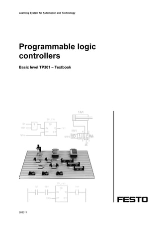
Sorting station task
Various parts for built-in kitchens are to be machined in a production
system (milling and drilling machine). The wall and door sections for
certain types of kitchen are to be provided with different drill holes. Sen-
sors B1 to B4 are intended for the detection of the holes.
B1
B2
B3
B4
1A1
Parts with the following hole patterns are for the ’Standard’ kitchen type.
These parts are to be advanced via the double-acting cylinder 1.0.
Fig. B3.11:
Sorting station

B-26
Chapter 3
b d
a
d
a
b d
d
a c
b d
a c
d
Assuming that a drilled hole is read as a 1-signal, the following truth ta-
ble results.
a b c d y
0 0 0 0 0
0 0 0 1 1
0 0 1 0 0
0 0 1 1 0
0 1 0 0 0
0 1 0 1 1
0 1 1 0 0
0 1 1 1 0
1 0 0 0 0
1 0 0 1 1
1 0 1 0 0
1 0 1 1 1
1 1 0 0 0
1 1 0 1 1
1 1 1 0 0
1 1 1 1 1
Fig. B3.12:
Hole pattern parts
Fig. B3.13
Truth table

B-27
Chapter 3
Two options are available in order to derive the logic equation from this
table, which lead to two different expressions. The same result is ob-
tained, of course, since the same circumstances are described.
Standard form, disjunctive
In the disjunctive standard form, all conjunctions (AND-operations) of
input variables with the result 1, are carried out as a disjunctive opera-
tion (OR-operation). With signal status 0, the input variable is carried out
as a negated operation and with signal status 1 as a non-negated opera-
tion.
In the case of the example given, the logic operation is therefore as fol-
lows:
y = ( ) ( ) ( )∨∧∧∧∨∧∧∧∨∧∧∧ dcbadcbadcba
( ) ( ) ( )dcbadcbadcba ∧∧∧∨∧∧∧∨∧∧∧
Conjunctive standard form
In the conjunctive standard form, all disjunctions (OR-operations) of the
input variable producing the result 0, are carried out as a conjunctive
operation (AND-operation). In contrast with the disjunctive standard
form, in this instance, the input variable is negated with signal status "1"
and a non-negated operation carried out with signal status "0".
y = ( ) ( ) ( )∧∨∨∨∧∨∨∨∧∨∨∨ dcbadcbadcba
( ) ( ) ( )∧∨∨∨∧∨∨∨∧∨∨∨ dcbadcbadcba
( ) ( )∧∨∨∨∧∨∨∨ dcbadcba
( ) ( )dcbadcba ∨∨∨∧∨∨∨

B-28
Chapter 3
3.4 Simplification of logic functions
Both equations for the example given are rather extensive, with that of
the conjunctive standard form being even longer still. This defines the
criteria for using the disjunctive or conjunctive standard from: The deci-
sion is made in favour of the shorter form of the equation. In this case,
the disjunctive standard form.
y = ( ) ( ) ( )∨∧∧∧∨∧∧∧∨∧∧∧ dcbadcbadcba
( ) ( ) ( )dcbadcbadcba ∧∧∧∨∧∧∧∨∧∧∧
This expression may be simplified with the help of a boolean algorithm.
The most important rules in boolean algebra are shown below:
a0a =∨ 00a =∧
11a =∨ a1a =∧
aaa =∨ aaa =∧
1aa =∨ 0aa =∧
Commutative law
abba ∨=∨ abba ∧=∧
Associative law
( ) ( ) cbacbacba ∨∨=∨∨=∨∨
( ) ( ) cbacbacba ∧∧=∧∧=∧∧

B-29
Chapter 3
Distributive law
( ) ( ) ( )cabacba ∧∨∧=∨∧ ( ) ( ) ( )cabacba ∨∧∨=∧∨
De Morgan’s rule
baba ∧=∨ baba ∨=∧
Reduction rule
babaa ∨=∧∨
Applied to the above example, the following result is obtained:
y = abcddcabcdbadbcadcbadabc ∨∨∨∨∨
= ( )ccabdcdbadbcadcbadabc ∨∨∨∨∨
= ( ) ( ) abdccdbabbdac ∨∨∨∨
= abddbadac ∨∨
= ( )bbaddac ∨∨
= ( )daac ∨
= ( )dac ∨
= addc ∨
For reasons of clarity, the AND-operation symbol “∧”has been omitted in
the individual expressions.
The basic principle of simplification is in the factoring out of variables
and reducing to defined expressions. However, this method does require
a sound knowledge of boolean algorithms plus a certain amount of prac-
tice. Another option for simplification will be introduced in the following
section.

B-30
Chapter 3
3.5 Karnaugh-Veitch diagram
In the case of the Karnaugh-Veitch diagram (KV diagram) the truth table
turns into a value table.
a b c d y No.
0 0 0 0 0 1
0 0 0 1 1 2
0 0 1 0 0 3
0 0 1 1 0 4
0 1 0 0 0 5
0 1 0 1 1 6
0 1 1 0 0 7
0 1 1 1 0 8
1 0 0 0 0 9
1 0 0 1 1 10
1 0 1 0 0 11
1 0 1 1 1 12
1 1 0 0 0 13
1 1 0 1 1 14
1 1 1 0 0 15
1 1 1 1 1 16
A total of 16 allocation options are available for the example, whereby
the value table must also have 16 squares.
cd dc dc cd
ab 1 2 3 4
ba 5 6 7 8
ba 9 10 11 12
ab 13 14 15 16
Fig. B3.14:
Truth table
Fig. B3.15:
Value table

B-31
Chapter 3
The results of the value table are transferred to the KV diagram accord-
ing to the diagram shown below. In principle, representation is again
possible in conjunctive or disjunctive standard form. The following, how-
ever, will be limited to the disjunctive standard form.
cd dc dc cd
ab 0 1 0 0
ba 0 1 0 0
ba 0 1 0 1
ab 0 1 0 1
The next step consists of combining the statuses, for which "1" has been
entered in the value table. This is done in blocks whilst observing the
following rules:
The combining statuses in the KV diagram must be in the form of a
rectangle or square
The number of combining statuses must be a result of function 2x
.
This results in the following:
cd dc dc cd
ab 0 1 0 0
ba 0 1 0 0
ba 0 1 0 1
ab 0 1 0 1
Fig. B3.16:
Value table
Fig. B3.17:
Value table
Y1 Y2

B-32
Chapter 3
The variable values are selected for the established block and these in
turn combined disjunctively.
y1 = dc
y2 = acd
y = acddc ∨
= ( ) dacc ∧∨
= ( ) dac ∧∨
= addc ∨
Naturally, the KV diagram is not limited to 16 squares. 5 variables, for
instance, would result in 32 squares (25
), and 6 variables 64 fields (26
).

B-33
Chapter 4
Design and mode of operation of a PLC
4.1 Structure of a PLC
With computer systems, differentiation is generally made between hard-
ware, firmware and software. The same applies for a PLC, which is es-
sentially based on a microcomputer.
The hardware consists of the actual device technology, i.e. the printed
circuit boards, integrated modules, wires, battery, housing, etc.
Firmware is the software part, which is permanently installed and sup-
plied by the PLC manufacturer. This includes fundamental system rou-
tines, used for starting the processor after the power has been switched
on. Additionally, there is the operating system in the case of program-
mable logic controllers, which is generally stored in a ROM, a read-only
memory, or in the EPROM.
Finally, there is the software, which is the user program written by the
PLC user. User programs are usually installed in the RAM, a random
access memory, where they can be easily modified.
Micro-
pro-
cessor
(CPU)
Address bus
Operating-
system
Input-
module
ROM
Program
and data
RAM Output-
module
Control bus
Data bus
Fig. B4.1:
Fundamental design
of a microcomputer

B-34
Chapter 4
Fig. B4.1 illustrates the fundamental design of a microcomputer. PLC
hardware – as in the case of almost all of today’s microcomputer sys-
tems – is based on a bus system. A bus system is a number of electrical
lines divided into address, data and control lines. The address line is
used to select the address of a connected bus station and the data line
to transmit the required information. The control lines are necessary to
activate the correct bus station either as a transmitter or sender.
The major bus stations connected to the bus system are the microproc-
essor and the memory. The memory can be divided into memory for the
firmware and memory for the user program and data.
Depending on the structure of the PLC, the input and output modules
are connected to a single common bus or – with the help of a bus inter-
face – to an external I/O bus. Particularly in the case of larger modular
PLC systems, an external I/O bus would be more usual.
Finally, a connection is required for a programming device or a PC,
nowadays mostly in the form of a serial interface.
Fig. B4.2 illustrates the Festo FPC 101 as an example.
Fig. B4.2:
Programmable logic control-
ler Festo FPC 101

B-35
Chapter 4
4.2 Central control unit of a PLC
In essence, the central control unit of a PLC consists of a microcom-
puter. The operating system of the PLC manufacturer makes the univer-
sal computer into a PLC, optimised specifically for control technology
tasks.
Design of the central control unit
Fig. B4.3 illustrates a simplified version of a microprocessor, which
represents the heart of a microcomputer.
Command register
Program counter
Control bus
ALU
Accumulator
Arithmetic unit Control unit
Control bus
Address bus
Data bus
A microprocessor consists in the main of an arithmetic unit, control unit
and a small number of internal memory units, so-called registers.
The task of the arithmetic unit – the ALU (arithmetic logic unit) – is to
execute arithmetic and logic operations with the data transmitted.
The accumulator, AC for short, is a special register assigned directly to
the ALU. This stores both data to be processed as well as the result of
an operation.
The instruction register stores a command called from the program
memory until this is decoded and executed.
A command consists of an operation part and an address part. The op-
eration part indicates which logic operation is to be carried out. The ad-
dress part defines the operands (input signals, flags etc.), with which a
logic operation is to be executed.
Fig. B4.3:
Design of a
microprocessor

B-36
Chapter 4
The program counter is a register, which contains the address of the
next command to be processed. The following section will be dealing
with this in greater detail.
The control unit regulates and controls the entire logic sequence of the
operations required for the execution of a command.
Instruction cycle within central control unit
Today’s conventional microcomputer systems operate according to the
so-called "von-Neumann principle". According to this principle, the com-
puter processes the program line by line. In simple terms, you could say
that each program line of the PLC user program is processed in se-
quence.
This applies wholly irrespective of the programming language, in which
the PLC program is written, be it in the form of a text program (statement
list) or a graphic program (ladder diagram, sequential function chart).
Since these various forms of representation always result in a series of
program lines within the computer, they are subsequently processed one
after the other.
In principle, a program line, i.e. generally a command, is processed in
two steps:
fetching the command from the program memory
executing the command
+1
Memory
Addresses
Command Command
register
Control signals
Program-
counter
Microprocessor
Command
Address bus
Data bus
Fig. B4.4:
Command sequence

B-37
Chapter 4
The contents of the program counter are transferred to the address bus.
The control unit then causes the command at a specified address in the
program memory, to be relayed to the data bus. From there, the com-
mand is read to the instruction register. Once the command has been
decoded, the control unit generates a sequence of control signals for
execution.
During the execution of a program, the commands are fetched in se-
quence. A mechanism, which permits this sequence, is therefore re-
quired. This task is performed by a simple incrementer, i.e. a step
enabling facility in the program counter.
4.3 Function mode of a PLC
Programs for conventional data processing are processed once only
from top to bottom and then terminated. In contrast with this, the pro-
gram of a PLC is continually processed cyclically.
Inputs
Image table
Inputs
PLC program
Image table
Outputs
Outputs
Fig. B4.5:
Cyclical processing of
a PLC program

B-38
Chapter 4
The characteristics of cyclical processing are:
As soon as the program has been executed once, it automatically
jumps back to the beginning and processing is repeated.
Prior to first program line being processed, i.e. at the beginning of the
cycle, the status of the inputs is stored in the image table. The proc-
ess image is a separate memory area accessed during a cycle. The
status of an input thus remains constant during a cycle even if it has
physically changed
Similar to inputs, outputs are not immediately set or reset during a
cycle, but the status stored intermediately in the process output im-
age. Only at the end of a cycle are all the outputs physically switched
according to the logic status stored in the memory.
The processing of a program line via the central control unit of a PLC
takes time which, depending on PLC and operation can vary between a
few microseconds and a few milliseconds.
The time required by the PLC for a single execution of a program includ-
ing the actualisation and output of the process image, is termed the cy-
cle time. The longer the program is and the longer the respective PLC
requires to process an individual program line, the longer the cycle. Re-
alistic time periods for this are between approximately 1 and 100 milli-
seconds.
The consequences of cyclical processing of a PLC program using a
process image are as follows:
Input signals shorter than the cycle time may possibly not be recog-
nised.
In some cases, there may be a delay of two cycle times between the
occurrence of an input signal and the desired reaction of an output to
this signal.
Since the commands are processed sequentially, the specific behav-
iour sequence of a PLC program may be crucial.
With some applications it is essential for inputs or outputs to be ac-
cessed directly during a cycle. This type of program processing, bypass-
ing of the process image, is therefore also supported by some PLC
systems.

B-39
Chapter 4
4.4 Application program memory
Programs specifically developed for particular applications require a
program memory, from which these can be read cyclically by the central
control unit. The requirements for such a program memory are relatively
simple to formulate:
It should be as simple as possible to modify or to newly create and
store the program with the help of a programming device or a PC
Safeguards should be in place to ensure that the program cannot be
lost – either during power failure or through interference voltage
The program memory should be cost effective
The program memory should be sufficiently fast in order not to delay
the operation of the central control unit.
Nowadays, three different types of memory are used in practice:
RAM
EPROM
EEPROM
RAM
The RAM (random access memory) is a fast and highly cost effective
memory. Since the main memory of computers (i.e. PLCs) consist of
RAMs, they are produced in such high quantities that they are readily
available at low cost without competition.
RAMs are read/write memories and can be easily programmed and
modified.
The disadvantage of a RAM is that it is volatile, i.e. the program stored in
the RAM is lost in the event of power failure. This is why RAMs are
backed up by battery or accumulator. Since the service life and capacity
of modern batteries are rated for several years, RAM back-up is rela-
tively simple. Despite the fact that these are high performance batteries
it is nevertheless essential to replace the batteries in good time.

B-40
Chapter 4
EPROM
The EPROM (erasable programmable read-only memory) is also a fast
and low cost memory, which, in comparison with RAM, has the added
advantage of being non-volatile, i.e. remanent. The memory contents
therefore remain intact even in the event of power failure.
For the purpose of a program modification, however, the entire memory
must first be erased and, after a cooling period, completely repro-
grammed. Erasing generally requires an erasing device, and a special
programming unit is used for programming.
Despite this relatively complex process of erasing, – cooling – repro-
gramming EPROMs are very frequently used in PLCs, since these rep-
resent reliable and cost effective memories. In practice, a RAM is often
used during the programming and commissioning phase of a machine.
On completion of the commissioning, the program is then transferred to
an EPROM.
EEPROM
The EEPROM (electrically erasable programmable ROM), EEROM
(electrically erasable ROM) and EAROM (electrically alterable ROM) or
also flash-EPROM have been available for some time. The EEPROM in
particular, is used widely as an application memory in PLCs. The
EEPROM is an electrically erasable memory, which can be subse-
quently written to.
Fig. B4.6:
Example of an EPROM

B-41
Chapter 4
4.5 Input module
The input module of a PLC is the module, which sensors are connected
to. The sensor signals are to be passed on to the central control unit.
The important functions of an input module (for the application) are as
follows:
Reliable signal detection
Voltage adjustment of control voltage to logic voltage
Protection of sensitive electronics from external voltages
Screening of signals
Error
voltage
detection
Signal
delay
Optocoupler Signal to
the
control unit
Input-
signal
The main component of today’s input modules which meets these re-
quirements is the optocoupler.
The optocoupler transmits the sensor information with the help of light,
thereby creating an electrical isolation between the control and logic
circuits, thereby protecting the sensitive electronics from spurious ex-
ternal voltages. Nowadays, advanced optocouplers guarantee protection
for up to approximately 5 KV, which is adequate for industrial applica-
tions.
The adjustment of control and logic voltage, in the straightforward
case of a 24 V control voltage, can be effected with the help of a break-
down diode/resistor circuit. In the case of 220 V AC, a rectifier is con-
nected in series.
Depending on PLC manufacturer reliable signal detection is ensured
either by means of an additional downstream threshold detector or a
corresponding range of breakdown diodes and optocouplers. Precise
data regarding the signals to be detected is specified in DIN 19 240.
Fig. B4.7:
Block diagram of an
input module

B-42
Chapter 4
The screening of the signal emitted by the sensor is critical in industrial
automation. In industry, electrical lines are generally loaded heavily due
to inductive interference voltages, which leads to a multitude of interfer-
ence impulses on every signal line. Signal lines can be screened either
via shielding, discrete cable ducts etc, or alternatively the input module
of the PLC assumes the screening via an input signal delay.
This therefore requires the input signal to be applied for a sufficiently
long period, before it is even recognised as an input signal. Since, due
to their inductive nature, interference impulses are primarily transient
signals, a relatively short input signal delay of a few milliseconds is suffi-
cient to filter out most of the interference impulses.
Input signal delay is effected mainly via the hardware, i.e. via connection
of the input to an RC module. In isolated cases, however, it is also pos-
sible to produce an adjustable signal delay via the software.
The duration of an input signal delay is approximately 1 to 20 millisec-
onds – depending on manufacturer and type. Most manufacturers offer
especially fast inputs for tasks, where the input signal delay is then too
long to recognise the required signal.
Differentiation is made between positive and negative switching connec-
tions when connecting sensors to PLC inputs. In other words, differentia-
tion is made between inputs representing a current sink or a current
source. In Germany for instance positive switching connections are
mainly used, since this permits the use of protective grounding. Positive
switching means that the PLC input represents a current sink. The sen-
sor supplies the operating voltage or control voltage to the input in the
form of a 1-signal.
If protective grounding is employed, the output voltage of the sensor is
short-circuited towards 0 volts or the fuse switched off in the event of a
short-circuit in the signal line. This means that a logic 0 is applied at the
input of the PLC.

B-43
Chapter 4
In a number of countries, the use of negative switching sensors is com-
monplace, i.e. the PLC inputs operate as a power source. In these
cases, a different protective measure must be used to prevent a 1-signal
from being applied to the input of the PLC in the event of a shortcircuit
on the signal line. Possible methods are the earthing of the positive con-
trol voltage or insulation monitoring, i.e. protective grounding as a pro-
tective measure.
4.6 Output module
Output modules conduct the signals of the central control unit to final
control elements, which are actuated according to the task. In the main,
the function of an output – as seen from the application of the PLC –
therefore includes the following:
Voltage adjustment of logic voltage to control voltage
Protection of sensitive electronics from spurious voltages from the
controller
Power amplification sufficient for the actuation of major final control
elements
Short-circuit and overload protection of output modules
In the case of output modules, two fundamentally different methods are
available to achieve the above: Either the use of a relay or power elec-
tronics.
Signal from
the
control unit
Output
signal
Short-circuit
monitoring
Amplifier
Optocoupler
The optocoupler once again forms the basis for power electronics and
ensures the protection of the electronics and possibly also the voltage
adjustment.
A protective circuit consisting of diodes must protect the integral power
transistor from voltage surges.
Fig. B4.8:
Block diagram of an
output module

B-44
Chapter 4
Nowadays short-circuit protection, overload protection and power
amplification are often ensured with fully integral modules. Standard
short-circuit protection measures the current flow via a power resistor so
as to switch off in the event of short-circuit; a temperature sensors pro-
vides overload protection; a Darlington stage or alternative power tran-
sistor stages provide the necessary power.
The permissible power of an output module is usually specified in a way,
which permits differentiation to be made between the permissible power
of an output and the permissible cumulative power of an output module.
The cumulative power of a module is almost always considerably lower
than the total of individual permissible ratings, since power transistors
transmit heat to one another.
If relays are used for the outputs, then the relay can assume practically
all the functions of an output module: The relay contact and relay coil are
electrically isolated from one another; the relay represents an excellent
power amplifier and is particularly overload-proof, only short-circuit pro-
tection must be ensured via an additional fuse. In practice, however,
optocouplers are nevertheless connected in series with relays, since this
renders the actuation of relays easier and simpler relays can be used.
Relay outputs have the advantage that they can be used for different
output voltages. By contrast, electronic outputs have considerably higher
switching speeds and a longer service life than relays. In most cases,
the power of the very small relays used in PLCs corresponds to that of
the power stages of electronic outputs.
In Germany for example, outputs are also connected positive switching,
i.e. the output represents a power source and supplies the operating
voltage to the consuming device.
In the case of a short circuit of the output signal line to earth, the output
is short-circuited, if normal protective grounding measures are used. The
electronics switch to short circuit protection or the fuse switches off, i.e.
the consuming device cannot draw any current and is therefore uncon-
nected and rendered safe. (In accordance with EN 60204, the deener-
gised status must always be the safe status).
If negative switching outputs are used, i.e. the output represents a cur-
rent sink, the protective measure must be adapted in such a way, that
the consuming device is rendered safe in the event of a short circuit on
the signal line. Again, protective grounding with isolation monitoring or
the neutralising of the positive control voltage are standard practice in
this case.

B-45
Chapter 4
4.7 Programming device/Personal computer
Each PLC has a programming and diagnostic tool in support of the PLC
application.
Programming
Testing
Commissioning
Fault finding
Program documentation
Program storage
These programming and diagnostic tools are either vendor specific pro-
gramming devices or personal computers with corresponding software.
Nowadays, the latter is almost exclusively the preferred variant, since
the enormous capacity of modern PCs, combined with their compara-
tively low initial cost and high flexibility, represent crucial advantages.
Also available and being developed are so-called hand-held program-
mers for mini control systems and for maintenance purposes. With the
increasing use of laptop personal computers, i.e. portable, battery oper-
ated PCs, the importance of hand-held programmers is steadily decreas-
ing.
Essential software system functions forming part of the program-
ming and diagnostic tool
Any programming software conforming to EN 61131-1 (IEC 61131-1)
should provide the user with a series of functions. Hence the program-
ming software comprises software modules for:
Program input
Creating and modifying programs in one of the programming lan-
guages via a PLC.
Syntax test
Checking the input program and the input data for syntax accuracy,
thus minimizing the input of faulty programs.
Translator
Translating the input program into a program, which can be read and
processed by the PC, i.e. the generation of the machine code of the
corresponding PC.
Connection between PLC and PC
This data circuit effects the loading of a program to the PLC and the
execution of test functions.

B-46
Chapter 4
Test functions
Supporting the user during writing and fault elimination and checking
the user program via
– a status check of inputs and outputs, timers, counters etc.
– testing of program sequences by means of single-step operations,
STOP commands etc.
– simulation by means of manual setting of inputs/outputs, setting
constants etc.
Status display of control systems
Output of information regarding machine, process and status of the
PLC system
– Status display of input and output signals
– Display/recording of status changes in external signals and inter-
nal data
– Monitoring of execution times
– Real-time format of program execution
Documentation
Drawing up a description of the PLC system and the user program.
This consists of
– Description of the hardware configuration
– Printout of the user program with corresponding data and identifi-
ers for signals and comments
– Cross-reference list for all processed data such as inputs, outputs,
timers etc.
– Description of modifications
Archiving of user program
Protection of the user program in nonvolatile memories such as
EPROM etc.

B-47
Chapter 5
Programming of a PLC
5.1 Systematic solution finding
Control programs represent an important component of an automation
system.
Control programs must be systematically designed, well structured and
fully documented in order to be as
error-free
low-maintenance
cost effective
as possible.
Phase model of PLC software generation
The procedure for the development of a software program illustrated in
fig. B5.1 has been tried and tested. The division into defined sections
leads to targeted, systematic operation and provides clearly set out re-
sults, which can be checked against the task.
The phase model consisting of the following sections
Specification: Description of the task
Design: Description of the solution
Realisation: Implementation of the solution
Integration/commissioning: Incorporating into environment and testing
the solution
can be applied to basically all technical projects. Differences occur in the
methods and tools used in the individual phases.

B-48
Chapter 5
– Macrostructure of control program
Commissioning
Specification1.
2.
3.
4.
– Verbal description of control task
– Technology, positional sketch
Design – Function chart to IEC 60848
– Logic chart with symbols of the
EN 60617-12 (IEC 60617)
– Function table
– Definition of software modules
– Part list and circuit diagram
Realisation – Programming in LD, FBD, IL,
ST and SFC
– Simulation of subprograms and
overall program
– Design of system
– Testing of subprograms
– Testing of overall program
The phase model can be applied to control programs of varying com-
plexity; for complex control tasks the use of such a model is absolutely
essential.
The individual phases of the model are described below.
Phase 1: Specification (Problem formulation)
In this phase, a precise and detailed description of the control task is
formulated. The specific description of the control system function, for-
malised as much as possible, reveals any conflicting requirements, mis-
leading or incomplete specifications.
The following are available at the end of this phase:
Verbal description of the control task
Structure/layout
Macrostructuring of the system or process and thus rough structuring
of the solution
Fig. B5.1:
Phase model for the
generation of PLC software

B-49
Chapter 5
Phase 2: Design (Concrete form of solution concept)
A solution concept is developed on the basis of the definitions estab-
lished in phase 1. The method used to describe the solution must pro-
vide both a graphic and process oriented description of the function and
behaviour of the control system and be independent of the technical
realisation.
These requirements are fulfilled by the function chart (FCH) as defined
in IEC 60848. Starting with a representation of the overall view of the
controller (rough structure of the solution), the solution can be refined
step by step until a level of description is obtained, which contains all the
details of the solution (refinement of rough structure).
In the case of complex control tasks, the solution is structured into indi-
vidual software modules in parallel with this. These software modules
implement the job steps of the control system. These can be special
functions such as the realisation of an interface for visualisation or com-
munications systems, or equally permanently recurring job steps.
Phase 3: Realisation (Programming of solution concept)
The translation of the solution concept into a control program is effected
via the programming languages defined in EN 61131-3 (IEC 61131-3).
These are: sequential function chart, function block diagram, ladder dia-
gram, statement list and structured text.
Control systems operating in a time/logic process and available in func-
tion chart to IEC 60848, can be clearly and easily programmed in a se-
quential function chart. A sequential function chart, in as far as possible,
uses the same components for programming as those used for the de-
scription in the function chart to IEC 60848.
Ladder diagram, function block diagram and statement list are the pro-
gramming languages suitable for the formulation of basic operations and
for control systems which can be described by simple operations logic
operations or boolean signals.
The high-level language structured text is mainly used to create software
modules of mathematical content, such as modules for the description of
control algorithms.

B-50
Chapter 5
In so far as PLC programming systems support this, the control pro-
grams or parts of a program created should be simulated prior to com-
missioning. This permits the detection and elimination of errors right at
the initial stage.
Phase 4:
Commissioning (Construction and testing of the control task)
This phase tests the interaction of the automation system and the con-
nected plant. In the case of complex tasks, it is advisable to commission
the system systematically, step by step. Faults, both in the system and
in the control program, can be easily found and eliminated using this
method.
Documentation
One important and crucial component of a system is documentation,
which is an essential requirement for the maintenance and expansion of
a system. Documentation, including the control programs, should be
available both on paper and on a data storage medium.
The documentation consists of the document of the individual phases,
printouts of the control programs and of any possible additional descrip-
tions concerning the control program. Individually these are:
Problem description
Positional sketch or technology pattern
Circuit diagram
Terminal diagram
Printouts of control programs in SFC, FBD etc..
Allocation list of inputs and outputs (this also forms part of the control
program printouts)
Additional documentation
5.2 EN 61131-3 (IEC 61131-3) structuring resources
EN 61131-3 (IEC 61131-3) is a standard for the programming of not just
one individual PLC, but primarily also of complex automation systems.
Control programs for extensive applications must be clearly structured in
order to be intelligible, maintainable and possibly also portable, i.e.
transferable to another PLC system.

B-51
Chapter 5
Definitions are required not only for elementary language commands,
but also for the language elements for structuring. Structuring resources
(fig. B5.2) relate to the control programs and the configuration of the
automation system.
– Configuration
automation system
CONFIGURATION
RESOURCE
TASK
VAR_GLOBAL
ACCESS_PATH
Structuring
of
configuration
level
Structuring
of
program level
– Sequence
representation
– Refinement
Sequential function
chart
– Modularisation
PROGRAM
FUNCTION_BLOCK
FUNCTION
DATATYPES
Structuring resources at program level
The structuring resources – program, function block and function – con-
tain the actual control logic (rules) of the control program. These are also
known as program organisation units. These structuring resources are
available for any programming language. They are used for the modu-
larization of control programs and the user program – this concerns pri-
marily programs and function blocks – or also supplied by the
manufacturer – as far as programs, function blocks are concerned.
EN 61131-3 (IEC 61131-3) defines a comprehensive set of standardised
functions and function block. These can be expanded by own user func-
tions and function block for special or continually recurring tasks.
Software modules, which can be used in any way, are entered in librar-
ies, where they are made available.
Programs represent the outer program organisation shell and can be
differentiated from the function block mainly by the fact that they cannot
be invoked by any other program organisation unit.
The sequential function chart represents another resource for structuring
at program level. The contents of the actual programs and function block
can again be clearly and intelligibly represented by means of a sequen-
tial function chart.
Fig. B5.2:
EN 61131-3
(IEC 61131-3)
structuring method

B-52
Chapter 5
Structuring resources at configuration level
The language elements for configuration describe the incorporation of
control programs in the automation system and their time-related control.
The automation system represents a configuration (CONFIGURATION
language element). Within the configuration, there are global variables
VAR_GLOBAL language element).
A resource (RESOURCE language element) corresponds to the proces-
sor of a multiprocessor system, to which one or several programs are
assigned. In addition, it comprises control elements, which include the
time-related control of programs. This control element is a task (TASK
language element). The control element Task defines whether a pro-
gram is to be processed cyclically or once only, triggered by a specific
event. Programs not specifically linked to a task are processed cyclically
in the background and with the lowest priority.
Configuration
Valve_production
Task_1 Task_2
Program
Assembly
Program
Initial_position_run
Program
Conveyor
Program
Conveyor_idle_run
Resource
Conveyor_control
Task_
cyclical
Program
Packaging
Resource
Quality_control
Task_
unique
Program
Statistics
Program
Data_save
Global and directly represented variables
Resource
Valve_assembly
The structuring resources for configuration are shown in a combined
overview in fig. B5.3. An example applying these to an automation task
is given by way of an explanation.
The task in hand is to design and automate a production line for the as-
sembly of pneumatic valves.
Fig. B5.3:
Graphic example
of a configuration

B-53
Chapter 5
A PLC multiprocessor with three processor cards has been designated
for the valve assembly. The processor cards are assigned to the
valve_assembly, the conveyor control and quality_control.
The programs Statistics and Data_save are associated with different
tasks. As such they possess different execution characteristics. The
program Statistics evaluates and compresses the quality data at regular
intervals. The priority of this program is low. It is started regularly, e.g.
every 20 minutes, by the task Task_cyclical. In the event of an
EMERGENCY- STOP, the program Data_save is to transmit all available
data to a higher-order cell computer in order to prevent any potential
data loss. The program is started event-driven of the highest priority via
the EMERGENCY-STOP signal.
EN 61131-3 (IEC 61131-3) provides defined and thus standardised inter-
faces for the exchange of data within a configuration. If specific informa-
tion such as a read variable, is required in different program organisation
units, this variable is designated as a global variable. Data can then be
exchanged via a variable designated as such. Global variables can only
be accessed in programs and function blocks.
What is of interest for networked systems is communication beyond a
configuration. Special standard communication function blocks are
available to the user for this. These are defined in EN 61131-5 (IEC
61131-5) and are used in EN 61131-3 (IEC 61131-3). Another possibility
is the definition of access paths (language resource ACCESS_PATH) to
specific variables. These can then also be read or written from other
positions.

B-54
Chapter 5
5.3 Programming languages
EN 61131-3 (IEC 61131-3) defines five programming languages. Al-
though the functionality and structure of these languages is very differ-
ent, these are treated as one language family by EN 61131-3 (IEC
61131-3) with overlapping structure elements (variable declaration, or-
ganisation parts such as function and function block, etc.) and configura-
tion elements.
The languages can be mixed in any way within a PLC project. The unifi-
cation and standardisation of these five languages represent a compro-
mise of historical, regional and branch-specific requirements. Provision
has been made for future expansion, (such as the function block princi-
ple or the language Structured Text) plus necessary information tech-
nology details (data type etc.) have been incorporated.
The language elements are explained with the help of a machining proc-
ess involved in valve production. Two sensors are used to establish
whether a workpiece with correctly drilled holes is available at the ma-
chining position. If the valve to be machined is of type A or type B – this
is set via two selector switches – the cylinder advances and presses the
sleeve into the drilled hole.
Ladder diagram (LD)
Ladder diagram is a graphic programming language derived from the
circuit diagram of directly wired relay controls. The ladder diagram con-
tains contact rails to the left and the right of the diagram; these contact
rails are connected to switching elements (normally open/normally
closed contacts) via current paths and coil elements.
Part_TypeA Part_present Drill_ok Sleeve_in
Part_TypeB
Fig. B5.4:
Example of ladder
diagram language

B-55
Chapter 5
Function block diagram (FBD)
In the function block diagram, the functions and function blocks are rep-
resented graphically and interconnected into networks. The function
block diagram originates from the logic diagram for the design of elec-
tronic circuits.
OR
Part_TypeB
AND Sleeve_in
Part_present
Drill_ok
Part_TypeA
Instruction list (IL)
Instruction list is a textual assembler-type language characterised by a
simple machine model (processor with only one register). Instruction list
is formulated from control instructions consisting of an operator and an
operand.
LD Part_TypeA
OR Part_TypeB
AND Part_present
AND Drill_ok
ST Sleeve_in
With regard to language philosophy, the ladder diagram, the function
block diagram and instruction list have been defined in the way they are
used in today’s PLC technology. They are however limited to basic func-
tions as far as their elements are concerned. This separates them es-
sentially from the company dialects used today. The competitiveness of
these languages is maintained due to the use of functions and function
blocks.
Fig. B5.5:
Example of function block
diagram language
Fig. B5.6:
Example of instruction
list language

B-56
Chapter 5
Structured text (ST)
Structured text is high-level language based on Pascal, which consists
of expressions and instructions. Instructions can be defined in the main
as: Selection instructions such as IF...THEN...ELSE etc., repetition in-
structions such as FOR, WHILE etc. and function block invocations.
Sleeve_in := (Part_TypeA OR Part_TypeB) AND Part_present AND Drill_ok;
Structured text enables the formulation of numerous applications, be-
yond pure function technology, such as algorithmic problems (high order
control algorithms etc.) and data handling (data analysis, processing of
complex data structures etc.).
Sequential function chart (SFC)
The sequential function chart is a language resource for the structuring
of sequence-oriented control programs.
The elements of the sequential function chart are steps, transitions, al-
ternative and parallel branching.
Each step represents a processing status of a control program, which is
active or inactive. A step consists of actions which, identical to the tran-
sitions, are formulated in the EN 61131-3 (IEC 61131-3) languages. Ac-
tions themselves can again contain sequence structures. This feature
permits the hierarchical structure of a control program. The sequential
function chart is therefore an excellent tool for the design and structuring
of control programs.
Fig. B5.7:
Example of structured text
language

B-57
Chapter 6
Common elements of programming languages
6.1 Resources of a PLC
According to EN 61131-3 (IEC 61131-3), only inputs and outputs and the
controller memory can be addressed directly by a control program. Di-
rect addressing in this instance means that in the program an input, out-
put or memory element of the controller is affected immediately and not
indirectly via a defined symbolic variable. Naturally, EN 61131-3 (IEC
61131-3) recognises numerous other resources, e.g. timers and count-
ers. However, these are integrated into functions and function blocks in
order to ensure the highest possible degree of control program portabil-
ity between different control systems.
Inputs, outputs and the memory
The most important controller constituents include the inputs, outputs
and the memory. Only via its inputs can a controller receive information
from the connected processes. Similarly it can only influence these via
its outputs or store information for subsequent continued processing.
The designations for the resources inputs, outputs and memory ele-
ments are defined by EN 61131-3 (IEC 61131-3) and mandatory.
Inputs I
Outputs Q
Memory M
Without further reference, these designate only binary inputs or outputs
and single bit memory elements, designated as a flag.
The standard generally speaks of directly represented variables. These
are variables, which are referred directly to the hardware-related avail-
able inputs, outputs and memory elements of the controller. The alloca-
tion of inputs, outputs and flags and their physical or logical position in
the control system is defined by the respective controller manufacturer.
Fig. B6.1:
Designations for
inputs, outputs
and memory

B-58
Chapter 6
Insofar as the controller supports this, resources can be addressed,
which are defined in excess of one bit. EN 61131-3 (IEC 61131-3) em-
ploys a further letter to describe this, which follows the abbreviation I, Q
or M and, for instance, designates bytes and words.
EN 61131-3 (IEC 61131-3) designates the data types shown in fig. B6.2
in conjunction with inputs, outputs and flags.
BOOL Bit sequence of length 1
BYTE Bit sequence of length 8
WORD Bit sequence of length 16
1-Bit sizes, such as defined by the data type BOOL (boolean), may only
assume the values 0 or 1. Consequently, the range of values for BOOL
type data consists of the two values 0 and 1.
In contrast with this, one should observe that in the case of bit sequence
data types consisting of more than one bit, there is no immediate con-
nected range of values. All bit sequence data types such as for instance
BYTE and WORD are merely a combination of several bits. Each of
these bits has the value 0 or 1, but their combination does not have its
own value.
The mandatory designation methods for inputs, outputs and flags of dif-
ferent bit length are represented in fig. B6.3.
I, Q, M or
IX, QX, MX
Input bit, output bit, memory bit 1 Bit
IB, QB, MB Input byte, output byte, memory byte 8 Bit
IW, QW, MW Input word, output word, memory word 16 Bit
An individual bit of an input, output or flag may also be addressed with-
out the additional abbreviation X for the data type.
Fig. B6.2:
Data types
Fig. B6.3
Designations for inputs,
outputs and memory

B-59
Chapter 6
Since a controller always has a relatively large number of inputs, outputs
and flags available, these must be specially identified for the purpose of
differentiation. Numbering is used in EN 61131-3 (IEC 61131-3) to this
end, such as in the following example:
I1 Input 1
IX9 Input 9
I15 Input 15
QW3 Output word3
MB5 Memory byte 5
MX2 Memory 2
EN 61131-3 (IEC 61131-3) does not specify the number range, which is
permissible for this numbering and whether it should start with 0 or 1.
This is specified by the controller manufacturer.
A hierarchical number of inputs, outputs and flags may also be used, if
the controller in use has been suitably configured.
A point is used to separate the individual levels of the hierarchy. The
number of hierarchy levels has not been defined.
In the case of hierarchical numbering, the highest position in the number
on the left must be coded, the numbers further to the right represent
consecutive lower positions.
I3.8.5
The specified input I3.8.5 can therefore be be made up as follows:
Input
in insert No. 3
on plug-in card No. 8
as input No. 5
I 3. 8. 5
Example
Fig. B6.4:
Structure of a
hierarchical designation

B-60
Chapter 6
EN 61131-3 (IEC 61131-3) does not make any comment regarding the
assignment of individual bits in a BYTE or WORD. Controller manufac-
turers frequently choose hierarchical designation methods to assign in-
dividual bits as parts of words. As such, F6.2 could for instance
represent the bit number 2 of flag word number 6. However, this does
not necessarily have to be so, since flag bit F6.2 and flag word FW6
need not be in any way connected. Moreover, no definition has been
made as to whether the numbering of individual bits in one word is to
start on the left or the right (bit number 0 on the far right has been the
most frequently used so far).
Directly addressed variables
If resources in a control program are to be addressed directly, the re-
source designation must be prefixed with the sign %.
Examples of directly addressable variables:
%IX12 or %I12 Input bit 12
%IW5 Input word 5
%QB8 Output byte 8
%MW27 Memory word 27
The use of directly addressed variables is permissible solely in pro-
grams, configurations and resources.
The program organisation units Function and Function block must oper-
ate exclusively with symbolic variables in order to keep these as control-
ler- independent as possible and as such more widely usable.
6.2 Variables and data types
The use of exclusively directly represented variables (resources, inputs,
outputs and memory) is not enough to create control programs. Fre-
quently, data is required, which contains specific information, also of a
more complex nature. This data can be specified direct, e.g. time data or
counter values or accessible via variables only – i.e. via a symbolic des-
ignation. The most important definitions for dealing with data or variables
is shown below.

B-61
Chapter 6
Symbolic addressing
A symbolic identifier always consists of capital or lower case letters, dig-
its and an underline. An identifier must always begin with a letter or an
underline. The underline can also be used to render an identifier more
readable. It is however a significant character. The two identifiers Mo-
tor_on and Motoron are therefore different. Several underlines are im-
permissible. If the controller supports capital and lower case letters, then
the use of these letters must not be of any significance. The two identifi-
ers MOTORON and Motoron are interpreted identically and designate
the same object.
The following identifiers are impermissible:
123 Name does not start with a letter
Button_? The last character is invalid, since it is neither a letter or a
number
Furthermore, symbolic identifiers must not be identical with key words.
As a rule, key words are words reserved for specific tasks.
Representation of data
Within a control program, it must be possible for time values, counter
values etc. to be specified.
Accordingly, EN 61131-3 (IEC 61131-3) has laid down the definitions for
the representation of data to specify
Counter values
Time values
Strings

B-62
Chapter 6
Description Examples
Integers 12, -8, 123_456*, +751
Floating point numbers -12.0, -8.0, 0.123_4*
Numbers to base2
(Binary numbers)
2#1111_1111
2#1101_0011
(255 decimal)
(211 decimal
Numbers to base8
(Octal numbers)
8#377
8#323
(255 decimal)
(211 decimal
Numbers to base16
(Hexadecimal numbers)
16#FF or 16#ff
16#D3 or 16#d3
(255 decimal)
(211 decimal
Boolean zero and one 0, 1
* The use of individual underlines between the digits is permissible to improve readabil-
ity. However, the underline is not significant.
EN 61131-3 (IEC 61131-3) provides for different types of time data:
Duration, e. g. for measuring results
Date
Time of day, e. g. for synchronisation from start or end of an event
(also in conjunction with date)
Description Examples
Time duration T#18ms, t#3m4s, t#3.5s
t#6h_20m_8s
TIME#18ms
Date D#1994-07-21
DATE#1994-07-21
Time of day TOD#13:18:42.55
TIME_OF_DAY#13:18:42.55
Date and time DT#1994-07-21-13:18:42.55
DATE_AND_TIME#1994-07-21-13:18:42.55
The specification of a time duration consists of an introductory part, the
key word T# or t#, and a sequence of time-related sections – i.e. days,
hours, minutes, seconds and milliseconds.
Table B6.1:
Representation of
numerical data
Table B6.2:
Representation of time data

B-63
Chapter 6
Abbreviations for time data:
d Day
h Hour
m Minute
s Second
ms Millisecond
Capitals may also be used instead of lower case letters and individual
underlines inserted for the purpose of better readability.
A fixed format has also been specified by EN 61131-3 (IEC 61131-3) for
the specification of a date, time of day or a combination of both. Each
specification starts with a key word; the actual information is represented
as shown in table B6.2.
Another important method of representation of data is the use of a se-
quence of characters also known as strings, which may be required for
the exchange of information, e.g. between different controllers, with
other components of an automation system or also for the programming
of texts for display on control and display units.
A string consists of zero or several characters, introduced and ended by
a simple inverted comma.
Example Description
‘B’ String of length 1, containing the character B
‘Warning’ String of length 7, containing the string Warning
‘’ void string
Table B6.3:
Representation of strings

B-64
Chapter 6
Data types
EN 61131-3 (IEC 61131-3) defines a large number of data types for dif-
ferent tasks. One such data type, BOOL, has already been mentioned. A
BOOL type variable either assumes the value 0 or 1.
Keyword Data type Range of values
BOOL Boolean number 0, 1
SINT Short integer 0 to 255
INT Integer -32 768 to +32 767
DINT Double integer -2 147 483 648 to +2 147 483 647
UINT Unsigned integer 0 to 65 535
REAL Floating point number +/-2.9E-39 to +/-3.4E+38
TIME Time duration implementation-dependent
STRING Variable-long string implementation-dependent
BYTE Bit sequence 8 no range of values declarable
WORD Bit sequence 16 no range of values declarable
Two other important data types, named INT and UINT define integer
numbers. Variables of data type INT (integer) permit numeric values of -
32 768 to +32 767. The range of values of data type INT therefore cov-
ers both negative and positive numbers. Type UINT variables (unsigned
integer) permit positive values only. The range of values for UINT ex-
tends from 0 to 65 535. SINT (short integer) and DINT (double integer)
are additional data types defining integer numbers. However, these have
an even smaller or greater range of values than data type INT. The data
type REAL contains floating point numbers. These are numbers, which
can contain places after the point, such as for instance 3.24 or -1.5.
Data type TIME is used to specify time, and may contain a time duration
such as for instance 2 minutes and 30 seconds.
Apart from these elementary predefined data types, the user has the
possibility of defining own data types. This is useful in cases where the
problem definition goes beyond the realms of pure control technology.
Derived data types are declared within a TYPE...END_TYPE construct.
The complete declaration is listed below for enumeration type Colour in
table B6.5.:
TYPE
Colour: (RED, BLUE, YELLOW, BLACK);
END_TYPE
Table B6.4
A number of elementary
data types

B-65
Chapter 6
Derived data type Declaration
TYPE … END_TYPE
Enumeration type Colour: (RED, BLUE, YELLOW, BLACK);
Subrange type Reference_range: INT(80..110);
Fields (array) Position: ARRAY[1..10] OF REAL;
Structures Coordinates:
STRUCT
X:REAL;
Y:REAL;
END_STRUCT;
The significance of the individual data types in table B6.5 is explained
briefly below:
A data element of the type Colour may only assume one of the values
RED, BLUE, YELLOW or BLACK.
A data element of the data type Reference_range may only assume
values between 80 and 110, including the lower and upper limit 80 or
110.
A Position type data element represents a list with 10 entries. Each
entry has the value of a REAL number. Individual entries can be in-
dexed via the index.
A Coordinates type data element contains two REAL numbers, which
can be accessed via their names X and Y.
Not every controller needs to recognise all these data types. Each con-
troller manufacturer puts together a set of data types, which may be
used in the controller.
Variable declaration
With the use of data, the right of access to this data must be clearly de-
fined. To this end, EN 61131-3 (IEC 61131-3) uses a variable declara-
tion.
In order to understand the function of a variable declaration, it is first of
all necessary to establish that the controller program is constructed into
individual organisation units.
Table B6.5:
Derived data types

B-66
Chapter 6
These units are:
Configuration
Resource
Programs
Function blocks
Functions
All variables have a specific position. In the case of programming lan-
guages in text form (IL and ST), variable declarations are roughly the
same as those used in the programming language Pascal. For graphic
forms of representation, a tabular form with equivalent contents would
be feasible. These are however not specified in EN 61131-3 (IEC 61131-
3).
All variable declarations (fig. B6.5) always start with a keyword, which
designates the position of the variable in the organisation unit of the con-
troller, and end with the keyword END_VAR.
VAR
Temp : INT; (*Temperature *)
Hand : BOOL; (*Flag for manual operation *)
Full, Open : BOOL; (*Flag for “full“ and “open” *)
END_VAR
The variables and their assignment to a data type are entered between
these keywords in that the symbolic identifier or identifiers of the vari-
ables are specified, the data type named after a colon and the declara-
tion closed with a semicolon. If several variables are declared, they are
repeated correspondingly. Normally, each declaration is written in a
separate line in this case.
EN 61131-3 (IEC 61131-3) differentiates between six different types of
access to variables. Each type has a keyword, which introduces the
variable declaration.
Input variables VAR_INPUT
Output variables VAR_OUTPUT
In-/Output variables VAR_IN_OUT
Local variables VAR
Global variables VAR_GLOBAL
External Variables VAR_EXTERN
Fig. B6.5:
Variable declaration
Table B6.6:
Keywords for the
declaration of variables

B-67
Chapter 6
Input variables are declared with the keywords VAR_INPUT and
END_VAR.
VAR_INPUT
Input : INT; (*Input value *)
END_VAR
Variables specified in this way represent input variables fed externally to
an organisation unit, e.g. a function block. These can be read only within
the organisation unit.
Modifications are not possible.
Analogous to this, output variables are defined with the keywords
VAR_OUTPUT and END_VAR.
VAR_OUTPUT
Result : INT; (*Feedback value *)
END_VAR
The data, which computes an organisation unit and feeds this back ex-
ternally is declared as above.
All organisation unit results are to be transferred beyond the organisa-
tion units via variables declared in this way. Within the organisation
units, these can be read and written. Externally, read access only is
permitted.
In cases where variables containing input and output values are permit-
ted, these must be created with the keywords VAR_IN_OUT and
END_VAR.
VAR_IN_OUT
Value : INT;
END_VAR
This form represents a third option and permits the declaration of vari-
ables, which may be read and used within the organisation unit.
In the case of a variable declared as VAR_IN_OUT, it is assumed that
values will be supplied both to and from the organisation unit.
Often, variables are required for intermediate results, which are to re-
main unknown externally. Locally named variables such as these are
initiated with VAR and closed with END_VAR.
Fig. B6.6:
Declaration of an
Input variable
Fig. B6.7:
Declaration of a
Output variable
Fig. B6.8:
Declaration of a
In-/Output variable

B-68
Chapter 6
VAR
Z : INT; (*Intermediate result *)
END_VAR
The variables specified here are local to an organisation unit and can
only be used within this. They are unknown in all other organisation units
and therefore inaccessible.
One typical application are memory locations for intermediate results,
which are not of any interest in other areas of the program. In the case
of these variables, it should be noted that they may also exist several
times in different organisation units. In this way, it is for instance possi-
ble for several function blocks to declare the local variable Z. These lo-
cal variables are totally unrelated and differ from one another.
A variable may also be globally declared, in which case it may be ac-
cessed universally. The necessary declaration is carried out in a similar
way, whereby the keywords VAR_GLOBAL and VAR_EXTERNAL are
used.
VAR_GLOBAL
lobal value: INT;
END_VAR
This is how all global data for a control program is declared. Global data
is universally accessible. This declaration can only be found in the or-
ganisation units configuration and resource.
VAR_EXTERNAL
Global value: INT;
END_VAR
In order to facilitate access of global data to an organisation unit, this
declaration is to be recorded in the organisation unit.
Without the declaration shown above, access to global data would not
be permissible.
This very strict declaration unit for all variables uniquely defines which
variables are recognised by an organisation unit and how it may be
used. A function block may for instance read but not change its input
variables, and a program using a function block may read only but not
change its output variables.
The keyword AT is used to assign variables to the inputs and outputs of
the controller.
Fig. B6.9:
Declaration of a
local variable
Fig. B6.10:
Declaration of a
global variable
Fig. B6.11:
Declaration of access
of a global variable

B-69
Chapter 6
VAR
Stop_button AT %12.3 : BOOL;
Temperature AT %IW3 : BOOL;
END_VAR
Declarations in this form are the best means for defining the significance
of all inputs and outputs of the controller. If a change occurs in the sys-
tem and its connection to the controller, only these declarations need be
changed. Any usage of the Stop_button, or the Temperature within an
existing program, remain unaffected by this.
According to EN 61131-3 (IEC 61131-3) it is however nevertheless pos-
sible to use directly addressed variables without being assigned to a
symbolic identifier. The declaration in that case is as follows:
VAR
AT %14.2 : BOOL;
AT %12.3 : WORD;
END_VAR
Initialisation
Very often it is essential for a variable to be given an initial value. This
value may change several times during the processing of a program,
even though it is defined at the start.
Initial statuses such as these are also important for other data. Such
initial values are specified jointly with the declaration of the variables. A
global variable of this type named Dozen is to be declared which, at the
start of the program, assumes the value 12.
VAR_GLOBAL
Dutzend : INT :=12;
END_VAR
As shown by this example, the initialisation value is always inserted be-
tween the data type – in this instance INT – and the closing semicolon.
The specification of the initialisation value always requires the prefixed
symbol :=.
Fig. B6.12:
Declaration of variables
with assignment to
inputs of a controller
Fig. B6.13:
Declaration of a global vari-
able with initial value

B-70
Chapter 6
In this way, each variable can be assigned a special initial value. Fun-
damentally, variables always have a defined initial value at the start of a
program. This is facilitated by the characteristic defined in EN 61131-3
(IEC 61131-3), whereby data types already have a preset value. Each
variable is preallocated the initial value of the corresponding data type –
unless otherwise specified in the program. A list of initial values of a se-
lection of elementary data types can be seen in table B6.7.
Data type Initial value
BOOL, SINT, INT, DINT 0
UINT 0
BYTE, WORD 0
REAL 0.0
TIME T#0s
STRING ‘’ (void string)
6.3 Program
The program for a controller is divided into individual organisation units,
which are as follows at the programming level:
Programs
Function blocks
Functions
These program organisation units are available in all programming lan-
guages.
EN 61131-3 (IEC 61131-3) defines a wide range of standardised func-
tions and function blocks for typical control tasks. Apart from these
specified functions and function blocks, EN 61131-3 (IEC 61131-3) per-
mits the definition of own functions and function blocks. Manufacturers
or users can thus produce tailor-made software modules for a particular
application.
Table B6.7:
Preset initial values

B-71
Chapter 6
Functions
Functions are software modules which, when invoked provide exactly
one result (data element). This is why in a text language the invocation
of a function may be used as an operand in one expression.
Functions cannot contain status information. This means that the invoca-
tion of a function with the same arguments (input parameters) must pro-
vide the same result.
The addition of INT values or logic OR functions are examples for func-
tions.
Functions and their invocation may be represented graphically or in text
form.
X
Y
Z
F Name
Inputs Output
Graphically, a function is represented in the form of a rectangle. All input
parameters are listed on the lefthand side, the output parameters are
shown on the righthand side. The function name is entered within the
rectangle. Formal input parameters may be specified along the edges
within the rectangle. This is necessary with some function groups, such
as the bit shift functions for instance (fig. B6.15b). For functions with
identical inputs, such as in the case of the ADD function (fig. B6.15a), no
formal parameter names are required.
Fig. B6.14:
Graphic representation
of a function

B-72
Chapter 6
%QW4
%IW9
%IW7
VAR
AT %QW4
AT %IW9
AT %IW7
AT %MW1
: INT;
: INT;
: INT;
: INT;
END_VAR
%IW2
4
SHL
IN
N
ADD a) without formal parameter names
b) with formal parameter names
%MW1
%MW5
The boolean inputs or outputs of a function may be negated, i.e. by
specifying a circle directly outside the rectangle (fig. B6.16).
%Q5.3 %Q4.1AND
%M1.1
If a function is invoked, its inputs and the function output must be con-
nected.
Fig. B6.15:
Use of formal parameters
with functions
Fig. B6.16:
Representation of
boolean negations

Plc 2

Recommended

Recommended

More Related Content

What's hot

What's hot (20)

Viewers also liked

Viewers also liked (20)

Similar to Plc 2

Similar to Plc 2 (20)

More from Diego Tovar Chia

More from Diego Tovar Chia (17)

Plc 2