SlideShare a Scribd company logo
1 of 18
Download to read offline
33
Lecture 2: Mathematical Background (Vectors and Tensors)
The physical quantities encountered in fluid mechanics can be classified into three
classes:
(a) Scalar - a quantity having magnitude but no direction, such as pressure, density,
viscosity, temperature, length, mass, volume and time;
(b) Vector - (1st rank tensor) a quantity having magnitude and deriction, such as
velocity, acceleration, displacement, linear momentum and force, and
(c) Tensor- (2nd rank tensor) a quantity having magnitude and two directions (e.g.
momentum flux, stress, rate of strain and vorticity).
Vector Addition
Given two arbitrary vectors a and b, by a+b we mean the vector formed by
connecting the tail of a to the head of b when b is moved such that its tail coincides with
head of a . A brief review of vector addition and multiplication can be found in
Calculus, Thomas.
1. Vector Multiplication
Given two arbitrary vectors a and b, there are three types of vector products are defined:
Notation Result Definition
Dot product a .b Scalar abcos 
Cross product a × b Vector ab|sin|n
Dyadic product ab Tensor -
where n is a unit vector which is normal to both a and b.
a+ b
a
b

a
b
34
The sense of n is determined from the "right-hand rule". In the above definition, we
denote the magnitude (or length) of vector a by the scalar a. Using the following
notation:
( ) = scalar = lightface Italic such us a
[ ] = vector = boldface Roman such as a
{ } = tensor = boldface Greek such as 
Definition of Dyadic product
The word "dyad" comes from Greek: "dy" means two while "ad" means adjacent. Thus
the name dyad refers to the way in which this product is denoted: the two vectors are
written adjacent to one another with no space or other operator in between.
There is no geometrical picture that I can draw which will explain what a dyadic
product. It's best to think of the dyadic product as a purely mathematical abstraction
having some very useful properties:
Dyadic Product ab - that mathematical entity which satisfies the following properties
(where a, b, v, and w are any four vectors)
1. ab.v=a(b.v) [which has the direction of a; note that ba.v=b(a.v) which has the
dircetion of b]. Thus ab ≠ ba.
2. v.ab=(v.a)b [Thus v.ab ≠ ab.v]
3. ab × v=a(b×v) which is another dyad
4. v×ab=(v×a)b
5. ab:vw=(a.w)(b.v) which is sometimes known as the inner-outer product or the
double-out product.
6. a(v+w)=av+aw (distribution for addition)
7. (v+w)a=va+wa
8. (s+t)ab=sab+tab (distribution for scalar multiplication)
9. sab = (sa)b=a(sb)
35
2. Decomposition into Scalar Components (System of Coordinates)
A coordinate system in the three-dimensional space is defined by choosing a set of three
linearly independent vectors, B={e1, e2, e3}, if none can be expressed as a linear
combination of the other two (e.g. i, j, and k). The set B is a basis of the three-
dimensional space, i.e., each vector v of this space is uniquely written as a linear
combination of this basis:
1 1 2 2 3 3
v v v
  
v e e e
where the vi are called the scalar components of v. In most cases, the vectors e1, e2 and
e3 are unit vectors. In the three coordinate systems, i.e., Cartesian, cylindrical and
spherical coordinates, the three vectors are, in addition, orthogonal. Hence, in all these
systems, the basis B={e1, e2, e3} is orthonormal:
1
.
0
if
if



 


i j ij
i j
e e
i j
where ij is called the Kronecker delta.
For the cross products of e1, e2 and e3, one gets:
3
1


  
i j ijk k
k
e e e
where ijk is the permutation symbo or (Levi-Civita), defined as:
1 ,if ijk =123,231,or312 (i.e,an even permutation of 123)
1 ,if ijk = 321,132,or 213 (i.e,an odd permutation of 123)
0 , if any two indices are equal



 



ijk
The Cartesian (or rectangular) system of coordinates (x,y,z), with
x , y and z
             
Its basis is often denoted by {i, j, k} or {ex, ey, ez}. The decomposition of a vector v into
(vx, vy, vz) is depicted in figure (1).
36
Figure (1) Cartesian coordinate (x,y,z)
The cylindrical and spherical polar coordinates are the two most important
orthogonal curvilinear coordinate systems. The cylindrical polar coordinates
(r, θ, z),with r 0, 0 2 and z
 
        are shown in fig (2)
Figure (2) Cylindrical polar coordinate (r,,z)
By invoking simple trigonometric relations, any vector, including those of the bases,
can be transformed from one system to another. Table (1) lists the formulas for making
coordinate conversions from cylindrical to Cartesian coordinates and vice versa.
Table (1) Relations between Cartesian and cylindrical polar coordinates.
37
The spherical polar coordinates (r,,) with r 0, 0 2 and 0 2
   
    
together with Cartesian coordinate with the same origin, are in figure (2).
Figure (2) Spherical polar coordinate (r,,)
The transformation of a vector from spherical to Cartesian coordinates (sharing the same
origin) and vice-versa obeys the relations of Table (2).
Table (2) Relations between Cartesian and spherical polar coordinates
Example. Show that the basis B={er, eθ, ez} of the cylindrical system is orthonormal.
Sol. since . . . 1 and . . . 0
     
i i j j k k i j j k k i , we obtain;
   
   
2 2
. cos sin . cos sin cos sin 1
.
. . 1
. cos sin . sin cos 0
.
.
 


     
   
     

 
    


r r
z z
r
r z
z
e e i j i j
e e
e e k k
e e i j i j
e e
e e
38
H.W. The position vector r defines the position of a point in space, with respect to
coordinate system. In Cartesian coordinate, r = x i + y j + z k, show that in
cylindrical coordinates, the position vector is given by r = r er + z ez, and in
spherical coordinate, r = r er.
In the following subsections, we will make use of the vector differential operator nabla
(or del), ∇ . In Cartesian coordinates, ∇ is defined by
x y z
  
   
  
i j k
The gradient of a scalar field f (x, y, z) is a vector field defined by
f f f
f
x y z
  
   
  
i j k
The divergence of a vector field v(x, y, z) is a scalar field defined by
. y
x z
v
v v
x y z

 
   
  
v
3. Tensors
In the previous sections, two kinds of products that can be formed with any two
unit basis vectors were defined, i.e. the dot product, ei · ej , and the cross product, ei × ej.
A third kind of product is the dyadic product, eiej , also referred to as a unit dyad. The
unit dyad eiej represents an ordered pair of coordinate directions. The nine possible unit
dyads, {e1e1, e1e2, e1e3, e2e1, e2e2, e2e3, e3e1, e3e2, e3e3}
A second-order tensor, τ , can thus be written as a linear combination of the unit dyads:
3 3
1 1
 
 
  ij i j
i j
e e
where the scalars τij are referred to as the components of the tensor τ . Similarly, a third-
order tensor can be defined as the linear combination of all possible unit triads eiejek, etc.
Scalars can be viewed as zero-order tensors, and vectors as first-order tensors.
A tensor, τ , can be represented by means of a square matrix as
39
 
11 12 13 1
1 2 3 21 22 23 2
31 32 33 3
, ,
τ  
  
  
  
 
 

 
 
 
 
  
e
e e e e
e
τ
and often simply by the matrix of its components,
11 12 13
21 22 23
31 32 33
τ  
  
  
 
 

 
 
 
τ
Note that the equality sign “=” is loosely used, since τ is a tensor and not a matrix. For a
complete description of a tensor by means of matrix, the basis {e1, e2, e3} should be
provided.
The unit (or identity) tensor, I, is defined by
3 3
1 1 2 2 3 3
1 1

 
   
 ij i j
i j
I e e e e e e e e
Each diagonal component of the matrix form of I is unity and the non-diagonal
components are zero:
1 0 0
0 1 0
0 0 1
 
 

 
 
 
I
The sum of two tensors, σ and τ , is the tensor whose components are the sums of the
corresponding components of the two tensors:
 
3 3 3 3 3 3
1 1 1 1 1 1
   
     
    
  
ij i j ij i j ij ij i j
i j i j i j
e e e e e e
σ τ
The product of a tensor, τ , and a scalar, m, is the tensor whose components are equal to
the components of τ multiplied by m:
 
3 3 3 3
1 1 1 1
m m m
 
   
 
 
 
 
 
 
ij i j ij i j
i j i j
e e e e
τ
The transpose, τT
, of a tensor τ is defined by
40
3 3
1 1

 
 
T
ji i j
i j
e e
τ
The matrix form of τT
is obtained by interchanging the rows and columns of the matrix
form of τ :
11 21 31
12 22 32
13 23 33
τ  
  
  
 
 

 
 
 
T
τ
If τT
=τ , i.e., if τ is equal to its transpose, the tensor τ is said to be symmetric. If τT
=−τ ,
the tensor τ is said to be antisymmetric (or skew symmetric).
The dyadic product of two vectors a and b can easily be constructed as follows:
3 3 3 3
1 1 1 1
a b ab
   
 
 
 
 
  
  
  
i i j j i j i j
i j i j
ab e e e e
Obviously, ab is a tensor, referred to as dyad or dyadic tensor. Its matrix form is
1 1 1 2 1 3
2 1 2 2 2 3
3 1 3 2 3 3
a b a b a b
a b a b a b
a b a b a b
 
 

 
 
 
ab
Note that ab  ba unless ab is symmetric. Given that (ab)T
=ba, the dyadic product of a
vector by itself, aa, is symmetric.
The unit dyads eiej are dyadic tensors, the matrix form of which has only one unitary
nonzero entry at the (i, j) position. For example,
2 3
0 0 0
0 0 1
0 0 0
 
 

 
 
 
e e
The most important operations involving unit dyads are the following:
41
(i) The single-dot product (or tensor product) of two unit dyads is a tensor defined by
      
   
i j k l i j k l jk i l
e e e e e e e e e e
This operation is not commutative
(ii) The double-dot product (or scalar product or inner product) of two unit dyads is a
scalar defined by;
      
:  
   
i j k l i l j k il jk
e e e e e e e e
It is easily seen that this operation is commutative.
(iii) The dot product of a unit dyad and a unit vector is a vector defined by
    
   
i j k i j k ik i
e e e e e e e
or
    
   
i j k i j k ij k
e e e e e e e
Obviously, this operation is not commutative.
Operations involving tensors are easily performed by expanding the tensors into
components with respect to a given basis and using the elementary unit dyad operations.
The most important operations involving tensors are summarized below.
1. The single-dot product of two tensors (Tensor product)
If σ and τ are tensors, then
   
3 3 3 3 3 3 3 3
1 1 1 1 1 1 1 1
3 3 3 3 3 3 3
1 1 1 1 1 1 1
3 3 3
1 1 1
k k
k
   
 
   
 
 

   
    
 
       
      
  
   
    
   
 
 
 
 
 
   
 
 
  
 
 
ij i j k k ij k i j k
i j i j
ij k jk i ij j i
i j i j
ij j i
i j
e e e e e e e e
e e e e
e e
σ τ
σ τ
The operation is not commutative. It is easily verified that    
I I
σ σ σ
2. The double-dot product of two tensors (Scalar product)
42
3 3
1 1
:  
 
  ij ij i j
i j
e e
σ τ
3. The dot product of a tensor and a vector (vector product)
This is a very useful operation in fluid mechanics. If a is a vector, we have:
 
3 3 3 3 3 3
1 1 1 1 1 1
3 3 3 3 3
1 1 1 1 1
3 3
1 1
k
a a
a a
a
 
   

     
    
 
   
    
   
 
 
 
 
 
   
 
 
  
 
 
ij i j k k ij k i j k
i j i j k
ij k ik k ij j ij i
i j k i j
ij j i
i j
a e e e e e e
e e
a e
σ
σ
Similarly, we find that
3 3
1 1
a

 
 
   
 
 
  ji j i
i j
a e
σ
The vectors σ · a and a · σ are not, in general, equal.
4. Index Notation and Summation Convention
So far, we have used three different ways for representing tensors and vectors:
(a) the compact symbolic notation, e.g., u for a vector and τ for a tensor;
(b) the so-called Gibbs’ notation, e.g.,
3 3 3
1 1 1
and
u 
  
 
i i ij i j
i i j
e e e
for u and τ , respectively; and
(c) the matrix notation, e.g.,
11 12 13
21 22 23
31 32 33
τ  
  
  
 
 

 
 
 
τ for τ .
43
Very frequently, in the literature, use is made of the index notation and the so-
called Einstein’s summation convention, in order to simplify expressions involving
vector and tensor operations by omitting the summation symbols.
In index notation, a vector v is represented as
3
1
v v

 

i i i
i
e v
A tensor τ is represented as
3 3
1 1
 
 
 

ij ij i j
i j
e e τ
The nabla operator, for example, is represented as
3
1
i i
x x x y z

    
     
    
 i
i
e i j k
where xi is the general Cartesian coordinate taking on the values of x, y and z. The
unit tensor I is represented by Kronecker’s delta:
3 3
1 1
 
 
 

ij ij i j
i j
e e I
It is evident that an explicit statement must be made when the tensor τij is to be
distinguished from its (i, j) element.
With Einstein’s summation convention, if an index appears twice in an expression,
then summation is implied with respect to the repeated index, over the range of that
index. The number of the free indices, i.e., the indices that appear only once, is the
number of directions associated with an expression; it thus determines whether an
expression is a scalar, a vector or a tensor. In the following expressions, there are no free
indices, and thus these are scalars:
3
1
uv uv

  

i i i i
i
u v
3 3
1 1
tr
 
 
 

ii ii
i j
τ trace for 
44
3
1
3
2 2 2 2 2 2
2
2 2 2 2 2
1
x
i i
i i
u
u u u u
x x x y z
f f f f f f
f
x x x x x y z



   
     
    
     
     
      


y
i i z
i
i i
i
u
or
where ∇ 2
is the Laplacian operator to be discussed in more detail in Section (5). In the
following expression, there are two sets of double indices, and summation must be
performed over both sets:
3 3
1 1
:
   
 
 

ij ji ij ii
i j
σ τ
The following expressions, with one free index, are vectors:
3 3 3
1 1 1
uv uv
 
  
 
  
 
 
 
 
ijk i j ijk i j k
k i j
e u v
3
1
i
f f f f f
f
x x x y z

    
     
    
 i
i
i
e i j k
3 3
1 1
v v
 
 
 
  
 
 
 
 
ji j ii j i
i j
e τ v
Finally, the following quantities, having two free indices, are tensors:
3 3
1 1
3 3 3
1 1 1
uv uv
   
 
  
 
 
  
 
 

 
i j i j i j
i j
ik kj ik kj i j
i j k
e e uv
e e σ τ
3 3
1 1
i i
u u
x x
 
 
  
 

j j
i j
i j
e e u
Note that ∇ u in the last equation is a dyadic tensor.
N.B. Some authors use even simpler expressions for the nabla operator. For
example,∇ ・ u is also represented as ∂iui or ui,i ,with a comma to indicate the
derivative, and the dyadic ∇ u is represented as ∂iuj or ui,j .
45
5. Differential Operators
The nabla operator ∇ , already encountered in previous sections, is a differential
operator. In a Cartesian system of coordinates (x1, x2, x3), defined by the orthonormal
basis (e1, e2, e3),
3
1 2 3
1 2 3 1
x x x x

   
   
   
 i
i
i
e e e e
or, in index notation,
x

 
 i
The nabla operator is a vector operator which acts on scalar, vector, or tensor fields. The
result of its action is another field the order of which depends on the type of the
operation. In the following, we will first define the various operations of ∇ in Cartesian
coordinates, and then discuss their forms in curvilinear coordinates.
 The gradient of a differentiable scalar field f, denoted by ∇ f or gradf, is a vector
field:
3 3
1 2 3
1 2 3
1 1
f f f f
f f
x x x x x
 
 
    
     
 
    
 
 
i i
i i
i i
e e e e e
 The gradient of a differentiable vector field u is a dyadic tensor field:
3 3 3 3
1 1 1 1
u
u
x x
   
 
  

  
 
  
 
  
   j
i j j i j
i i
i j i i
u e e e e
if u is the velocity, then ∇ u is called the velocity gradient tensor.
 The divergence of a differentiable vector field u, denoted by ∇ · u or div u, is a scalar
field
3 3 3
1 2 3
1 2 3
1 1 1
u u u u
u
x x x x x

  
 
 
    
      
 
   
    
   
   i
i j j ij
i i
i j i
u e e
46
∇ · u measures changes in magnitude, or flux through a point. If u is the velocity,
then ∇ · u measures the rate of volume expansion per unit volume; hence, it is zero for
incompressible fluids.
 The curl or rotation of a differentiable vector field u, denoted by ∇ ×u or curl u or
rot u, is a vector field:
1 2 3
3 3
1 2 3
1 1
1 2 3
u
x x x x
u u u
 
 
 
   
   
 
   
   
   
 
i j j
i
i j
e e e
u e e
or
3 2 1 3 2 1
1 2 3
2 3 3 1 1 2
u u u u u u
x x x x x x
     
     
      
     
     
 
   
u e e e
The field ∇ ×u is often called the vorticity (or chirality) of u.
 The divergence of a differentiable tensor field τ is a vector field:
3 3 3 3 3
1 1 1 1 1
x x


    
 
  

   
 
   
 
   
   ij
k ij i j j
k i
k i j i j
τ e e e e
Example. Consider the position vector in Cartesian coordinates,
r = x i + y j + z k .
For its divergence and curl, we obtain:
3
x y z
x y z
  
      
  
r r
and
0
x y z
x y z
  
    
  
i j k
r r
47
Other useful operators involving the nabla operator are the Laplace operator ∇ 2
and the operator u · ∇ , where u is a vector field. The Laplacian of a scalar f with
continuous second partial derivatives is defined as the divergence of the gradient:
2 2 2
2
2 2 2
1 2 3
f f f
f f
x x x
  
     
  
i.e.,
2 2 2
2
2 2 2
1 2 3
x x x
  
     
  
For the operator u · ∇ , we obtain:
 
1 1 2 2 3 3 1 2 3
1 2 3
1 2 3
1 2 3
u u u
x x x
u u u
x x x
 
  
      
 
  
 
  
    
  
u e e e e e e
u
The above expressions are valid only for Cartesian coordinate systems. In
curvilinear coordinate systems, the basis vectors are not constant and the forms of ∇ are
quite different. Notice that gradient always raises the order by one (the gradient of a
scalar is a vector, the gradient of a vector is a tensor and so on), while divergence
reduces the order of a quantity by one.
For any scalar function f with continuous second partial derivatives, the curl of the
gradient is zero,
  0
f
   (1)
For any vector function u with continuous second partial derivatives, the divergence
of the curl is zero,
  0
  
u (2)
Equations (1) and (2) are valid independently of the coordinate system.
In fluid mechanics, the vorticity ω of the velocity vector u is defined as the curl
of u,     u
48
Example.
(a) Express the nabla operator
x y z
  
  
  
i j k in cylindrical polar coordinates.
(b) Determine ∇ c and ∇ · u, where c is a scalar and u is a vector.
(c) Derive the operator u · ∇ and the dyadic product ∇ u in cylindrical polar coordinates.
Sol.
(a) From Table (1), we have:
i = cos θ er − sin θ eθ , j = sin θ er + cos θ eθ and k = ez
Therefore, we just need to convert the derivatives with respect to x, y and z into
derivatives with respect to r, θ and z. Using the chain rule, we get:
sin
cos
cos
sin
r
x x r x r r
y r r
z z
 

 



      
   
      
  
  
  
 

 
Substituting now into nabla operator, gives
 
 
sin
cos cos sin
cos
sin sin cos
r r
r r z



  


  

 
 
  
 
 
 
  
 
   
 
  
 
r
r z
e e
e e e
After some simplifications and using the trigonometric identity sin2
θ+sin2
θ =1, we get
1
r r z


  
  
  
r z
e e e
(b) The gradient of the scalar c is given by;
1
c c c
c
r r z


  
   
  
r z
e e e
49
For the divergence of the vector u, we have;
 
1
r
u u u
r r z
  

  
 
      
 
  
 
r z r z z
u e e e e e e
Noting that the only nonzero spatial derivatives of the unit vectors are
and 

 
 
  
 
r
r
e e
e e we obtain;
 
 
1
1 1
1
1 1
r z
r z
r z
z
r
u u u
u u
r r z
u u u
u u
r r r z
u u u u
r r r z
u u
ru
r r r z
 
  

  


  



    
 
      
 
    
 
  
     
  
  
   
  
  
   
  
r
r
r r
r
e e
u e e
e e e
u
(c)  
1
r
u u u
r r z
  

  
 
      
 
  
 
r z z r z
u e e e e e e
r z
u
u u
r r z


  
  
  
u
Finally, for the dyadic product ∇ u, we have;
 
1
1 1 1 1 1
r
r
r
r
u u u
r r z
u u u
r r r
u u u
u u
r r r r r
u u u
z z z
  


 
      



    
  
 
     
 
  
 
  
  
  
    
    
    
  
  
  
r z r z z
z
r r r r z
r z
r r z
z
z r z z z
u e e e e e e
e e e e e e
e e
e e e e e e e e
e e e e e e
50
1 1 1
r
r
r
u u u
r r r
u u u
u u
r r r
u u u
z z z



    


  
  
   
  
  
   
    
   
  
   
  
  
  
z
r r r r z
z
r r z
z
z r z z z
u e e e e e e
e e e e e e
e e e e e e

More Related Content

What's hot

numericalmethod.ppt
numericalmethod.pptnumericalmethod.ppt
numericalmethod.pptSundar S.K
 
Trabajo y Energía
Trabajo y EnergíaTrabajo y Energía
Trabajo y Energíaicano7
 
Kinematics in Engineering Mechanics
Kinematics in Engineering MechanicsKinematics in Engineering Mechanics
Kinematics in Engineering MechanicsVenkat Ramana
 
Fsica2hugomedinaguzmn 141021193234-conversion-gate02
Fsica2hugomedinaguzmn 141021193234-conversion-gate02Fsica2hugomedinaguzmn 141021193234-conversion-gate02
Fsica2hugomedinaguzmn 141021193234-conversion-gate02Bosch Cbf
 
Me2353 finite-element-analysis-lecture-notes
Me2353 finite-element-analysis-lecture-notesMe2353 finite-element-analysis-lecture-notes
Me2353 finite-element-analysis-lecture-notesAmit Ghongade
 
Gradient , Directional Derivative , Divergence , Curl
Gradient , Directional Derivative , Divergence , Curl Gradient , Directional Derivative , Divergence , Curl
Gradient , Directional Derivative , Divergence , Curl VishalVishwakarma59
 
Perturbation methods last
Perturbation methods lastPerturbation methods last
Perturbation methods lastSabir Ahmed
 
Mecánica para Ingenieros: DINÁMICA 3ed, Ferdinand Singer
Mecánica para Ingenieros: DINÁMICA 3ed,  Ferdinand SingerMecánica para Ingenieros: DINÁMICA 3ed,  Ferdinand Singer
Mecánica para Ingenieros: DINÁMICA 3ed, Ferdinand SingerDaniel Orozco
 
Lesson 03, simple stress and strain
Lesson 03, simple stress and strainLesson 03, simple stress and strain
Lesson 03, simple stress and strainMsheer Bargaray
 
Unit 1 notes-final
Unit 1 notes-finalUnit 1 notes-final
Unit 1 notes-finaljagadish108
 
Lec9 finite element_beam_structures 1
Lec9 finite element_beam_structures 1Lec9 finite element_beam_structures 1
Lec9 finite element_beam_structures 1Mahdi Damghani
 
Bernoullis equation
Bernoullis equationBernoullis equation
Bernoullis equationAMINAABID8
 
Informe oscilaciones armonicas
Informe oscilaciones armonicasInforme oscilaciones armonicas
Informe oscilaciones armonicasAidee Leon Almeida
 
Formation of partial differential equations by eliminating arbitrary functions
Formation of partial differential equations by eliminating arbitrary functionsFormation of partial differential equations by eliminating arbitrary functions
Formation of partial differential equations by eliminating arbitrary functionsDr. Boddu Muralee Bala Krushna
 

What's hot (20)

SEMANA 3.pdf
SEMANA 3.pdfSEMANA 3.pdf
SEMANA 3.pdf
 
Chapter10
Chapter10Chapter10
Chapter10
 
Timoshenko beam-element
Timoshenko beam-elementTimoshenko beam-element
Timoshenko beam-element
 
numericalmethod.ppt
numericalmethod.pptnumericalmethod.ppt
numericalmethod.ppt
 
Trabajo y Energía
Trabajo y EnergíaTrabajo y Energía
Trabajo y Energía
 
Kinematics in Engineering Mechanics
Kinematics in Engineering MechanicsKinematics in Engineering Mechanics
Kinematics in Engineering Mechanics
 
Fsica2hugomedinaguzmn 141021193234-conversion-gate02
Fsica2hugomedinaguzmn 141021193234-conversion-gate02Fsica2hugomedinaguzmn 141021193234-conversion-gate02
Fsica2hugomedinaguzmn 141021193234-conversion-gate02
 
DIFFERENTIAL EQUATIONS
DIFFERENTIAL EQUATIONSDIFFERENTIAL EQUATIONS
DIFFERENTIAL EQUATIONS
 
Me2353 finite-element-analysis-lecture-notes
Me2353 finite-element-analysis-lecture-notesMe2353 finite-element-analysis-lecture-notes
Me2353 finite-element-analysis-lecture-notes
 
Calculo
CalculoCalculo
Calculo
 
Gradient , Directional Derivative , Divergence , Curl
Gradient , Directional Derivative , Divergence , Curl Gradient , Directional Derivative , Divergence , Curl
Gradient , Directional Derivative , Divergence , Curl
 
Perturbation methods last
Perturbation methods lastPerturbation methods last
Perturbation methods last
 
Mecánica para Ingenieros: DINÁMICA 3ed, Ferdinand Singer
Mecánica para Ingenieros: DINÁMICA 3ed,  Ferdinand SingerMecánica para Ingenieros: DINÁMICA 3ed,  Ferdinand Singer
Mecánica para Ingenieros: DINÁMICA 3ed, Ferdinand Singer
 
Lesson 03, simple stress and strain
Lesson 03, simple stress and strainLesson 03, simple stress and strain
Lesson 03, simple stress and strain
 
Unit 1 notes-final
Unit 1 notes-finalUnit 1 notes-final
Unit 1 notes-final
 
Lec9 finite element_beam_structures 1
Lec9 finite element_beam_structures 1Lec9 finite element_beam_structures 1
Lec9 finite element_beam_structures 1
 
Elastic beams
Elastic beams Elastic beams
Elastic beams
 
Bernoullis equation
Bernoullis equationBernoullis equation
Bernoullis equation
 
Informe oscilaciones armonicas
Informe oscilaciones armonicasInforme oscilaciones armonicas
Informe oscilaciones armonicas
 
Formation of partial differential equations by eliminating arbitrary functions
Formation of partial differential equations by eliminating arbitrary functionsFormation of partial differential equations by eliminating arbitrary functions
Formation of partial differential equations by eliminating arbitrary functions
 

Similar to Lecture2 (vectors and tensors).pdf

Reviewof vectoranalysis
Reviewof vectoranalysisReviewof vectoranalysis
Reviewof vectoranalysisArun Soni
 
Applied mechanics of solids (a.f
Applied mechanics of solids (a.fApplied mechanics of solids (a.f
Applied mechanics of solids (a.fManuel Miranda
 
Applied III Chapter 4(1).pdf
Applied III  Chapter 4(1).pdfApplied III  Chapter 4(1).pdf
Applied III Chapter 4(1).pdfDawitThomas
 
Chapter 12 Section 12.1 Three-Dimensional Coordinate Sys
Chapter 12 Section 12.1  Three-Dimensional Coordinate SysChapter 12 Section 12.1  Three-Dimensional Coordinate Sys
Chapter 12 Section 12.1 Three-Dimensional Coordinate SysEstelaJeffery653
 
Hi please complete the following with detailed working out Find the .pdf
Hi please complete the following with detailed working out Find the .pdfHi please complete the following with detailed working out Find the .pdf
Hi please complete the following with detailed working out Find the .pdfezhilvizhiyan
 
Beginning direct3d gameprogrammingmath03_vectors_20160328_jintaeks
Beginning direct3d gameprogrammingmath03_vectors_20160328_jintaeksBeginning direct3d gameprogrammingmath03_vectors_20160328_jintaeks
Beginning direct3d gameprogrammingmath03_vectors_20160328_jintaeksJinTaek Seo
 
Atp (Advancede transport phenomena)
Atp (Advancede transport phenomena)Atp (Advancede transport phenomena)
Atp (Advancede transport phenomena)Wolkite University
 
Electromagnetic theory EMT lecture 1
Electromagnetic theory EMT lecture 1Electromagnetic theory EMT lecture 1
Electromagnetic theory EMT lecture 1Ali Farooq
 
MA 243 Calculus III Fall 2015 Dr. E. JacobsAssignmentsTh.docx
MA 243 Calculus III Fall 2015 Dr. E. JacobsAssignmentsTh.docxMA 243 Calculus III Fall 2015 Dr. E. JacobsAssignmentsTh.docx
MA 243 Calculus III Fall 2015 Dr. E. JacobsAssignmentsTh.docxinfantsuk
 
History,applications,algebra and mathematical form of plane in mathematics (p...
History,applications,algebra and mathematical form of plane in mathematics (p...History,applications,algebra and mathematical form of plane in mathematics (p...
History,applications,algebra and mathematical form of plane in mathematics (p...guesta62dea
 
EMT_2A_cylindrical coordinates.pptx
EMT_2A_cylindrical coordinates.pptxEMT_2A_cylindrical coordinates.pptx
EMT_2A_cylindrical coordinates.pptx5610UmarIqbal
 
Curso de Analisis por elementos finitos
Curso de Analisis por elementos finitosCurso de Analisis por elementos finitos
Curso de Analisis por elementos finitosEnrique C.
 
Ec8451 - Electro Magnetic Fields
Ec8451 - Electro Magnetic FieldsEc8451 - Electro Magnetic Fields
Ec8451 - Electro Magnetic FieldsBenesh Selvanesan
 

Similar to Lecture2 (vectors and tensors).pdf (20)

Vectors and Kinematics
Vectors and KinematicsVectors and Kinematics
Vectors and Kinematics
 
FEM 3 TwoD CST.ppt
FEM 3 TwoD CST.pptFEM 3 TwoD CST.ppt
FEM 3 TwoD CST.ppt
 
Reviewof vectoranalysis
Reviewof vectoranalysisReviewof vectoranalysis
Reviewof vectoranalysis
 
Applied mechanics of solids (a.f
Applied mechanics of solids (a.fApplied mechanics of solids (a.f
Applied mechanics of solids (a.f
 
1525 equations of lines in space
1525 equations of lines in space1525 equations of lines in space
1525 equations of lines in space
 
Applied III Chapter 4(1).pdf
Applied III  Chapter 4(1).pdfApplied III  Chapter 4(1).pdf
Applied III Chapter 4(1).pdf
 
Chapter 12 Section 12.1 Three-Dimensional Coordinate Sys
Chapter 12 Section 12.1  Three-Dimensional Coordinate SysChapter 12 Section 12.1  Three-Dimensional Coordinate Sys
Chapter 12 Section 12.1 Three-Dimensional Coordinate Sys
 
Curves in space
Curves in spaceCurves in space
Curves in space
 
vector.pdf
vector.pdfvector.pdf
vector.pdf
 
Hi please complete the following with detailed working out Find the .pdf
Hi please complete the following with detailed working out Find the .pdfHi please complete the following with detailed working out Find the .pdf
Hi please complete the following with detailed working out Find the .pdf
 
Beginning direct3d gameprogrammingmath03_vectors_20160328_jintaeks
Beginning direct3d gameprogrammingmath03_vectors_20160328_jintaeksBeginning direct3d gameprogrammingmath03_vectors_20160328_jintaeks
Beginning direct3d gameprogrammingmath03_vectors_20160328_jintaeks
 
Kleppner solution partial
Kleppner solution   partialKleppner solution   partial
Kleppner solution partial
 
Atp (Advancede transport phenomena)
Atp (Advancede transport phenomena)Atp (Advancede transport phenomena)
Atp (Advancede transport phenomena)
 
Electromagnetic theory EMT lecture 1
Electromagnetic theory EMT lecture 1Electromagnetic theory EMT lecture 1
Electromagnetic theory EMT lecture 1
 
MA 243 Calculus III Fall 2015 Dr. E. JacobsAssignmentsTh.docx
MA 243 Calculus III Fall 2015 Dr. E. JacobsAssignmentsTh.docxMA 243 Calculus III Fall 2015 Dr. E. JacobsAssignmentsTh.docx
MA 243 Calculus III Fall 2015 Dr. E. JacobsAssignmentsTh.docx
 
History,applications,algebra and mathematical form of plane in mathematics (p...
History,applications,algebra and mathematical form of plane in mathematics (p...History,applications,algebra and mathematical form of plane in mathematics (p...
History,applications,algebra and mathematical form of plane in mathematics (p...
 
Vector
VectorVector
Vector
 
EMT_2A_cylindrical coordinates.pptx
EMT_2A_cylindrical coordinates.pptxEMT_2A_cylindrical coordinates.pptx
EMT_2A_cylindrical coordinates.pptx
 
Curso de Analisis por elementos finitos
Curso de Analisis por elementos finitosCurso de Analisis por elementos finitos
Curso de Analisis por elementos finitos
 
Ec8451 - Electro Magnetic Fields
Ec8451 - Electro Magnetic FieldsEc8451 - Electro Magnetic Fields
Ec8451 - Electro Magnetic Fields
 

Recently uploaded

DeepFakes presentation : brief idea of DeepFakes
DeepFakes presentation : brief idea of DeepFakesDeepFakes presentation : brief idea of DeepFakes
DeepFakes presentation : brief idea of DeepFakesMayuraD1
 
HOA1&2 - Module 3 - PREHISTORCI ARCHITECTURE OF KERALA.pptx
HOA1&2 - Module 3 - PREHISTORCI ARCHITECTURE OF KERALA.pptxHOA1&2 - Module 3 - PREHISTORCI ARCHITECTURE OF KERALA.pptx
HOA1&2 - Module 3 - PREHISTORCI ARCHITECTURE OF KERALA.pptxSCMS School of Architecture
 
HAND TOOLS USED AT ELECTRONICS WORK PRESENTED BY KOUSTAV SARKAR
HAND TOOLS USED AT ELECTRONICS WORK PRESENTED BY KOUSTAV SARKARHAND TOOLS USED AT ELECTRONICS WORK PRESENTED BY KOUSTAV SARKAR
HAND TOOLS USED AT ELECTRONICS WORK PRESENTED BY KOUSTAV SARKARKOUSTAV SARKAR
 
A CASE STUDY ON CERAMIC INDUSTRY OF BANGLADESH.pptx
A CASE STUDY ON CERAMIC INDUSTRY OF BANGLADESH.pptxA CASE STUDY ON CERAMIC INDUSTRY OF BANGLADESH.pptx
A CASE STUDY ON CERAMIC INDUSTRY OF BANGLADESH.pptxmaisarahman1
 
Kuwait City MTP kit ((+919101817206)) Buy Abortion Pills Kuwait
Kuwait City MTP kit ((+919101817206)) Buy Abortion Pills KuwaitKuwait City MTP kit ((+919101817206)) Buy Abortion Pills Kuwait
Kuwait City MTP kit ((+919101817206)) Buy Abortion Pills Kuwaitjaanualu31
 
Introduction to Serverless with AWS Lambda
Introduction to Serverless with AWS LambdaIntroduction to Serverless with AWS Lambda
Introduction to Serverless with AWS LambdaOmar Fathy
 
Computer Lecture 01.pptxIntroduction to Computers
Computer Lecture 01.pptxIntroduction to ComputersComputer Lecture 01.pptxIntroduction to Computers
Computer Lecture 01.pptxIntroduction to ComputersMairaAshraf6
 
Design For Accessibility: Getting it right from the start
Design For Accessibility: Getting it right from the startDesign For Accessibility: Getting it right from the start
Design For Accessibility: Getting it right from the startQuintin Balsdon
 
Air Compressor reciprocating single stage
Air Compressor reciprocating single stageAir Compressor reciprocating single stage
Air Compressor reciprocating single stageAbc194748
 
Standard vs Custom Battery Packs - Decoding the Power Play
Standard vs Custom Battery Packs - Decoding the Power PlayStandard vs Custom Battery Packs - Decoding the Power Play
Standard vs Custom Battery Packs - Decoding the Power PlayEpec Engineered Technologies
 
notes on Evolution Of Analytic Scalability.ppt
notes on Evolution Of Analytic Scalability.pptnotes on Evolution Of Analytic Scalability.ppt
notes on Evolution Of Analytic Scalability.pptMsecMca
 
Hostel management system project report..pdf
Hostel management system project report..pdfHostel management system project report..pdf
Hostel management system project report..pdfKamal Acharya
 
Bhubaneswar🌹Call Girls Bhubaneswar ❤Komal 9777949614 💟 Full Trusted CALL GIRL...
Bhubaneswar🌹Call Girls Bhubaneswar ❤Komal 9777949614 💟 Full Trusted CALL GIRL...Bhubaneswar🌹Call Girls Bhubaneswar ❤Komal 9777949614 💟 Full Trusted CALL GIRL...
Bhubaneswar🌹Call Girls Bhubaneswar ❤Komal 9777949614 💟 Full Trusted CALL GIRL...Call Girls Mumbai
 
Employee leave management system project.
Employee leave management system project.Employee leave management system project.
Employee leave management system project.Kamal Acharya
 
2016EF22_0 solar project report rooftop projects
2016EF22_0 solar project report rooftop projects2016EF22_0 solar project report rooftop projects
2016EF22_0 solar project report rooftop projectssmsksolar
 
Computer Networks Basics of Network Devices
Computer Networks  Basics of Network DevicesComputer Networks  Basics of Network Devices
Computer Networks Basics of Network DevicesChandrakantDivate1
 
Hazard Identification (HAZID) vs. Hazard and Operability (HAZOP): A Comparati...
Hazard Identification (HAZID) vs. Hazard and Operability (HAZOP): A Comparati...Hazard Identification (HAZID) vs. Hazard and Operability (HAZOP): A Comparati...
Hazard Identification (HAZID) vs. Hazard and Operability (HAZOP): A Comparati...soginsider
 
scipt v1.pptxcxxxxxxxxxxxxxxxxxxxxxxxxxxxxxxxxxxxxxxxxxxxxxxxxxxxxxxxxxxxxxxx...
scipt v1.pptxcxxxxxxxxxxxxxxxxxxxxxxxxxxxxxxxxxxxxxxxxxxxxxxxxxxxxxxxxxxxxxxx...scipt v1.pptxcxxxxxxxxxxxxxxxxxxxxxxxxxxxxxxxxxxxxxxxxxxxxxxxxxxxxxxxxxxxxxxx...
scipt v1.pptxcxxxxxxxxxxxxxxxxxxxxxxxxxxxxxxxxxxxxxxxxxxxxxxxxxxxxxxxxxxxxxxx...HenryBriggs2
 
COST-EFFETIVE and Energy Efficient BUILDINGS ptx
COST-EFFETIVE  and Energy Efficient BUILDINGS ptxCOST-EFFETIVE  and Energy Efficient BUILDINGS ptx
COST-EFFETIVE and Energy Efficient BUILDINGS ptxJIT KUMAR GUPTA
 

Recently uploaded (20)

DeepFakes presentation : brief idea of DeepFakes
DeepFakes presentation : brief idea of DeepFakesDeepFakes presentation : brief idea of DeepFakes
DeepFakes presentation : brief idea of DeepFakes
 
HOA1&2 - Module 3 - PREHISTORCI ARCHITECTURE OF KERALA.pptx
HOA1&2 - Module 3 - PREHISTORCI ARCHITECTURE OF KERALA.pptxHOA1&2 - Module 3 - PREHISTORCI ARCHITECTURE OF KERALA.pptx
HOA1&2 - Module 3 - PREHISTORCI ARCHITECTURE OF KERALA.pptx
 
HAND TOOLS USED AT ELECTRONICS WORK PRESENTED BY KOUSTAV SARKAR
HAND TOOLS USED AT ELECTRONICS WORK PRESENTED BY KOUSTAV SARKARHAND TOOLS USED AT ELECTRONICS WORK PRESENTED BY KOUSTAV SARKAR
HAND TOOLS USED AT ELECTRONICS WORK PRESENTED BY KOUSTAV SARKAR
 
A CASE STUDY ON CERAMIC INDUSTRY OF BANGLADESH.pptx
A CASE STUDY ON CERAMIC INDUSTRY OF BANGLADESH.pptxA CASE STUDY ON CERAMIC INDUSTRY OF BANGLADESH.pptx
A CASE STUDY ON CERAMIC INDUSTRY OF BANGLADESH.pptx
 
Cara Menggugurkan Sperma Yang Masuk Rahim Biyar Tidak Hamil
Cara Menggugurkan Sperma Yang Masuk Rahim Biyar Tidak HamilCara Menggugurkan Sperma Yang Masuk Rahim Biyar Tidak Hamil
Cara Menggugurkan Sperma Yang Masuk Rahim Biyar Tidak Hamil
 
Kuwait City MTP kit ((+919101817206)) Buy Abortion Pills Kuwait
Kuwait City MTP kit ((+919101817206)) Buy Abortion Pills KuwaitKuwait City MTP kit ((+919101817206)) Buy Abortion Pills Kuwait
Kuwait City MTP kit ((+919101817206)) Buy Abortion Pills Kuwait
 
Introduction to Serverless with AWS Lambda
Introduction to Serverless with AWS LambdaIntroduction to Serverless with AWS Lambda
Introduction to Serverless with AWS Lambda
 
Computer Lecture 01.pptxIntroduction to Computers
Computer Lecture 01.pptxIntroduction to ComputersComputer Lecture 01.pptxIntroduction to Computers
Computer Lecture 01.pptxIntroduction to Computers
 
Design For Accessibility: Getting it right from the start
Design For Accessibility: Getting it right from the startDesign For Accessibility: Getting it right from the start
Design For Accessibility: Getting it right from the start
 
Air Compressor reciprocating single stage
Air Compressor reciprocating single stageAir Compressor reciprocating single stage
Air Compressor reciprocating single stage
 
Standard vs Custom Battery Packs - Decoding the Power Play
Standard vs Custom Battery Packs - Decoding the Power PlayStandard vs Custom Battery Packs - Decoding the Power Play
Standard vs Custom Battery Packs - Decoding the Power Play
 
notes on Evolution Of Analytic Scalability.ppt
notes on Evolution Of Analytic Scalability.pptnotes on Evolution Of Analytic Scalability.ppt
notes on Evolution Of Analytic Scalability.ppt
 
Hostel management system project report..pdf
Hostel management system project report..pdfHostel management system project report..pdf
Hostel management system project report..pdf
 
Bhubaneswar🌹Call Girls Bhubaneswar ❤Komal 9777949614 💟 Full Trusted CALL GIRL...
Bhubaneswar🌹Call Girls Bhubaneswar ❤Komal 9777949614 💟 Full Trusted CALL GIRL...Bhubaneswar🌹Call Girls Bhubaneswar ❤Komal 9777949614 💟 Full Trusted CALL GIRL...
Bhubaneswar🌹Call Girls Bhubaneswar ❤Komal 9777949614 💟 Full Trusted CALL GIRL...
 
Employee leave management system project.
Employee leave management system project.Employee leave management system project.
Employee leave management system project.
 
2016EF22_0 solar project report rooftop projects
2016EF22_0 solar project report rooftop projects2016EF22_0 solar project report rooftop projects
2016EF22_0 solar project report rooftop projects
 
Computer Networks Basics of Network Devices
Computer Networks  Basics of Network DevicesComputer Networks  Basics of Network Devices
Computer Networks Basics of Network Devices
 
Hazard Identification (HAZID) vs. Hazard and Operability (HAZOP): A Comparati...
Hazard Identification (HAZID) vs. Hazard and Operability (HAZOP): A Comparati...Hazard Identification (HAZID) vs. Hazard and Operability (HAZOP): A Comparati...
Hazard Identification (HAZID) vs. Hazard and Operability (HAZOP): A Comparati...
 
scipt v1.pptxcxxxxxxxxxxxxxxxxxxxxxxxxxxxxxxxxxxxxxxxxxxxxxxxxxxxxxxxxxxxxxxx...
scipt v1.pptxcxxxxxxxxxxxxxxxxxxxxxxxxxxxxxxxxxxxxxxxxxxxxxxxxxxxxxxxxxxxxxxx...scipt v1.pptxcxxxxxxxxxxxxxxxxxxxxxxxxxxxxxxxxxxxxxxxxxxxxxxxxxxxxxxxxxxxxxxx...
scipt v1.pptxcxxxxxxxxxxxxxxxxxxxxxxxxxxxxxxxxxxxxxxxxxxxxxxxxxxxxxxxxxxxxxxx...
 
COST-EFFETIVE and Energy Efficient BUILDINGS ptx
COST-EFFETIVE  and Energy Efficient BUILDINGS ptxCOST-EFFETIVE  and Energy Efficient BUILDINGS ptx
COST-EFFETIVE and Energy Efficient BUILDINGS ptx
 

Lecture2 (vectors and tensors).pdf

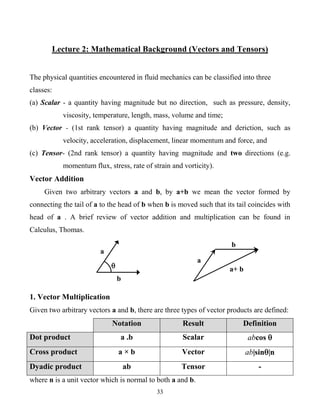
  • 1. 33 Lecture 2: Mathematical Background (Vectors and Tensors) The physical quantities encountered in fluid mechanics can be classified into three classes: (a) Scalar - a quantity having magnitude but no direction, such as pressure, density, viscosity, temperature, length, mass, volume and time; (b) Vector - (1st rank tensor) a quantity having magnitude and deriction, such as velocity, acceleration, displacement, linear momentum and force, and (c) Tensor- (2nd rank tensor) a quantity having magnitude and two directions (e.g. momentum flux, stress, rate of strain and vorticity). Vector Addition Given two arbitrary vectors a and b, by a+b we mean the vector formed by connecting the tail of a to the head of b when b is moved such that its tail coincides with head of a . A brief review of vector addition and multiplication can be found in Calculus, Thomas. 1. Vector Multiplication Given two arbitrary vectors a and b, there are three types of vector products are defined: Notation Result Definition Dot product a .b Scalar abcos  Cross product a × b Vector ab|sin|n Dyadic product ab Tensor - where n is a unit vector which is normal to both a and b. a+ b a b  a b
  • 2. 34 The sense of n is determined from the "right-hand rule". In the above definition, we denote the magnitude (or length) of vector a by the scalar a. Using the following notation: ( ) = scalar = lightface Italic such us a [ ] = vector = boldface Roman such as a { } = tensor = boldface Greek such as  Definition of Dyadic product The word "dyad" comes from Greek: "dy" means two while "ad" means adjacent. Thus the name dyad refers to the way in which this product is denoted: the two vectors are written adjacent to one another with no space or other operator in between. There is no geometrical picture that I can draw which will explain what a dyadic product. It's best to think of the dyadic product as a purely mathematical abstraction having some very useful properties: Dyadic Product ab - that mathematical entity which satisfies the following properties (where a, b, v, and w are any four vectors) 1. ab.v=a(b.v) [which has the direction of a; note that ba.v=b(a.v) which has the dircetion of b]. Thus ab ≠ ba. 2. v.ab=(v.a)b [Thus v.ab ≠ ab.v] 3. ab × v=a(b×v) which is another dyad 4. v×ab=(v×a)b 5. ab:vw=(a.w)(b.v) which is sometimes known as the inner-outer product or the double-out product. 6. a(v+w)=av+aw (distribution for addition) 7. (v+w)a=va+wa 8. (s+t)ab=sab+tab (distribution for scalar multiplication) 9. sab = (sa)b=a(sb)
  • 3. 35 2. Decomposition into Scalar Components (System of Coordinates) A coordinate system in the three-dimensional space is defined by choosing a set of three linearly independent vectors, B={e1, e2, e3}, if none can be expressed as a linear combination of the other two (e.g. i, j, and k). The set B is a basis of the three- dimensional space, i.e., each vector v of this space is uniquely written as a linear combination of this basis: 1 1 2 2 3 3 v v v    v e e e where the vi are called the scalar components of v. In most cases, the vectors e1, e2 and e3 are unit vectors. In the three coordinate systems, i.e., Cartesian, cylindrical and spherical coordinates, the three vectors are, in addition, orthogonal. Hence, in all these systems, the basis B={e1, e2, e3} is orthonormal: 1 . 0 if if        i j ij i j e e i j where ij is called the Kronecker delta. For the cross products of e1, e2 and e3, one gets: 3 1      i j ijk k k e e e where ijk is the permutation symbo or (Levi-Civita), defined as: 1 ,if ijk =123,231,or312 (i.e,an even permutation of 123) 1 ,if ijk = 321,132,or 213 (i.e,an odd permutation of 123) 0 , if any two indices are equal         ijk The Cartesian (or rectangular) system of coordinates (x,y,z), with x , y and z               Its basis is often denoted by {i, j, k} or {ex, ey, ez}. The decomposition of a vector v into (vx, vy, vz) is depicted in figure (1).
  • 4. 36 Figure (1) Cartesian coordinate (x,y,z) The cylindrical and spherical polar coordinates are the two most important orthogonal curvilinear coordinate systems. The cylindrical polar coordinates (r, θ, z),with r 0, 0 2 and z           are shown in fig (2) Figure (2) Cylindrical polar coordinate (r,,z) By invoking simple trigonometric relations, any vector, including those of the bases, can be transformed from one system to another. Table (1) lists the formulas for making coordinate conversions from cylindrical to Cartesian coordinates and vice versa. Table (1) Relations between Cartesian and cylindrical polar coordinates.
  • 5. 37 The spherical polar coordinates (r,,) with r 0, 0 2 and 0 2          together with Cartesian coordinate with the same origin, are in figure (2). Figure (2) Spherical polar coordinate (r,,) The transformation of a vector from spherical to Cartesian coordinates (sharing the same origin) and vice-versa obeys the relations of Table (2). Table (2) Relations between Cartesian and spherical polar coordinates Example. Show that the basis B={er, eθ, ez} of the cylindrical system is orthonormal. Sol. since . . . 1 and . . . 0       i i j j k k i j j k k i , we obtain;         2 2 . cos sin . cos sin cos sin 1 . . . 1 . cos sin . sin cos 0 . .                               r r z z r r z z e e i j i j e e e e k k e e i j i j e e e e
  • 6. 38 H.W. The position vector r defines the position of a point in space, with respect to coordinate system. In Cartesian coordinate, r = x i + y j + z k, show that in cylindrical coordinates, the position vector is given by r = r er + z ez, and in spherical coordinate, r = r er. In the following subsections, we will make use of the vector differential operator nabla (or del), ∇ . In Cartesian coordinates, ∇ is defined by x y z           i j k The gradient of a scalar field f (x, y, z) is a vector field defined by f f f f x y z           i j k The divergence of a vector field v(x, y, z) is a scalar field defined by . y x z v v v x y z           v 3. Tensors In the previous sections, two kinds of products that can be formed with any two unit basis vectors were defined, i.e. the dot product, ei · ej , and the cross product, ei × ej. A third kind of product is the dyadic product, eiej , also referred to as a unit dyad. The unit dyad eiej represents an ordered pair of coordinate directions. The nine possible unit dyads, {e1e1, e1e2, e1e3, e2e1, e2e2, e2e3, e3e1, e3e2, e3e3} A second-order tensor, τ , can thus be written as a linear combination of the unit dyads: 3 3 1 1       ij i j i j e e where the scalars τij are referred to as the components of the tensor τ . Similarly, a third- order tensor can be defined as the linear combination of all possible unit triads eiejek, etc. Scalars can be viewed as zero-order tensors, and vectors as first-order tensors. A tensor, τ , can be represented by means of a square matrix as
  • 7. 39   11 12 13 1 1 2 3 21 22 23 2 31 32 33 3 , , τ                            e e e e e e τ and often simply by the matrix of its components, 11 12 13 21 22 23 31 32 33 τ                    τ Note that the equality sign “=” is loosely used, since τ is a tensor and not a matrix. For a complete description of a tensor by means of matrix, the basis {e1, e2, e3} should be provided. The unit (or identity) tensor, I, is defined by 3 3 1 1 2 2 3 3 1 1         ij i j i j I e e e e e e e e Each diagonal component of the matrix form of I is unity and the non-diagonal components are zero: 1 0 0 0 1 0 0 0 1            I The sum of two tensors, σ and τ , is the tensor whose components are the sums of the corresponding components of the two tensors:   3 3 3 3 3 3 1 1 1 1 1 1                   ij i j ij i j ij ij i j i j i j i j e e e e e e σ τ The product of a tensor, τ , and a scalar, m, is the tensor whose components are equal to the components of τ multiplied by m:   3 3 3 3 1 1 1 1 m m m                   ij i j ij i j i j i j e e e e τ The transpose, τT , of a tensor τ is defined by
  • 8. 40 3 3 1 1      T ji i j i j e e τ The matrix form of τT is obtained by interchanging the rows and columns of the matrix form of τ : 11 21 31 12 22 32 13 23 33 τ                    T τ If τT =τ , i.e., if τ is equal to its transpose, the tensor τ is said to be symmetric. If τT =−τ , the tensor τ is said to be antisymmetric (or skew symmetric). The dyadic product of two vectors a and b can easily be constructed as follows: 3 3 3 3 1 1 1 1 a b ab                      i i j j i j i j i j i j ab e e e e Obviously, ab is a tensor, referred to as dyad or dyadic tensor. Its matrix form is 1 1 1 2 1 3 2 1 2 2 2 3 3 1 3 2 3 3 a b a b a b a b a b a b a b a b a b            ab Note that ab  ba unless ab is symmetric. Given that (ab)T =ba, the dyadic product of a vector by itself, aa, is symmetric. The unit dyads eiej are dyadic tensors, the matrix form of which has only one unitary nonzero entry at the (i, j) position. For example, 2 3 0 0 0 0 0 1 0 0 0            e e The most important operations involving unit dyads are the following:
  • 9. 41 (i) The single-dot product (or tensor product) of two unit dyads is a tensor defined by            i j k l i j k l jk i l e e e e e e e e e e This operation is not commutative (ii) The double-dot product (or scalar product or inner product) of two unit dyads is a scalar defined by;        :       i j k l i l j k il jk e e e e e e e e It is easily seen that this operation is commutative. (iii) The dot product of a unit dyad and a unit vector is a vector defined by          i j k i j k ik i e e e e e e e or          i j k i j k ij k e e e e e e e Obviously, this operation is not commutative. Operations involving tensors are easily performed by expanding the tensors into components with respect to a given basis and using the elementary unit dyad operations. The most important operations involving tensors are summarized below. 1. The single-dot product of two tensors (Tensor product) If σ and τ are tensors, then     3 3 3 3 3 3 3 3 1 1 1 1 1 1 1 1 3 3 3 3 3 3 3 1 1 1 1 1 1 1 3 3 3 1 1 1 k k k                                                                                   ij i j k k ij k i j k i j i j ij k jk i ij j i i j i j ij j i i j e e e e e e e e e e e e e e σ τ σ τ The operation is not commutative. It is easily verified that     I I σ σ σ 2. The double-dot product of two tensors (Scalar product)
  • 10. 42 3 3 1 1 :       ij ij i j i j e e σ τ 3. The dot product of a tensor and a vector (vector product) This is a very useful operation in fluid mechanics. If a is a vector, we have:   3 3 3 3 3 3 1 1 1 1 1 1 3 3 3 3 3 1 1 1 1 1 3 3 1 1 k a a a a a                                                           ij i j k k ij k i j k i j i j k ij k ik k ij j ij i i j k i j ij j i i j a e e e e e e e e a e σ σ Similarly, we find that 3 3 1 1 a                ji j i i j a e σ The vectors σ · a and a · σ are not, in general, equal. 4. Index Notation and Summation Convention So far, we have used three different ways for representing tensors and vectors: (a) the compact symbolic notation, e.g., u for a vector and τ for a tensor; (b) the so-called Gibbs’ notation, e.g., 3 3 3 1 1 1 and u       i i ij i j i i j e e e for u and τ , respectively; and (c) the matrix notation, e.g., 11 12 13 21 22 23 31 32 33 τ                    τ for τ .
  • 11. 43 Very frequently, in the literature, use is made of the index notation and the so- called Einstein’s summation convention, in order to simplify expressions involving vector and tensor operations by omitting the summation symbols. In index notation, a vector v is represented as 3 1 v v     i i i i e v A tensor τ is represented as 3 3 1 1        ij ij i j i j e e τ The nabla operator, for example, is represented as 3 1 i i x x x y z                   i i e i j k where xi is the general Cartesian coordinate taking on the values of x, y and z. The unit tensor I is represented by Kronecker’s delta: 3 3 1 1        ij ij i j i j e e I It is evident that an explicit statement must be made when the tensor τij is to be distinguished from its (i, j) element. With Einstein’s summation convention, if an index appears twice in an expression, then summation is implied with respect to the repeated index, over the range of that index. The number of the free indices, i.e., the indices that appear only once, is the number of directions associated with an expression; it thus determines whether an expression is a scalar, a vector or a tensor. In the following expressions, there are no free indices, and thus these are scalars: 3 1 uv uv      i i i i i u v 3 3 1 1 tr        ii ii i j τ trace for 
  • 12. 44 3 1 3 2 2 2 2 2 2 2 2 2 2 2 2 1 x i i i i u u u u u x x x y z f f f f f f f x x x x x y z                                        y i i z i i i i u or where ∇ 2 is the Laplacian operator to be discussed in more detail in Section (5). In the following expression, there are two sets of double indices, and summation must be performed over both sets: 3 3 1 1 :          ij ji ij ii i j σ τ The following expressions, with one free index, are vectors: 3 3 3 1 1 1 uv uv                   ijk i j ijk i j k k i j e u v 3 1 i f f f f f f x x x y z                   i i i e i j k 3 3 1 1 v v                  ji j ii j i i j e τ v Finally, the following quantities, having two free indices, are tensors: 3 3 1 1 3 3 3 1 1 1 uv uv                        i j i j i j i j ik kj ik kj i j i j k e e uv e e σ τ 3 3 1 1 i i u u x x           j j i j i j e e u Note that ∇ u in the last equation is a dyadic tensor. N.B. Some authors use even simpler expressions for the nabla operator. For example,∇ ・ u is also represented as ∂iui or ui,i ,with a comma to indicate the derivative, and the dyadic ∇ u is represented as ∂iuj or ui,j .
  • 13. 45 5. Differential Operators The nabla operator ∇ , already encountered in previous sections, is a differential operator. In a Cartesian system of coordinates (x1, x2, x3), defined by the orthonormal basis (e1, e2, e3), 3 1 2 3 1 2 3 1 x x x x               i i i e e e e or, in index notation, x     i The nabla operator is a vector operator which acts on scalar, vector, or tensor fields. The result of its action is another field the order of which depends on the type of the operation. In the following, we will first define the various operations of ∇ in Cartesian coordinates, and then discuss their forms in curvilinear coordinates.  The gradient of a differentiable scalar field f, denoted by ∇ f or gradf, is a vector field: 3 3 1 2 3 1 2 3 1 1 f f f f f f x x x x x                           i i i i i i e e e e e  The gradient of a differentiable vector field u is a dyadic tensor field: 3 3 3 3 1 1 1 1 u u x x                           j i j j i j i i i j i i u e e e e if u is the velocity, then ∇ u is called the velocity gradient tensor.  The divergence of a differentiable vector field u, denoted by ∇ · u or div u, is a scalar field 3 3 3 1 2 3 1 2 3 1 1 1 u u u u u x x x x x                                       i i j j ij i i i j i u e e
  • 14. 46 ∇ · u measures changes in magnitude, or flux through a point. If u is the velocity, then ∇ · u measures the rate of volume expansion per unit volume; hence, it is zero for incompressible fluids.  The curl or rotation of a differentiable vector field u, denoted by ∇ ×u or curl u or rot u, is a vector field: 1 2 3 3 3 1 2 3 1 1 1 2 3 u x x x x u u u                               i j j i i j e e e u e e or 3 2 1 3 2 1 1 2 3 2 3 3 1 1 2 u u u u u u x x x x x x                                      u e e e The field ∇ ×u is often called the vorticity (or chirality) of u.  The divergence of a differentiable tensor field τ is a vector field: 3 3 3 3 3 1 1 1 1 1 x x                                 ij k ij i j j k i k i j i j τ e e e e Example. Consider the position vector in Cartesian coordinates, r = x i + y j + z k . For its divergence and curl, we obtain: 3 x y z x y z              r r and 0 x y z x y z            i j k r r
  • 15. 47 Other useful operators involving the nabla operator are the Laplace operator ∇ 2 and the operator u · ∇ , where u is a vector field. The Laplacian of a scalar f with continuous second partial derivatives is defined as the divergence of the gradient: 2 2 2 2 2 2 2 1 2 3 f f f f f x x x             i.e., 2 2 2 2 2 2 2 1 2 3 x x x             For the operator u · ∇ , we obtain:   1 1 2 2 3 3 1 2 3 1 2 3 1 2 3 1 2 3 u u u x x x u u u x x x                               u e e e e e e u The above expressions are valid only for Cartesian coordinate systems. In curvilinear coordinate systems, the basis vectors are not constant and the forms of ∇ are quite different. Notice that gradient always raises the order by one (the gradient of a scalar is a vector, the gradient of a vector is a tensor and so on), while divergence reduces the order of a quantity by one. For any scalar function f with continuous second partial derivatives, the curl of the gradient is zero,   0 f    (1) For any vector function u with continuous second partial derivatives, the divergence of the curl is zero,   0    u (2) Equations (1) and (2) are valid independently of the coordinate system. In fluid mechanics, the vorticity ω of the velocity vector u is defined as the curl of u,     u
  • 16. 48 Example. (a) Express the nabla operator x y z          i j k in cylindrical polar coordinates. (b) Determine ∇ c and ∇ · u, where c is a scalar and u is a vector. (c) Derive the operator u · ∇ and the dyadic product ∇ u in cylindrical polar coordinates. Sol. (a) From Table (1), we have: i = cos θ er − sin θ eθ , j = sin θ er + cos θ eθ and k = ez Therefore, we just need to convert the derivatives with respect to x, y and z into derivatives with respect to r, θ and z. Using the chain rule, we get: sin cos cos sin r x x r x r r y r r z z                                         Substituting now into nabla operator, gives     sin cos cos sin cos sin sin cos r r r r z                                          r r z e e e e e After some simplifications and using the trigonometric identity sin2 θ+sin2 θ =1, we get 1 r r z            r z e e e (b) The gradient of the scalar c is given by; 1 c c c c r r z             r z e e e
  • 17. 49 For the divergence of the vector u, we have;   1 r u u u r r z                        r z r z z u e e e e e e Noting that the only nonzero spatial derivatives of the unit vectors are and            r r e e e e we obtain;     1 1 1 1 1 1 r z r z r z z r u u u u u r r z u u u u u r r r z u u u u r r r z u u ru r r r z                                                                         r r r r r e e u e e e e e u (c)   1 r u u u r r z                        r z z r z u e e e e e e r z u u u r r z            u Finally, for the dyadic product ∇ u, we have;   1 1 1 1 1 1 r r r r u u u r r z u u u r r r u u u u u r r r r r u u u z z z                                                                          r z r z z z r r r r z r z r r z z z r z z z u e e e e e e e e e e e e e e e e e e e e e e e e e e e e
  • 18. 50 1 1 1 r r r u u u r r r u u u u u r r r u u u z z z                                                        z r r r r z z r r z z z r z z z u e e e e e e e e e e e e e e e e e e