Fangbin J A P S2

Modeling of the Sheet-Molding Process for Poly(methyl
methacrylate)

FANGBIN ZHOU,1 SANTOSH K. GUPTAM,2,* AJAY K. RAY1
1
Department of Chemical and Environmental Engineering, National University of Singapore, 10 Kent Ridge Crescent,
Singapore 119260

2
Department of Chemical Engineering, University of Wisconsin, Madison, Wisconsin 53706

Received 3 November 2000; accepted 22 November 2000

ABSTRACT: The sheet-molding process for the production of poly(methyl methacrylate)
(PMMA) involves an isothermal batch reactor followed by polymerization in a mold (the
latter is referred to as a “sheet reactor”). The temperature at the outer walls of the mold
varies with time. In addition, due to finite rates of heat transfer in the viscous reaction
mass, spatial temperature gradients are present inside the mold. Further, the volume
of the reaction mass also decreases with polymerization. These several physicochemical
phenomena are incorporated into the model developed for this process. It was found
that the monomer conversion attains high values of near-unity in most of the inner
region in the mold. This is because of the high temperatures there, since the heat
generated due to the exothermicity of the polymerization cannot be removed fast
enough. However, the temperature of the mold walls has to be increased in the later
stages of polymerization so that the material near the outer edges can also attain high
conversions of about 98%. This would give PMMA sheets having excellent mechanical
strength. The effects of important operating (decision) variables were studied and it
was observed that the heat-transfer resistance in the mold influences the spatial
distribution of the temperature, which, in turn, influences the various properties (e.g.,
monomer conversion, number-average molecular weight, and polydispersity index) of
the product significantly. © 2001 John Wiley & Sons, Inc. J Appl Polym Sci 81: 1951–1971, 2001

Key words: poly(methyl methacrylate); sheet-reactor; sheet-molding; modeling; poly-
mer reactor

INTRODUCTION ried out for several decades,1 more art than sci-
ence is involved in this operation. Very little work
Poly(methyl methacrylate) (PMMA) is a major has been reported in the open literature on the
commodity plastic. An important application of modeling and simulation of this process. In the
PMMA stems from its transparency, and it is last two decades, a considerable amount of knowl-
used as a replacement of glass. Even though edge has become available on the modeling of the
large-scale sheet molding of PMMA has been car- bulk polymerization of methyl methacrylate
(MMA). In this article, this knowledge is extended
to model the industrial process of the sheet mold-
Correspondence to: A. K. Ray (cheakr@nus.edu.sg). ing of PMMA.
*On leave from the Indian Institute of Technology, Kan- A distinguishing feature of the bulk polymer-
pur, 208016, India.
Journal of Applied Polymer Science, Vol. 81, 1951–1971 (2001)
ization of MMA is the presence of an extremely
© 2001 John Wiley & Sons, Inc. strong Trommsdorff2,3 effect. This is a manifesta-

1951

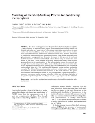
1952 ZHOU, GUPTAM, AND RAY

Table I Kinetic Scheme for Bulk-addition tion of the significant decrease of the apparent
Polymerization of MMA rate constants (see Table I), kt and kp, as well as
the initiator efficiency, f, at monomer conversions
f kd
above about 40%. This is because the viscosity of
Initiation I O 2R
¡
ki
the reaction mass increases significantly and dif-
R M ¡ P1 fusional limitations assume considerable signifi-
kp cance under these conditions. Excellent models4 –7
Propagation Pn M O Pn
¡ 1 for this effect have appeared in the last few years
kt and have been reviewed recently.8,9 These can
Termination Pn Pm ¡ Dn Dm now be applied to simulate large-scale operations
(disproportionation)
where physicochemical effects like heat and mass
transfer are involved, in addition to chemical re-

Figure 1 Schematic diagram of the sheet-molding process for PMMA: (a) batch
reactor; (b) mold (sheet reactor), with a repeating computational shell having a volume
V*out ALx,ini; (c) wall-temperature history in the sheet reactor commonly used in
industry.1

MODELING OF SHEET-MOLDING PROCESS FOR PMMA 1953

Table II Equations for the Batch Reactor mer conversion and of the average molecular
weights of the polymer during this process.
dI*
kd I*
dt
dM* *M*
0 R*M* FORMULATION
kp ki
dt V* V*
dR* R*M* The sheet-molding process for PMMA as de-
2fk dI* k i scribed above is now modeled. The process, shown
dt V*
d *0 R*M* * *
0 0
schematically in Figure 1, involves two reactors,
ki kt namely, a batch reactor followed by a “sheet” re-
dt V* V*
d * 1 R*M* *M*
0 * *
0 1
actor. The polymerization in the isothermal batch
ki kp kt reactor was modeled and extensively studied ear-
dt V* V* V*
d * 2 R*M* * 2 *
0 1 * *
0 2
lier.7,10 –13 Table II summarizes the mass balance
ki k pM* kt and moment equations describing this reactor.
dt V* V* V*
d * *2 The change in the volume during polymerization
0 0
kt
dt V*
d * 1 * *
0 1
kt Table III Cage, Gel, and Glass-effect Equations
dt V* for Bulk Polymerizations7
d * 2 * *
0 2
kt
dt V* 1 1 M 1
P* M * M* MWm 1 f T (1)
0 f f0 V exp I3 ref

1 1 0 1
Initial conditions (I.C.); t* 0: choose V * arbitrarily. I*
0 T 2
(2)
t n
I*0 [I 0 ]*V * ; M*
0 M* 0
* *
m (T 0 )V 0 /(MWm ); R*,
* ,
k,0
kt k t,0 V exp ref
* (k 0, 1, 2) 0.
k,0 1 1 0 1
p T (3)
kp k p,0 V exp 13 ref
action. The sheet molding of PMMA is an example ˆm
m m V*
which is modeled in this work. p p
ˆp
V*
In this process (see Fig. 1), a volume, V *, of a
0
13
(4)
ˆm
V * V fm ˆp
V *V fp
mixture of M * mol of MMA and I * mol of the
0 0
m m p p

initiator (AIBN) is first polymerized in a well-
(5)
stirred, isothermal (T *) batch reactor. A volume,
0
ref
Vfp
T * , of the product prepolymer is obtained. The
out M* MWm P*
monomer conversion in the batch reactor is x * V batch ; (6)
m,out, m T*
0 p T*0
and the total reaction time is T * . This mixture is
out Vj,new t in Table V sheet
then filled into the mold. The latter is a thin
hollow box, the faces of which are formed of two M* MWm / m T *
0
large parallel glass sheets (each of area Amold), m batch ; (7)
M* MWm M* M* MWm
0
separated by a distance of 2Lx,ini by the use of thin m T*
0 p T*0
strips of compressible material (spacers). Further
m,j,new t in Table V sheet
polymerization of the reaction mass takes place in 1 (8)
p m
the completely filled mold as it passes through a ˆm
V * MWm
temperature-programmed oven. The tempera- (9)
13 ˆp
V*Mjp
ture, Tw(t), of the outer surfaces of the reaction
mass is assumed to be a function of time, t. Beat- Î
V* MWI
tie1 gave the typical temperature history used in I3 ˆp (10)
V*Mjp
industry [Fig. 1(c)]. The elastic spacers become kd 0
k dexp Ed /Rg T (11)
compressed as polymerization takes place in the 0
k p,0 k p,0exp Ep /Rg T (12)
mold, to accommodate the contraction in the vol-
0
ume of the reaction mixture. A computer model is k t,0 k exp
t,0 Et /Rg T (13)
first developed for the polymerization of MMA in
Variables with a superscript * are used for the batch reac-
the mold, to study the effect of the nonisothermal tor; variables with subscript j are used for the sheet reactor ( j
temperature history on the variation of the mono- 1, 2, . . . , N).


Table IV Parameters Used for Bulk Polymerization of MMA
with AIBN7,14 –16

m 966.5 1.1[T(K) 273.15] kg/m3
p 1200 kg/m3
f0 0.58
0
kd 1.053 10 15 s 1
0
k p,0 4.917 10 2 m3 mol 1 s 1
0
k t,0 9.8 10 4 m3 mol 1 s 1
ki kp
Ed 128.45 kJ/mol
Ep 18.22 kJ/mol
Et 2.937 kJ/mol
(MWm ) 0.10013 kg/mol
(MWI ) 0.06800 kg/mol
Parameters for the cage, gel, and glass effects7

ˆ
V* 9.13 10 4 m3/kg
I
ˆ
V* 8.22 10 4 m3/kg
m
ˆ
V* 7.70 10 4 m3/kg
p
M jp 0.18781 kg/mol
1
4
V fm 0.149 2.9 10 [T(K) 273.15]
4
V fp 0.0194 1.3 10 [T(K) 273.15 105]
7
Correlations used for the ’s

log10[ t (T), s] a1 a 2 (1/T) a 3 (1/T 2 )
log10[ p (T), s] b1 b 2 (1/T) b 3 (1/T 2 )
log10[10 3 f (T), m3 mol 1] c1 c 2 (1/T) c 3 (1/T 2 )
2 5
a 1 1.2408 10 ; a 2 1.0314 10 ; a 3 2.2735 10 7
b 1 8.0300 10 1; b 2 7.5000 10 4; b 3 1.7650 10 7
c 1 2.0160 10 2; c 2 1.4550 10 5; c 3 2.7000 10 7
Parameters for the sheet reactor14–16

C p,mix 1.674 kJ kg 1 K 1
Hr 58.19 kJ/mol
KT 0.13 W m 1 K 1
Mj,new t MWm Pj,new t
mix,j t
Vj,new t
A V * /L x,ini; (independent of time)
out
V*out 0.0065 m3

is accounted for, since the volume, V*, at any presence of diffusional limitations, while Table IV
time, t*, is computed as the sum of the volumes of gives the values of all the parameters used. These
the unreacted monomer present and that of the tables provide the same information as given by
polymer produced until that time. A new variable, Seth and Gupta7 and so the details are not re-
P*(t*), is deﬁned in this table. This is the total peated here. These stiff ordinary differential
mass (kg) of the polymer produced until time t* in equations17 (ODEs) are integrated from t* 0,
the batch reactor. Tracking of this variable in the using the subroutine DIVPAG, in the IMSL li-
sheet reactor (described later) makes it easy to brary, for the given conditions (T *, V*, and [I0]*
0 0
evaluate the local values of the monomer conver- etc.; M * being computed from V * and T *). The
0 0 0
sion. Table III presents the equations for the rate value of the parameter, TOL, used in the code
constants and the initiator efﬁciency, f, in the DIVPAG was 10 6. The integration is continued


Table V Equations for the Sheet Reactor, t Table V Continued
< time < t t
Integrate PDEs after converting to ODE–IVPs using
PDEs DSS002, from t to t t, to give
Ij t t ; Mj t t ; Rj t t ; k,j t t ;
I
kd I k 0, 1, 2 ;
t
k,j t t ; k 0, 1, 2 ; T j t t ;
M Then:
A x kp M 0 ki MR
t Pj t t Pj t Mj t Mj t t MWm
R Mj t t MWm Pj t t
A x 2fk dI A x k iRM Vj t t
t m Tj t t p Tj t t
0
xj t t Vj t t /A
2
A x k iRM kt 0
t N

Lx t t xj t t
1
A x k iRM k p 0M kt 0 1 j 1
t
Redistribute grid planes instantaneously at t t:
A x
2
k iRM k pM 2 kt x j,new t t Lx t t /N
0 1 0 2
t ● Plot
0 2
A x kt 0 Ij t t /V j t t ; Mj t t /V j t t ;
t
Rj t t /V j t t ; k,j t t /V j t t ;
1
A x kt 0 1 k,j t t /V j t t ; Tj t t ;
t
Pj t t /V j t t ;
2
A x kt 0 2
t as functions of x (center points of each ﬁnite-
2
T kp M 0 difference cell to be used for plotting value for j th
mix Cp,mixT KT Hr
t x2 A x 2 cell); see Figure A
● Connect by smooth curves
“Initial” conditions at time t (after redistribution of ● Read off values on smooth curves at equispaced
grid planes in the previous time interval); j 1, locations, x j,new:
2, . . . , N, at time t; known (from previous Lx t t 2j 1
computation): x j,new t t ;
N 2
I j,new t ; Mj,new t ; Rj,new t ; k,j,new t , k,j,new t ;
j 0, 1, . . . N 1 See Fig. A
k 0, 1, 2 ● Multiply all the interpolated concentrations (not
T j,new t ; Pj,new t ; the temperature) by appropriate V j,new(t t)
x j,new t Lx t /N; Vj,new t A xj,new t A x j,new(t t)
● Gives: T j,new(t t) as well as I j,new(t t);
Mj,new t MWm M j,new(t t); R j,new(t t); k,j,new(t t);
m,j,new t Vj,new t
m Tj,new t (k 0, 1, 2); k,j,new(t t); (k 0, 1, 2);
(Special case; at t 0, use all moles as (1/N) P j,new(t t)
(output value from batch reactor) and all T j as T * ).
0

Boundary conditions (BCs):

at x 0 center : until the monomer conversion reaches the desired
T value, x * , at which time t*
out T * This code
out
0 provides the composition and volume of the pre-
x
at x Lx t wall : polymer that is fed into the mold.
The prepolymer is poured into the mold at time
0 t 20 h, Twall 55°C
T * . We redeﬁne the time, t (all the variables in
out
20 h t 24 h, Twall 55 7.5 t 20 °C the sheet reactor are used without the superscript
24 h t 27 h, Twall 85°C *), in this reactor, to start from t 0. Thus, t 0
27 h t 28 h, Twall 85 20 t 27 °C in this sheet reactor is identical to t* T * in the
out
28 h t 36 h, Twall 65°C batch reactor. The initial thickness of the mold is
2Lx,ini. The symmetry of the sheet reactor is now


Table VI Equations for Monomer Conversion,
Average Molecular Weights, and PDI

Batch reactor

At any time, t*; 0 t* t*
out
x*
m M * M* /M *
0 0

*
1 *
1
M* n MWm * *
0 0

*
2 *
2
M*
w MWm * *
1 1

M*w
PDI*
M*n

Sheet reactor

At time t; 0 t t f ; [values after redistribution of
grid planes]
Local values:
Pj,new t t
M**
0, j M j,new t t
MWm
Figure 2 Finite-difference grid planes in the repeat- Mj,new t t
xm,j,new t t 1
ing computational shell in the sheet reactor. M* 0,j
1 1 j,new t t
Mn,j,new t t
0 0 j,new t t
exploited. It is assumed that the volume, V * , of
out 2 2 j,new t t
Mw,j,new t t
the prepolymer from the batch reactor ﬁlls only a 1 1 j,new t t
(repeating) part of the mold, shown as the shaded Mw,j,new t t
PDIj,new t t
region in Figure 1(b). This corresponds to a cross- Mn,j,new t t
sectional area, A ( Amold), of each glass plate. In Cross-section average values:
fact, the volume, V *, of the initial mixture taken
0
N

in the batch reactor can be selected somewhat M*
0 Mj,new t t
j 1
arbitrarily, and the area, A, of the sheet reactor x m,new t t
corresponding to the associated prepolymer (of M*
0
N

1 1 j,new t t
j 1
Mn,new t t MWm
N

0 0 j,new t t
j 1
N

2 2 j,new t t
j 1
Mw,new t t MWm
N

1 1 j,new t t
j 1

Mw,new t t
PDInew t t
Mn,new t t

volume V * ) can be computed. This area, A, forms
out
a repeating “computational cell” (of volume ALx,ini
Figure A Interpolation procedure (example of M/V). V * ). What occurs in one such computational
out


Figure 3 Section-average values of xm, Mn, and PDI, and half the sheet thickness, Lx,
as a function of time, t, for the reference conditions . Solid lines represent the batch
reactor while dotted lines represent the sheet reactor.

cell is duplicated in other similar cells in the mold tions (complete symmetry in these two directions
(assuming that the end effects are negligible). is assumed). The equations describing the poly-
Thus, the solution for a single computational cell merization in the computational cell are, there-
gives information about the entire mold. This fore, partial differential equations (PDEs).
computational repeating cell is somewhat akin to The PDEs describing the polymerization in a
a unit cell in a crystal. computational cell in the sheet reactor are of the
Equations representing the mass balance, mo- following form (see Table V):
ments, and energy balance for the repeating com-
2
putational cell in the sheet reactor can easily be x/ t f x, x/ x2, u (1a)
written. These equations must account for the
heat transfer through the viscous reaction mass xi t 0 x* ; i
i,out 1, 2, . . . , 9; x10 t 0 T*0
in the transverse (x) direction. The temperature, (1b)
T, as well as the concentrations of all species and
moments in this cell would be functions of both T x Lx t Tw t (1c)
the time, t, as well as the location, x. No variation
is expected for any variable in the y- and z-direc- T/ y x 0 0 (1d)


Figure 4 Variation of the local values of the temperature (T), xm, Mn, and PDI in the
sheet reactor, as a function of x at different times. x 0 represents the center plane in
the mold. Values of the decision variables are those for the reference case . The
temperature profiles for t 20 h are the same as in Figure 6(a) [Tw(t) being the same
for these two cases for these values of t].

In eq. (1), x is the vector of state variables, xi, An additional complication present in the
defined by present problem is that the thickness, Lx, of the
computational cell decreases with time. This
T
x I, M, R, 0 , 1 , 2 , 0 , 1 , 2 ,T (2) makes this into what is referred to as the moving
boundary problem. To obtain solutions to this
and u is the vector of independent operating (or problem, we simplify it and assume that the en-
decision) variables, ui. The following is the set of tire contents of any computational cell at time t
decision or control variables in this problem: 0 and having an initial volume of AL,ini remain
inside the cell of volume ALx (having the same
u T*, I0 *, x* , Lx,ini, Tw t
0 out
T
(3) cross-sectional area, A) as the cell becomes thin-
ner with time.
These variables can easily be changed in an ex- The PDEs in eq. (1) and Table V can be solved
perimental/industrial system and so comprise a using the method of lines (finite differenc-
reasonable set to use. These variables have to be es).17,18 This technique is used to convert the
specified (“givens” of the problem) so as to be able PDEs into a coupled set of several ODE–IVPs
to evaluate the evolution of the state variables using the DSS002 code,18 and the subroutine
over time. In addition, these variables could be DIVPAG is then used to integrate the equa-
used in future optimization studies. tions. The details of the numerical procedure


Figure 5 xm, Mn, PDI, and Lx as a function of t in the two reactors when Tw(t) is
constant at 55oC. Solid lines represent the batch reactor while dotted lines represent
the sheet reactor.

used are now described: The domain, 0 x Lx, ing of the grid planes would become unequal at
at any time, t, is divided into N 1 equispaced time t t, as polymerization progresses. Fol-
finite-difference grid planes (N cells of equal lowing the polymerization in cells having differ-
volume), as shown in Figure 2. The region be- ent thicknesses would lead to severe computa-
tween two consecutive grid planes, and having a tional problems. Hence, at the end of each in-
cross-sectional area, A, is referred to as a finite- terval of time, we redistribute the N 1 grid
difference “cell.” The reaction mixture in each planes using an interpolation scheme (see Fig.
finite-difference cell is assumed to polymerize A). The domain, 0 x Lx(t t) is redivided
during the short interval of time, t t t t, at time t t, into N 1 new, equispaced grid
at a temperature that is assumed to remain planes. Obviously, the average values of T and
constant at the instantaneous local value, T(x, of the concentrations and moments at (the cen-
t), for this short period. The volume of each ter of each) finite-difference cell would change
finite-difference cell is, similarly, assumed to during this instantaneous operation of redistri-
remain constant during this short interval of bution of the grid planes. The detailed proce-
time and is (re-)computed at the end of the dure and equations for estimating the new in-
interval for each cell. Since the contraction of terpolated values of all the variables during the
the volume would differ for each cell, the spac- redistribution are described in Table V.


Figure 6 Variation of the local values of T, xm, Mn, and PDI with x at different values
of t. Tw(t) constant at 55oC. T(x) does not change any further for t 9.278 h.

The entire set of coupled equations for each mer in cell j is, thus, simply the sum of Mj and
finite-difference cell are solved along with the Pj/(MWm). The monomer conversion in cell j is
equations in Table III for t t t t. There- written as 1 Mj /[Mj (Pj /(MWm)]. In this study,
after, interpolation is carried out to obtain the the value of N was taken as 8, and it was con-
new values of all the variables after the instanta- firmed that almost identical results were ob-
neous redistribution of the grid planes. This pro- tained when higher values of N (20, 30, or 40)
cedure is repeated until the end of the sheet- were used.
casting process, t tf. At every interval, the sec-
tion-average values of the monomer conversion
(xm) and of the average molecular weights (Mn RESULTS AND DISCUSSION
and Mw) are evaluated using the expressions
given in Table VI. The calculation of the local
A computer code for the simulation of the entire
value of the monomer conversion (conversion in
process was written in FORTRAN 90 and tested
any finite-difference cell) is slightly difficult since
extensively for errors. The code was then used to
we are unable to “define” an appropriate value of
generate results for the following “reference” (ref)
the “initial” moles of monomer in cell j because of
conditions of the decision variables :
the continuous redistribution of the grid planes.
This is why we introduce a new variable, Pj, and
keep updating it as the cell transforms due to the T*
0 55°C
redistribution and interpolation procedures. Pj I0 * 22.0 mol/m3
represents the mass of the polymer in cell j at any
time. The “initial” number of moles of the mono- x*
out 0.7


Figure 7 xm, Mn, PDI and Lx as a function of t in the two reactors. T *
0 65°C. All
other decision variables are at their reference values.

L x,ini 0.0065 m Figure 4 shows the spatial variation of the local
values of the temperature, monomer conversion,
T w t : Table V (4) Mn, and PDI at different times in the sheet reac-
tor. The variations of these variables, when the
The CPU time taken on an SGI Origin 2000 su- wall temperature in the sheet reactor is kept con-
percomputer for one such simulation run was stant at 55°C all through the operation, are
600 s. shown for comparison in Figures 5 and 6. The
Figure 3 shows the variations of the section- average conversion in the nonisothermal case is
average values of the monomer conversion, xm, observed to be only very slightly larger, and the
the number-average molecular weight, Mn, and average molecular weight, slightly lower, near
the polydispersity index, PDI, as a function of the end of the operation, after the wall tempera-
time, t, for the reference conditions given in eq. ture increases (after about 24 h). This is expected
(4). The solid curve represents the operation of physically, since the increase of the temperature
the isothermal batch reactor at 55°C, while the near the end of the operation reduces the differ-
dashed curve represents the sheet reactor under ence between the polymerization and the glass
nonisothermal conditions. The variation of (half) transition temperatures (overcomes the glass ef-
the sheet thickness, Lx, with time is also shown. fect to some extent) and so enables further poly-


Figure 8 Local values of T, xm, Mn, and PDI as a function of x at different values of
t. T * 65°C. All other decision variables are at their reference values.
0

merization in the reference case. It is observed molecular weights for the sheet reactor at differ-
that the sheet thickness is smaller under noniso- ent locations and times, both for the nonisother-
thermal conditions because of this additional po- mal and the constant wall-temperature cases
lymerization. (Figs. 4 and 6). Even though there is no signiﬁ-
An interesting phenomenon is observed when cant difference between the results for these two
we compare the plots for the local values of the cases for Mn, it is found that the monomer conver-
monomer conversion and the number-average sion increases dramatically in the outer (oven-side)


Figure 9 xm, Mn, PDI and Lx as a function of t in the two reactors. [I0]* 15 mol/m3.
All other decision variables are at their reference values.

region of the sheet from about 91 to about 97.5% in there. Figures 4(d) and 6(d) show that the local
the case of nonisothermal operation. This, in fact, values of PDI in the PMMA sheet are slightly lower
suggests why one uses temperature programming in the nonisothermal case than when the operation
in this process. The exothermic nature of the poly- is isothermal. This is again because of higher con-
merization leads to high temperatures (approxi- versions in the nonisothermal case. In this case, too,
ately 150°C) near the center of the sheet during the as in the case of the average monomer conversion,
early period of polymerization [Fig. 6(a); same T(x)
the average value of the polydispersity index (PDI)
for t 20 h for both isothermal and nonisothermal
does not display any dramatic differences. Clearly,
cases]. This leads to monomer conversions near
one has to study local rather than section-average
unity in the central region (core). In contrast, the
material near the wall experiences lower tempera- values to understand reactor behavior. This insight
tures in the isothermal case, and so the monomer can be of immense use in formulating appropriate
conversion in that region does not go above about optimization problems for this process in the future.
91%. The introduction of higher wall temperatures The effects of a few of the more important op-
in the later stages of polymerization remedies this erating (decision) variables from among those
[see Fig. 4(a)] and leads to the formation of PMMA listed in eq. (4), are now studied (other results can
sheets that are stronger at the outer regions due to be supplied on request). These results can be com-
the attainment of higher monomer conversions pared with the reference results shown in Figures


t. [I0]* 15 mol/m3. All other decision variables are at their reference values.

3 and 4. Figures 7 and 8 show the effect of chang- average value of the number-average molecular
ing the temperature, T *. This is the temperature
0 weight. The section-average value of the PDI is
of the isothermal batch reactor, as well as the higher. These effects of temperature are expected
wall temperature for the ﬁrst 20 h in the sheet for PMMA systems.
reactor and so is an important decision variable. Figures 9 and 10 show the effect of a decrease
Higher values of T * speed up the reaction, but
0 in the initiator concentration, [I0]*, in the feed to
also lead to a signiﬁcant lowering of the section- the batch reactor from the reference value of 22 to


Figure 11 xm, Mn, PDI and Lx as a function of t in the two reactors. L,ini 0.01 m. All

15 mol/m3. It is clear that lower values of the its section-average value). The percent shrinkage
initiator concentration lead to higher spatial-av- is almost the same in both these cases (8.6% for
erage values of Mn. This is expected physically, L,ini 0.01 m compared to 8.4% for the reference
since lower initiator concentrations lead to lower case).
concentrations of free radicals in the reaction Figures 13 and 14 show the effect of changing
mass and reduce the probability of termination. A Tw(t), the wall-temperature history. Only one pa-
similar effect is observed in Figure 10(c) which rameter characterizing the function, Tw(t), is
shows the variation of the local values of Mn. changed—the highest temperature, Tw,max, from
Figure 10 shows the variation of the local values 85 to 90°C during 24 h t 27 h. Obviously, the
of the monomer conversion and the PDI in the rate of increase or decrease of Tw(t) during 20 h
mold. The effects of the initiator concentration on t 24 h and 27 h t 28 h (Table V) are
these are small. higher. The most important inﬂuence of this is
Figures 11 and 12 show the effect of increasing that higher local values of the monomer conver-
(half) the initial sheet thickness, L,ini. As L,ini is sion are achieved near the walls.
increased, the heat-transfer resistance increases Figures 15 and 16 show the effect of reducing
and temperatures in the inner core (at interme- x * , the monomer conversion at the end of the
out
diate values of t) become higher, leading to higher batch reactor, to 0.3. The Trommsdorff effect is
values of the local monomer conversion (as well as manifested almost entirely inside the mold in this


t. L,ini 0.01 m. All other decision variables are at their reference values.

case (in the reference case, where x * was 0.7,
out obtained. Interestingly, the section-average value
part of this effect occurred in the batch reactor). of the number-average molecular weight is
The temperature history experienced by the reac- slightly higher, but the section-average value of
tion mass is obviously different in this case, and the PDI is much lower in this case. These would
because of this, higher values of the local and have considerable inﬂuence on the properties of
section-average values of the monomer conver- the ﬁnal product. This is an interesting inference
sion (and, so, slightly thinner PMMA sheets) are and can be useful in optimization studies as well.


Figure 13 xm, Mn, PDI and Lx as a function of t in the two reactors. Tw,max 90°C
during 24 h t 27 h in the sheet reactor. All other decision variables are at their
reference values.

CONCLUSIONS Cp,mix specific heat of the reaction mix-
ture in the sheet reactor (J
kg 1 K 1)
A model was developed for the sheet molding of
MMA. Some interesting observations were made Dn dead polymer molecule having n
regarding the influence of temperature program- repeat units
ming in the furnace on the local values of the mono- Ed, Ep, Et activation energies for the reac-
mer conversion in a thin region near the walls of the tions in Table I (kJ/mol)
mold. The insights developed herein could be useful f initiator efficiency
in optimization studies of this operation. f0 Initiator efficiency in the limit-
ing case of zero diffusional re-
sistance
NOMENCLATURE Hr enthalpy of the propagation re-
action (J/mol)
A cross-sectional area of the sheet I* moles of initiator in the batch
reactor (m2) reactor at any time, t (mol)


t. Tw,max 90°C during 24 h t 27 h in the sheet reactor. All other decision variables
are at their reference values.

[I0]* molar concentration of initiator in M*
0 “initial” moles of monomer corre-
feed of batch reactor (mol/m3) sponding to cell, j, in the sheet
Ij moles of initiator in any cell, j, in reactor after regridding, at
the sheet reactor at time t (mol) time t (mol)
kd, ki, kp, kt rate constants for initiation, Mj moles of monomer in cell, j, in
propagation, and termination the sheet reactor at time t
in the presence of the gel and (mol)
glass effects (1/s, or m3 mol 1 Mjp molecular weight of the polymer
s 1) jumping unit (kg/mol)
ki,0, kp,0, kt,0 intrinsic (in absence of cage, gel, Mn,j number-average molecular
and glass effects) rate con- weight [ (MWm) ( 1 1)/( 0
stants (m3 mol 1 s 1) 0)]j in cell, j, in the sheet
k0 , kp,0, kt,0
d
0 0
frequency factors for intrinsic reactor at time t (kg/mol)
rate constants (1/s or m3 mol 1 Mw,j weight-average molecular weight
s 1) [ (MWm) ( 2 2)/( 1 1)]j
KT thermal conductivity of the reac- in cell, j, in the sheet reactor at
tion mixture in the ﬁlm reac- time t (kg/mol)
tor (W m 1 K 1) (MWI), (MWm) molecular weights of pure pri-
Lx half the sheet thickness at time t mary radicals and monomer
(m) (kg/mol)
M* moles of monomer in the batch N number of cells in the sheet re-
reactor at time t (mol) actor


Figure 15 xm, Mn, PDI and Lx as a function of t in the two reactors. x *
out 0.3. All

Pn growing polymer radical having t time interval (s)
n repeat units T temperature of the reaction mix-
Pj mass of polymer in cell, j, in the ture in cell, j, in the sheet re-
sheet reactor at time t (kg) actor at time t (K)
PDIj polydispersity index in cell, j, in T* temperature of the isothermal
the sheet reactor at time t batch reactor (K)
R* moles of primary radicals in the V* volume of reaction mixture in
batch reactor at time t*(mol) the batch reactor at time
Rj moles of primary radicals in cell, t*(m3)
j, in the sheet reactor at time t Vj volume of reaction mixture in cell, j,
(mol) in the sheet reactor at time t (m3)
Rg universal gas constant (kJ mol 1 Vfm, Vfp free volume of monomer and
K 1) polymer
t reaction time in the batch reac- ˆ ˆ ˆ
V *, V * V * speciﬁc critical hole free volumes
I m, p
tor (h) of initiator, monomer, and
t reaction time in the sheet reac- polymer (m3/kg)
tor [t 0 at start of polymer- x transverse location in the sheet re-
ization in the mold] (h) actor from the center line (m)


t. x *
out 0.3. All other decision variables are at their reference values.

xj thickness of cell, j, in the sheet Greek Letters
reactor at time t (m)
x*
m monomer conversion in the overlap factor
batch reactor at time t* 13, I3 ratio of the molar volume of the monomer
xm,j local monomer conversion in and initiator jumping unit to the criti-
cell, j, in the sheet reactor at cal molar volume of the polymer, re-
time t spectively


f, p, t parameters in the model for the cage, REFERENCES
gel, and glass effects, respectively
(m3/mol, s, s)
* 1. Beattie, J. O. Mod Plast 1969, 46, 684.
k kth (k 0, 1, 2, . . .) moment of live
2. Trommsdorff, V. E.; Kohle, H.; Lagally, P. Makro-
polymer radicals, Pn, in the batch re-
mol Chem 1947, 1, 169.
actor at time t* (mol) 3. Norrish, R. G. W.; Smith, R. R. Nature 1942, 150,
* kth (k 0, 1, 2, . . .) moment of dead
k 336.
polymer radicals, Dn, in the batch re- 4. Chiu, W. Y.; Carratt, G. M.; Soong, D. S. Macromol-
actor at time t* (mol) ecules 1983, 16, 348.
k,j kth (k 0, 1, 2, . . .) moment of live 5. Achilias, D. S.; Kiparissides, C. J Appl Polym Sci
polymer radicals, Pn, in cell, j, in the 1988, 35, 1303.
sheet reactor at time t (mol) 6. Achilias, D. S.; Kiparissides, C. Macromolecules
k,j kth (k 0, 1, 2, . . .) moment of dead 1992, 25, 3739.
polymer radicals, Dn, in cell, j, in the 7. Seth, V.; Gupta, S. K. J Polym Eng 1995, 15, 283.
sheet reactor at time t (mol) 8. Gao, J.; Penlidis, A. J Macromol Sci-Rev Macromol
n number-average chain length Chem Phys 1996, 36, 199.
9. Mankar, R. B.; Saraf, D. N.; Gupta, S. K. Ind Eng
m, p densities of pure (liquid) monomer and
of pure polymer [functions of temper- Chem Res 1998, 37, 2436.
ature only] (kg/m3) 10. Zhou, F. B.; Gupta, S. K.; Ray, A. K. J Appl Polym
Sci 2000, 78, 1439.
m, p volume fractions of monomer and poly-
11. Chakravarthy, S. S. S.; Saraf, D. N.; Gupta, S. K.
mer in the reaction mass
J Appl Polym Sci 1997, 63, 529.
Subscripts/Superscripts 12. Garg, S.; Gupta, S. K. Macromol Theory Simul
1999, 8, 46.
13. Ray, A. B.; Saraf, D. N.; Gupta, S. K. Polym Eng Sci
ini starting value in the sheet reactor
1995, 35, 1290.
f ﬁnal value (at t tf) at the end of the sheet 14. Vargaftik, N. B. Handbook of Thermal Conductiv-
reactor ity of Liquids and Gases; CRC: Boca Raton, FL,
new values after instantaneous redistribution 1994.
of the grid planes in the sheet reactor 15. H. F.; Mark, Bikales, N. M.; Overberger, C. G.;
0 feed to the batch reactor Menges, G. Encyclopedia of Polymer Science Engi-
out product of the batch reactor neering, 2nd ed.; Wiley: New York, 1986; Vol. 4.
w wall of the sheet reactor 16. Louie, B. M.; Soong, D. S. J Appl Polym Sci 1985,
* values in the batch reactor 30, 3707.
17. Gupta, S. K. Numerical Methods for Engineers;
Symbols New Age International: New Delhi, 1995.
. . .cross-section average (over 0 x Lx) in 18. Schiesser, W. E. The Numerical Method of Lines;
the sheet reactor at time t Academic: New York, 1991.

Fangbin J A P S2

Recomendados

Recomendados

Más contenido relacionado

Destacado

Destacado (7)

Similar a Fangbin J A P S2

Similar a Fangbin J A P S2 (20)

Más de Yose Rizal

Más de Yose Rizal (19)

Último

Último (20)

Fangbin J A P S2