All of material inside is un-licence, kindly use it for educational only but please do not to commercialize it. Based on 'ilman nafi'an, hopefully this file beneficially for you. Thank you.

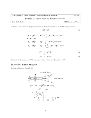
1. Z
Z
Z
2.092/2.093 — Finite Element Analysis of Solids & Fluids I Fall ‘09
Lecture 6 -Finite Element Solution Process
Prof. K. J. Bathe MIT OpenCourseWare
In the last lecture, we used the principle of virtual displacements to obtain the following equations: KU = R (1)
K =Σ K(m) ; K(m) = B(m)T C(m)B(m)dV (m)
mV (m) R = RB + RS
RB =Σ RB (m) ; RB (m) = H(m)T fB(m)dV (m) mV (m)
ff mS Si i(m) f S
RS =Σ R(m) ; R(m) =Σ HSi(m) T fSi(m) dSi(m)
f
u(m) = H(m)U (2)
↓
ε(m) = B(m)U (3) Note that the dimension of u(m) is in general not the same as the dimension of ε(m).
Example: Static Analysis
Reading assignment: Example 4.5
1

2. | {z } | {z }
Lecture 6 Finite Element Solution Process 2.092/2.093, Fall ‘09
Assume:
i. Plane sections remain plane
ii. Static analysis no vibrations/no transient response
→
iii. One-dimensional problem; hence, only one degree of freedom per node Elements 1 and 2 are compatible because they use the same U2. Next, use a linear interpolation function.
⎡
(1)(x)= xx ⎣u1 − 100 100 0
H(1)
⎡
11ε(1)(x)= | − 100 {z100 0 } ⎣
B(1)
⎡⎤
1 Z 100 ⎢ − 100 ⎥h K = E 1 ⎢ 1 ⎥ 11
·· ⎣ 100 ⎦ −100 100
0
0
⎡ ⎤⎡
= E ⎣⎢⎢ − 11 − 11 00 ⎦⎥⎥ + 13E ⎣⎢⎢ 00
100 380
·
000 0
⎤ ⎡⎤ U1 U1
⎦ ; u(2)(x)= 0 xx ⎣⎦
U2 1 − 80 80 U2
U3 U3
H(2)
⎤ ⎡⎤ U1 U1
⎦ ε(2)(x)= 11 ⎣⎦
U2 ;0 80 80 U2
| − {z }
U3 U3
B(2)
⎡⎤ iZ 80 x 2 ⎢ 0 ⎥h i
⎢ 1 ⎥ 11
0 dx + E 0 1+ 40 ⎣ − 80 ⎦ 0 −80 80 dx
1 80
⎤
00
⎥
1 −1 ⎦⎥
−11
13 2
The “equivalent cross-sectional area” of element 2 is A = 3 cm. This equivalent area must lie between the areas of the end faces A = 1 and A = 9.
2

3. Lecture 6 Finite Element Solution Process 2.092/2.093, Fall ‘09
⎤
⎡
E
K =
240
⎢⎢⎣
2.4 −2.40
−2.4 15.4 −13
⎥⎥⎦
0 −13 13
We note:
•
Diagonal terms must be positive. If the diagonal terms are zero or negative, then the system is unstable physically. A positive diagonal implies that the degree of freedom has stiffness at that node.
•
K is symmetric.
•
K is singular if rigid body motions are possible. To be able to solve the problem, all rigid body modes must be removed by adequately constraining the structure. i.e. K is reduced by applying boundary conditions to the nodes.
The K used to solve for U is, then, positive definite (det K 0). This ensures that the elastic strain energy is positive and nonzero for any displacement field U. In the analysis, each element is in equilibrium under its nodal forces, and each node is in equilibrium when summing element forces and external loads.
Homework Problem 2
⎤⎡⎤⎡
∂u εxx
⎣
⎦ =
⎣
∂x
⎦
εzz ux
3

4. Lecture 6 Finite Element Solution Process 2.092/2.093, Fall ‘09
εzz is frequently called the “hoop strain”, εθθ.
2π(u + x) − 2πx u
εzz ==
2πx x
⎡⎤
E 1 ν
C = ⎣⎦
1 − ν2 ν 1
fB = ρω2R N/cm3; R = x
4

5. MIT OpenCourseWare
http://ocw.mit.edu
2.092 / 2.093 Finite Element Analysis of Solids and Fluids I
Fall 2009
For information about citing these materials or our Terms of Use, visit: http://ocw.mit.edu/terms.