random variables and distribution function

1. 1
Module 2
Random Variable and Its Distribution
1. Random Variable
Let ሺߗ, ℱ, ܲሻ be a probability space. On many occasions we may not be directly interested in
the whole sample space ߗ. Rather we may be interested in some numerical characteristic of the
sample space ߗ, as the following example illustrates.
Example 1.1
Let three distinguishable dice be labeled as ‫,ܣ‬ ‫ܤ‬ and ‫.ܥ‬ Consider the random experiment of
rolling these three dice. Then the sample space is ߗ = ൛ሺ݅, ݆, ݇ሻ: ݅, ݆, ݇ ∈ ሼ1, 2, … ,6ሽൟ; here an
outcome ሺ݅, ݆, ݇ሻ ∈ ߗ indicates that the dice ‫,ܣ‬ ‫,ܤ‬ and ‫ܥ‬ show, respectively, ݅, ݆ and ݇ number
of dots on their upper faces. Suppose that our primary interest is on the study of random
phenomenon of sum of number of dots on the upper faces of three dice. Here we are primarily
interested in the study of the function ܺ: ߗ → ℝ, defined by
ܺ൫ሺ݅, ݆, ݇ሻ൯ = ݅ + ݆ + ݇, ሺ݅, ݆, ݇ሻ ∈ ߗ. ▄
Moreover, generally, the sample space ߗ is quite abstract and thus may be tedious to deal with.
In such situations it may be convenient to study the probability space ሺߗ, ℱ, ܲሻ through the
study of a real-valued function defined on ߗ.
Example 1.2
Consider the random experiment of tossing a fair coin twice. Here the sample space ߗ =
ሼHH, HT, TH, TTሽ, where H and T stand for head and tail respectively and in an outcome (e.g.,
HT) the first letter (e.g., H in HT) indicates the result of the first toss and the second letter (e.g.,
T in HT) indicates the result of the second toss. Since we are more comfortable in dealing with
real numbers it may be helpful to identify various outcomes in ߗ with different real numbers
(e.g., identify HH, HT, TH and TT with 1, 2, 3 and 4 respectively). This amounts to defining a
function ܺ: ߗ → ℝ on the sample space (e.g., ܺ: ߗ → ℝ, defined as ܺሺHHሻ = 1, ܺሺHTሻ = 2,
ܺሺTHሻ = 3, and ܺሺTTሻ = 4ሻ. ▄
The above discussion suggests the desirability of study of real valued functions ܺ: ߗ → ℝ
defined on the sample space ߗ.
Consider a function ܺ: ߗ → ℝ defined on the sample space ߗ.Since the outcomes ሺin ߗሻ of the
random experiment cannot be predicted in advance the values assumed by the function ܺ are

2. 2
also unpredictable. It may be of interest to compute the probabilities of various events
concerning the values assumed by function ܺ. Specifically, it may be of interest to compute the
probability that the random experiment results in a value of ܺ in a given set ‫ܤ‬ ⊆ ℝ. This
amounts to assigning probabilities,
ܲ௑ሺ‫ܤ‬ሻ ≝ ܲሺሼ߱ ∈ ߗ: ܺሺ߱ሻ ∈ ‫ܤ‬ሽሻ, ‫ܤ‬ ⊆ ℝ,
to various subsets of ℝ. Note that, for B ⊆ ℝ, ܲ௑ሺ‫ܤ‬ሻ = ܲሺሼ߱ ∈ ߗ: ܺሺ߱ሻ ∈ ‫ܤ‬ሽሻ is properly
defined only if ሼ߱ ∈ ߗ: ܺሺ߱ሻ ∈ ‫ܤ‬ሽ ∈ ℱ. This puts restrictions on kind of functions ܺ and/or
kind of sets ‫ܤ‬ ⊆ ℝ we should be considering. An approach to deal with this issue is to
appropriately choose an event space (a sigma-field) ℬ of subsets of ℝand then put restriction(s)
on the function ܺ so that ܲ௑ሺ‫ܤ‬ሻ = ܲሺሼ߱ ∈ ߗ ∶ ܺሺ߱ሻ ∈ ‫ܤ‬ሽሻ is properly defined for each ‫ܤ‬ ∈
ℬ, i. e. , ሼ߱ ∈ ߗ: ܺሺ߱ሻ ∈ ‫ܤ‬ሽ ∈ ℱ, ∀‫ܤ‬ ∈ ℬ.
Let ࣪ሺℝሻ and ࣪ሺߗሻ denote the power sets of ℝ and ߗ, respectively. Define ܺିଵ
: ࣪ሺℝሻ →
࣪ሺߗሻ by
ܺିଵሺ‫ܤ‬ሻ = ሼ߱ ∈ ߗ: ܺሺ߱ሻ ∈ ‫ܤ‬ሽ, ‫ܤ‬ ∈ ࣪ሺℝሻ.
The following proposition, which follows directly from the definition of ܺିଵ
, will be useful for
further discussion (see Problem 2).
Lemma 1.1
Let ‫,ܣ‬ ‫ ܤ‬ ∈ ࣪ሺℝሻ and let ‫ܣ‬஑ ∈ ࣪ሺℝሻ, α ∈ ߉, where ߉ ⊆ ℝ is an arbitrary index set. Then
(i) ܺିଵሺ‫ܣ‬ − ‫ܤ‬ሻ = ܺିଵሺ‫ܣ‬ሻ − ܺିଵሺ‫ܤ‬ሻ. In particular ܺିଵሺ‫ܤ‬஼ሻ = ൫ܺିଵሺ‫ܤ‬ሻ൯
௖
;
(ii) ܺିଵሺ⋃ ‫ܣ‬ఈఈ ∈ ௸ ሻ = ⋃ ܺିଵ
ఈ ∈ ௸ ሺ‫ܣ‬ఈሻ and ܺିଵሺ⋂ ‫ܣ‬ఈఈ ∈ ௸ ሻ = ⋂ ܺିଵ
ఈ ∈ ௸ ሺ‫ܣ‬ఈሻ;
(iii) ‫ܣ‬ ∩ ‫ܤ‬ = ߶ ⇒ ܺିଵሺ‫ܣ‬ሻ ∩ ܺିଵሺ‫ܤ‬ሻ = ߶. ▄
Let ࣤ denote the class of all open intervals in ℝ, i.e., ࣤ= ሼሺܽ, ܾሻ: −∞ ≤ ܽ < ܾ ≤ ∞ሽ. In the real
line ℝ an appropriate event space is the Borel sigma-field ℬଵ = ߪሺࣤሻ, the smallest sigma-field
containing ࣤ. Now, for ܲ௑ሺ‫ܤ‬ሻ = ܲሺሼ߱ ∈ ℝ: ܺሺ߱ሻ ∈ ‫ܤ‬ሽሻ to be properly defined for every Borel
set ‫ܤ‬ ∈ ℬଵ, we must have
ܺିଵሺ‫ܤ‬ሻ = ሼ߱ ∈ ߗ: ܺሺ߱ሻ ∈ ‫ܤ‬ሽ ∈ ℱ, ∀ ‫ܤ‬ ∈ ℬଵ.
This leads to the introduction of the following definition.
Definition 1.1
Let ሺߗ, ℱ, ܲሻ be a probability space and let ܺ: ߗ → ℝ be a given function. We say that ܺ is a
random variable (r.v.) if ܺିଵሺ‫ܤ‬ሻ ∈ ℱ, ∀ ‫ܤ‬ ∈ ℬଵ. ▄

3. 3
Note that if ℱ = ࣪ሺߗሻ then any function ܺ: ߗ → ℝ is a random variable. The following theorem
provides an easy to verify condition for checking whether or not a given function ܺ: ߗ → ℝ is a
random variable.
Theorem 1.1
Let ሺߗ, ℱ, ܲሻ be a probability space and let ܺ: ߗ → ℝ be a given function. Then ܺ is a random
variable if, and only if, ܺିଵሺሺ−∞, ܽ]ሻ = ሼ߱ ∈ ߗ: ܺሺ߱ሻ ≤ ܽሽ ∈ ℱ, ∀ ܽ ∈ ℝ.
Proof. First suppose that ܺ is a random variable. Then ܺିଵሺ‫ܤ‬ሻ ∈ ℱ, ∀ ‫ܤ‬ ∈ ℬଵ and, in particular
ܺିଵ
ሺሺܿ, ݀ሻሻ ∈ ℱ, whenever −∞ ≤ ܿ < ݀ ≤ ∞ (since ࣤ ⊆ ℬଵ).
Fix ܽ ∈ ℝ. Then ሺ−∞, ܽሻ = ⋃ ቀ−݊, ܽ −
ଵ
௡
ቁஶ
௡ୀଵ and ሼܽሽ = ⋂ ቀܽ −
ଵ
௡
, ܽ +
ଵ
௡
ቁஶ
௡ୀଵ . Therefore
ሺ−∞, ܽ] = ሺ−∞, ܽሻ ∪ ሼܽሽ
= ൭ራ ൬−݊, ܽ −
1
݊
൰
ஶ
௡ୀଵ
൱ ∪ ൭ሩ ൬ܽ −
1
݊
, ܽ +
1
݊
൰
ஶ
௡ୀଵ
൱ .
Now using Lemma 1.1 (ii), it follows that
ܺିଵሺሺ−∞, ܽ]ሻ = ሺራ ܺିଵ
ሺ൬−݊, ܽ −
1
݊
൰ሻ
ᇣᇧᇧᇧᇧᇧᇤᇧᇧᇧᇧᇧᇥ
ሻ
∈ ℱ,∀௡ஹଵ
ஶ
௡ୀଵ
ᇣᇧᇧᇧᇧᇧᇧᇧᇤᇧᇧᇧᇧᇧᇧᇧᇥ
∈ ℱ
∪ ሺሩ ܺିଵ
ሺ൬ܽ −
1
݊
, ܽ +
1
݊
൰ሻ
ᇣᇧᇧᇧᇧᇧᇧᇤᇧᇧᇧᇧᇧᇧᇥ
ሻ
∈ ℱ,∀௡ஹଵ
ஶ
௡ୀଵ
ᇣᇧᇧᇧᇧᇧᇧᇧᇧᇤᇧᇧᇧᇧᇧᇧᇧᇧᇥ
∈ ℱ
ᇣᇧᇧᇧᇧᇧᇧᇧᇧᇧᇧᇧᇧᇧᇧᇧᇧᇧᇧᇧᇧᇧᇤᇧᇧᇧᇧᇧᇧᇧᇧᇧᇧᇧᇧᇧᇧᇧᇧᇧᇧᇧᇧᇧᇥ
∈ ℱ
i.e., ܺିଵሺሺ−∞, ܽ]ሻ ∈ ℱ.
Conversely suppose that ܺିଵሺሺ−∞, ܽ]ሻ ∈ ℱ, ∀ ܽ ∈ ℝ . Then, for −∞ ≤ ܿ < ݀ ≤ ∞,
ሺ−∞, ݀ሻ = ⋃ ቀ−∞, ݀ −
ଵ
௡
ቁஶ
௡ୀଵ , and
ܺିଵ
൫ሺܿ, ݀ሻ൯ = ܺିଵሺሺ−∞, ݀ሻሻ − ሺሺ−∞, ܿ]ሻ
= ܺିଵሺሺ−∞, ݀ሻሻ − ܺିଵሺሺ−∞, ܿ]ሻ ሺusing Lemma 1.1 ሺiሻሻ
= ܺିଵ
൭ራሺ−∞, ݀ −
1
݊
]
ஶ
௡ୀଵ
൱ − ܺିଵ
ሺሺ−∞, ܿ]ሻ
= ራ ܺିଵ
ሺሺ−∞, ݀ −
1
݊
]ሻ
ᇣᇧᇧᇧᇧᇧᇤᇧᇧᇧᇧᇧᇥ
∈ ℱ,∀௡ஹଵ
ஶ
௡ୀଵ
ᇣᇧᇧᇧᇧᇧᇧᇧᇤᇧᇧᇧᇧᇧᇧᇧᇥ
∈ ℱ
− ܺିଵ
ሺሺ−∞, ܿ]ሻ ᇣᇧᇧᇧᇧᇧᇤᇧᇧᇧᇧᇧᇥ
∈ ℱ
ᇣᇧᇧᇧᇧᇧᇧᇧᇧᇧᇧᇧᇧᇧᇧᇧᇤᇧᇧᇧᇧᇧᇧᇧᇧᇧᇧᇧᇧᇧᇧᇧᇥ
∈ ℱ

4. 4
⇒ ܺିଵሺ‫ܫ‬ሻ ∈ ℱ, ∀ ‫ ܫ‬ ∈ ࣤ. ሺ1.1ሻ
Define,
ࣞ = ሼ‫ܣ‬ ⊆ ℝ: ܺିଵሺ‫ܣ‬ሻ ∈ ℱሽ.
Using Lemma 1.1 it is easy to verify that ࣞ is a sigma-field of subsets of ℝ. Thus ࣞ = σሺࣞሻ.
Using (1.1) we have ࣤ ⊆ ࣞ = σሺࣞሻ, i.e., ࣤ ⊆ σሺࣞሻ. This implies that σ ሺࣤሻ ⊆ σሺࣞሻ = ࣞ, i.e.,
ℬଵ ⊆ ࣞ. Consequently ܺିଵሺ‫ܤ‬ሻ ∈ ℱ, ∀‫ܤ‬ ∈ ℬଵ, i.e., ܺ is a random variable. ▄
The following theorem follows on using the arguments similar to the ones used in proving
Theorem 1.1.
Theorem 1.2
Let ሺߗ, ℱ, ܲሻ be a probability space and let ܺ: ߗ → ℝ be a given function. Then ܺ is a random
variable if, an only if, one of the following equivalent conditions is satisfied.
(i) ܺିଵሺሺ−∞, ܽሻሻ ∈ ℱ, ∀ ܽ ∈ ℝ;
(ii) ܺିଵሺሺܽ, ∞ሻሻ ∈ ℱ, ∀ ܽ ∈ ℝ;
(iii) ܺିଵሺ[ܽ, ∞ሻሻ ∈ ℱ, ∀ ܽ ∈ ℝ;
(iv) ܺିଵሺሺܽ, ܾ]ሻ ∈ ℱ, whenever −∞ ≤ ܽ < ܾ < ∞;
(v) ܺିଵሺ[ܽ, ܾሻሻ ∈ ℱ, whenever −∞ < ܽ < ܾ ≤ ∞;
(vi) ܺିଵሺሺܽ, ܾሻሻ ∈ ℱ, whenever −∞ ≤ ܽ < ܾ ≤ ∞. ▄
2. Induced Probability Measure
Let ሺߗ, ℱ, ܲሻ be a probability space and let ܺ: ߗ → ℝ be a random variable. Define the set
function ܲ௑: ℬଵ → ℝ, by
ܲ௑ሺ‫ܤ‬ሻ = ܲ൫ܺିଵሺ‫ܤ‬ሻ൯ = ܲሺሼ߱ ∈ ℝ: ܺ ሺ߱ሻ ∈ ‫ܤ‬ሽሻ, ‫ܤ‬ ∈ ℬଵ,
where ℬଵ denotes the Borel sigma-field.
Since ܺ is a r.v., ܺିଵሺ‫ܤ‬ሻ ∈ ℱ, ∀ ‫ ܤ‬ ∈ ℬଵ and, therefore, ܲ௑ is well defined.
Theorem 2.1
ሺℝ, ℬଵ, ܲ௑ሻ is a probability space.
Proof. Clearly,
ܲ௑ሺ‫ܤ‬ሻ = ܲ൫ܺିଵሺ‫ܤ‬ሻ൯ ≥ 0, ∀ ‫ܤ‬ ∈ ℬଵ.

5. 5
Let ‫ܤ‬ଵ, ‫ܤ‬ଶ, ⋯ be a countable collection of mutually exclusive events ൫‫ܤ‬௜ ∩ ‫ܤ‬௝ = ߶, if ݅ ≠ ݆൯ in
ℬଵ. Then ܺିଵሺ‫ܤ‬ଵሻ, ܺିଵሺ‫ܤ‬ଶሻ, ⋯ is a countable collection of mutually exclusive events in ℱ
(Lemma 1.1 (iii)). Therefore
ܲ௑ ൭ራ ‫ܤ‬௜
ஶ
௜ୀଵ
൱ = ܲ ቌܺିଵ
൭ራ ‫ܤ‬௜
ஶ
௜ୀଵ
൱ቍ
= ܲ ቌራ ܺିଵ
ஶ
௜ୀଵ
ሺ‫ܤ‬௜ሻቍ ሺusing Lemma 1.1 ሺiiሻሻ
= ෍ ܲ
ஶ
௜ୀଵ
ቀܺ−1
ሺ‫ܤ‬݅ሻቁ
= ෍ ܲ௑
ஶ
௜ୀଵ
ሺ‫ܤ‬݅ሻ,
i.e., ܲ௑ is countable additive.
We also have
ܲ௑ሺℝሻ = ܲ൫ܺିଵሺℝሻ൯ = ܲሺߗሻ = 1.
It follows that ܲ௑ is a probability measure on ℬଵ, i.e., ሺℝ, ℬଵ, ܲ௑ሻ is a probability space. ▄
Definition 2.1
Letሺߗ, ℱ, ܲሻ be a probability space and let ܺ: ߗ → ℝ be a r.v.. Let ܲ௑: ℬଵ → ℝ be defined by
ܲ௑ሺ‫ܤ‬ሻ = ܲ൫ܺିଵሺ‫ܤ‬ሻ൯, ‫ܤ‬ ∈ ℬଵ. The probability space ሺℝ, ℬଵ, ܲ௑ሻ is called the probability space
induced by ܺ and ܲ௑ is called the probability measure induced by ܺ. ▄
Our primary interest now is in the induced probability space ሺℝ, ℬଵ, ܲ௑ሻ rather than the original
probability space ሺߗ, ℱ, ܲሻ.
Example 2.1
(i) Suppose that a fair coin is independently flipped thrice. With usual interpretations of
the outcomes HHH, HHT, …, the sample space is
ߗ = ሼHHH, HHT, HTH, HTT, THH, THT, TTH, TTTሽ.

6. 6
Since ߗ is finite we shall take ℱ = ࣪ሺߗሻ. The relevant probability measure ܲ: ℱ → ℝ is
given by
ܲሺ‫ܣ‬ሻ =
|‫|ܣ‬
8
, ‫ܣ‬ ∈ ℱ,
where|‫|ܣ‬ denotes the number of elements in ‫ܣ‬.Suppose that we are primarily
interested in the number of times a head is observed in three flips, i.e., suppose that our
primary interest is on the function ܺ: ߗ → ℝ defined by
ܺሺ߱ሻ = ൞
0, if ߱ = TTT
1, if ߱ ∈ ሼHTT, THT, TTHሽ
2, if ߱ ∈ ሼHHT, HTH, THHሽ
3, if ߱ = HHH
.
Since ℱ = ࣪ሺߗሻ, any function ܻ: ߗ → ℝ is a random variable. In particular the function
ܺ: ߗ → ℝ defined above is a random variable. The probability space induced by r.v. ܺ is
ሺℝ, ℬଵ, ܲ௑ሻ, where ܲ௑ሺሼ0ሽሻ = ܲ௑ሺሼ3ሽሻ =
ଵ
଼
, ܲ௑ሺሼ1ሽሻ = ܲ௑ሺሼ2ሽሻ =
ଷ
଼
, and
ܲ௑ሺBሻ = ෍ ܲ௑ሺሼ݅ሽሻ
௜ ∈ ሼ଴,ଵ,ଶ,ଷሽ∩஻
, ‫ܤ‬ ∈ ℬଵ.
(ii) Consider the probability space ሺℝ, ℬଵ, ܲሻ, where
ܲሺ‫ܣ‬ሻ = න ݁ି௧
I୅ሺ‫ݐ‬ሻ ݀‫ݐ‬
ஶ
଴
= න ݁ି௧
‫ܫ‬஺∩[଴,ஶሻሺ‫ݐ‬ሻ ݀‫ݐ‬
ஶ
ିஶ
,
and, for ‫ܤ‬ ⊆ ℝ, ‫ܫ‬஻ሺ∙ሻ denotes the indicator function of ‫ ܤ‬ሺi. e., ‫ܫ‬஻ሺ‫ݐ‬ሻ = 1, if ‫ݐ‬ ∈ ‫,ܤ‬ =
0, if ‫ݐ‬ ∉ ‫ܤ‬ሻ. It is easy to verify that ܲ is a probability measure on ℬଵ.
Define ܺ: ℝ → ℝ by
ܺሺ߱ሻ = ൜√߱, if ߱ > 0
0, if ߱ ≤ 0
.
We have
ܺିଵሺሺ−∞, a]ሻ = ൜
߶, if ܽ < 0
ሺ−∞, aଶ
], if ܽ ≥ 0
∈ ℬଵ.

7. 7
Thus ܺ is a random variable. The probability space induced by ܺ is ሺℝ, ℬଵ, ܲ௑ሻ, where,
for ‫ܤ‬ ∈ ℬଵ
ܲ௑ሺ‫ܤ‬ሻ = ܲሺሼ߱ ∈ ℝ: ܺሺ߱ሻ ∈ ‫ܤ‬ሽሻ
= ܲ൫൛߱ ∈ ℝ: ߱ > 0, √߱ ∈ ‫ܤ‬ൟ൯ + ܲሺሼ߱ ∈ ℝ: ߱ ≤ 0, 0 ∈ ‫ܤ‬ሽሻ
= න ݁ି ௧
‫ܫ‬஻൫√‫ݐ‬൯݀‫ݐ‬ + 0
ஶ
଴
= 2 න ‫݁ݖ‬ି୸మ
‫ܫ‬஻ሺ‫ݖ‬ሻ݀‫.ݖ‬
ஶ
଴
▄
3. Distribution Function and Its Properties
Let ሺߗ, ℱ, ܲሻ be a probability space and let ܺ: ߗ → ℝ be a r.v. so that ܺିଵሺሺ−∞, a]ሻ =
ሼ߱ ∈ ℝ: ܺሺ߱ሻ ≤ ܽሽ ∈ ℱ, ∀ ܽ ∈ ℝ. Throughout we will use the following notation:
ሼa statement ሺsay Sሻ about ܺሽ = ሼ߱ ∈ ߗ: statement S holdsሽ,
e. g.,
ሼܽ < ܺ ≤ ܾሽ ≝ ሼ߱ ∈ ߗ: ܽ < ܺሺ߱ሻ ≤ ܾሽ ≝ ܺିଵሺሺa, b]ሻ, −∞ ≤ ܽ < ܾ < ∞
ሼܺ = ܿሽ ≝ ሼ߱ ∈ ߗ: ܺሺ߱ሻ = ܿሽ ≝ ܺିଵሺሼcሽሻ, c ∈ ℝ,
ሼܺ ∈ ‫ܤ‬ሽ ≝ ሼ߱ ∈ ߗ: ܺሺ߱ሻ ∈ ‫ܤ‬ሽ ≝ ܺିଵሺ‫ܤ‬ሻ, ‫ܤ‬ ∈ ℬଵ,
ሼܺ ≤ cሽ ≝ ሼ߱ ∈ ߗ: ܺሺ߱ሻ ≤ ܿሽ ≝ ܺିଵሺሺ−∞, c]ሻ, c ∈ ℝ.
Definition 3.1
The function ‫ܨ‬௑: ℝ → ℝ, defined by,
‫ܨ‬௑ሺ‫ݔ‬ሻ = ܲሺሼܺ ≤ ‫ݔ‬ሽሻ = ܲ௑ሺሺ−∞, ‫]ݔ‬ሻ, ‫ݔ‬ ∈ ℝ,
is called the distribution function (d.f.) of random variable ܺ. ▄
Example 3.1
(i) Let us revisit Example 2.1 (i). The induced probability space is ሺℝ, ℬଵ, ܲ௑ሻ, where
ܲ௑ሺሼ0ሽሻ = ܲ௑ሺሼ3ሽሻ =
ଵ
଼
, ܲ௑ሺሼ1ሽሻ = ܲ௑ሺሼ2ሽሻ =
ଷ
଼
and
ܲ௑ሺ‫ܤ‬ሻ = ܲሺሼܺ ∈ ‫ܤ‬ሽሻ

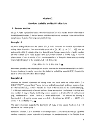
8. 8
= ෍ ܲ௑ሺሼ݅ሽሻ
௜ ∈ ሼ଴,ଵ,ଶ,ଷሽ∩஻
, ‫ܤ‬ ∈ ࣜଵ.
Clearly, for ‫ݔ‬ ∈ Թ,
‫ܨ‬௑ሺ‫ݔ‬ሻ ൌ ܲሺሼܺ ൑ ‫ݔ‬ሽ ሻ
ൌ ܲ௑ሺሺെ∞, ‫ݔ‬ሿ ሻ
ൌ ෍ ܲܺሺሼ݅ሽሻ
݅ ∈ ሼ0,1,2,3ሽ∩ሺିஶ,௫ሿ
ൌ
‫ە‬
ۖ
ۖ
‫۔‬
ۖ
ۖ
‫ۓ‬
0, if ‫ݔ‬ ൏ 0
1
8
, if 0 ൑ ‫ݔ‬ ൏ 1
1
2
, if 1 ൑ ‫ݔ‬ ൏ 2
7
8
, if 2 ൑ ‫ݔ‬ ൏ 3
1, if ‫ݔ‬ ൒ 3
Figure 3.1. Plot of distribution function ‫ܨ‬௑ሺ‫ݔ‬ሻ
Note that ‫ܨ‬௑ሺ‫ݔ‬ሻ is non-decreasing, right continuous, ‫ܨ‬௑ሺെ∞ሻ ≝ lim௫→ିஶ ‫ܨ‬௑ሺ‫ݔ‬ሻ ൌ 0
and ‫ܨ‬௑ሺ∞ሻ ≝ lim௫→ஶ ‫ܨ‬௑ሺ‫ݔ‬ሻ ൌ 1. Moreover ‫ܨ‬௑ሺ‫ݔ‬ሻ is a step function having
discontinuities at points 0, 1, 2 and 3.

9. 9
(ii) Consider Example 2.1 (ii). The probability space induced by r.v. ܺ is (Թ, ℬଵ, ܲ௑),
where, for ‫ܤ‬ ∈ ℬଵ,
ܲ௑ሺ‫ܤ‬ሻ = 2 න ‫ݖ‬
ஶ
଴
݁ି௭మ
‫ܫ‬஻ሺ‫ݖ‬ሻ݀‫.ݖ‬
Therefore,
‫ܨ‬௑ሺ‫ݔ‬ሻ = ܲሺሼܺ ≤ ‫ݔ‬ሽ ሻ
= ܲ௑ሺሺ−∞, ‫ ]ݔ‬ሻ
= 2 න ‫ݖ‬
∞
0
݁−‫ݖ‬2
‫ܫ‬ሺିஶ,௫]ሺ‫ݖ‬ሻ݀‫,ݖ‬ ‫ݔ‬ ∈ ℝ.
Clearly, for ‫ݔ‬ < 0, ‫ܨ‬௑ሺ‫ݔ‬ሻ = 0. For ‫ݔ‬ ≥ 0
‫ܨ‬௑ሺ‫ݔ‬ሻ = 2 න ‫ݖ‬
௫
଴
݁ି௭మ
݀‫ݖ‬ = 1 − ݁ି௫మ
.
Thus,
‫ܨ‬௑ሺ‫ݔ‬ሻ = ൜
0, if ‫ݔ‬ < 0
1 − ݁ି௫మ
, if ‫ݔ‬ ≥ 0
.
Note that ‫ܨ‬௑ሺ‫ݔ‬ሻ is non-decreasing, continuous, ‫ܨ‬௑ሺ−∞ሻ = lim௫→ିஶ ‫ܨ‬௑ሺ‫ݔ‬ሻ = 0 and
‫ܨ‬௑ሺ∞ሻ = lim௫→ ஶ ‫ܨ‬௑ሺ‫ݔ‬ሻ = 1. ▄
Now we will derive various properties of a distribution function. The following lemma, whose
proof is immediate and can be found in any standard text book on calculus, will be useful in
studying the properties of a distribution function.
Lemma 3.1
Let −∞ ≤ ܽ < ܾ ≤ ∞ and let ݂: ሺܽ, ܾሻ → ℝ be a non-decreasing functionሺi. e. , ݂ሺ‫ݏ‬ሻ ≤ ݂ሺ‫ݐ‬ሻ,
∀ ܽ < ‫ݏ‬ < ‫ݐ‬ < ܾሻ.
Then
(i) for all ‫ݔ‬ ∈ ሺܽ, ܾ] and ‫ݕ‬ ∈ [ܽ, ܾሻ, ݂ሺ‫ݔ‬ −ሻ and ݂ሺ‫ݕ‬ +ሻ exist;
(ii) for all ‫ݔ‬ ∈ ሺܽ, ܾሻ, ݂ሺ‫ݔ‬ −ሻ ≤ ݂ሺ‫ݔ‬ሻ ≤ ݂ሺ‫ݔ‬ +ሻ;
(iii) for ܽ < ‫ݔ‬ < ‫ݕ‬ < ܾ, ݂ሺ‫+ݔ‬ሻ ≤ ݂ሺ‫−ݕ‬ሻ;
(iv) ݂ has at most countable number of discontinuities;

10. 10
where ݂ሺܿ െሻ and ݂ሺܿ +ሻ denote, respectively, the left hand and right hand limits of the
function ݂ at point ܿ ∈ ሺܽ, ܾሻ. ▄
Theorem 3.1
Let ‫ܨ‬௑be the distribution function of a random variable ܺ. Then
(i) ‫ܨ‬௑ is non-decreasing;
(ii) ‫ܨ‬௑ is right continuous;
(iii) ‫ܨ‬௑ሺ−∞ሻ ≝ lim୶→ିஶ ‫ܨ‬௑ ሺ‫ݔ‬ሻ = 0 and ‫ܨ‬௑ሺ∞ሻ ≝ lim௫→ ஶ ‫ܨ‬௑ ሺ‫ݔ‬ሻ = 1.
Proof.
(i) Let −∞ < ‫ݔ‬ < ‫ݕ‬ < ∞ . Then ሺ−∞, ‫ݔ‬] ⊆ ሺ−∞, ‫]ݕ‬ and therefore, on using
monotonicity of probability measures, we get
‫ܨ‬௑ሺ‫ݔ‬ሻ = ܲ௑൫ሺ−∞, ‫ݔ‬]൯ ≤ ܲ௑ሺሺ−∞, ‫]ݕ‬ሻ = ‫ܨ‬௑ሺ‫ݕ‬ሻ.
(ii) Fix ‫ݔ‬ ∈ ℝ. Since ‫ܨ‬௑ is non-decreasing, it follows from Lemma 3.1 that ‫ܨ‬௑ሺ‫ݔ‬ +ሻ
exists. Therefore
‫ܨ‬௑ሺ‫ݔ‬ +ሻ = lim
௡→ ஶ
‫ܨ‬௑ ൬‫ݔ‬ +
1
݊
൰ = lim
௡→ ஶ
ܲ௑ ൬ሺ−∞, ‫ݔ‬ +
1
݊
]൰.
Note that ቀ−∞, ‫ݔ‬ +
ଵ
௡
ቃ ↓ and Lim௡→ ஶ ቀ−∞, ‫ݔ‬ +
ଵ
௡
ቃ = ⋂ ቀ−∞, ‫ݔ‬ +
ଵ
௡
ቃஶ
௡ୀଵ = ሺ−∞, ‫.]ݔ‬
Now using continuity of probability measures (Theorem 4.1, Module 1) we have
‫ܨ‬௑ሺ‫ݔ‬ +ሻ = lim
௡→ ஶ
ܲ௑ ൬ሺ−∞, ‫ݔ‬ +
1
݊
]൰
= ܲ௑ ቀLim
௡→ ஶ
ሺ−∞, ‫ݔ‬ +
ଵ
௡
]ቁ
= ܲ௑ሺሺ−∞, ‫]ݔ‬ሻ
= ‫ܨ‬௑ሺ‫ݔ‬ሻ.
(iii) Using standard arguments of calculus it follows that ‫ܨ‬௑ሺ−∞ሻ = lim
௡→ ஶ
‫ܨ‬௑ሺ−݊ሻ
and ‫ܨ‬௑ሺ∞ሻ = lim
௡→ ஶ
‫ܨ‬௑ሺ݊ሻ , where limits are taken along the sequence ሼ݊: ݊ =
1, 2, ⋯ ሽ. Note that ሺ−∞, −݊] ↓, ሺ−∞, ݊] ↑, Lim
௡→ ஶ
ሺ−∞, −݊] = ⋂ ሺ−∞, −݊]ஶ
௡ୀଵ = ߶
and Lim
௡→ ஶ
ሺ−∞, ݊] = ⋃ ሺ−∞, ݊]ஶ
୬ୀଵ = ℝ. Again using the continuity of probability
measures, we get
‫ܨ‬௑ሺ−∞ሻ = lim
௡→ ஶ
‫ܨ‬௑ሺ−݊ሻ = lim
௡→ ஶ
ܲ௑൫ሺ−∞, −݊]൯ = ܲ௑ ቀLim
௡→ ஶ
ሺ−∞, −݊]ቁ = ܲ௑ሺ߶ሻ = 0,
and

11. 11
‫ܨ‬௑ሺ∞ሻ = lim
௡→ ஶ
‫ܨ‬௑ሺ݊ሻ = lim
௡→ ஶ
ܲ௑൫ሺ−∞, ݊]൯ = ܲ௑ ቀLim
௡→ ஶ
ሺ−∞, ݊]ቁ = ܲ௑ሺℝሻ = 1. ▄
Remark 3.1
(i) Using Lemma-3.1 (i)-(ii) and Theorem 3.1 (i) it follows that for a d.f. ‫ܨ‬௑, ‫ܨ‬௑ሺ‫ݔ‬ +ሻ and
‫ܨ‬௑ሺ‫ݔ‬ −ሻexist for every ‫ ݔ‬ ∈ ℝ and ‫ܨ‬௑ is discontinuous at ‫ݔ‬ ∈ ℝ if and only if
‫ܨ‬௑ሺ‫ݔ‬ −ሻ < ‫ܨ‬௑ሺ‫ݔ‬ +ሻ = ‫ܨ‬௑ሺ‫ݔ‬ሻ. Consequently a d.f. has only jump discontinuities (a
discontinuity point ‫ݔ‬ ∈ ℝ of ‫ܨ‬௑is called a jump discontinuity if ‫ܨ‬௑ሺ‫ݔ‬ +ሻ and ‫ܨ‬௑ሺ‫ݔ‬ −ሻ
exist but ‫ܨ‬௑ሺ‫ݔ‬ −ሻ = ‫ܨ‬௑ሺ‫ݔ‬ +ሻ = ‫ܨ‬௑ሺ‫ݔ‬ሻ does not hold). Moreover the size of the jump
at a point ‫ݔ‬ ∈ ℝ of discontinuity is ‫݌‬௫ = ‫ܨ‬௑ሺ‫ݔ‬ሻ − ‫ܨ‬௑ሺ‫ݔ‬ −ሻ.
(ii) Using Lemma 3.1 (iv) and Theorem 3.1 (i) it follows that any d.f. ‫ܨ‬௑ has atmost
countable number of discontinuities.
(iii) Let ܽ ∈ ℝ . Since ሺ−∞, a −
ଵ
୬
] ↑ and Lim௡→ஶ ሺ−∞, a −
ଵ
୬
] = ⋃ ሺ−∞, a −
ଵ
୬
] ஶ
௡ୀଵ =
ሺ−∞, ܽሻ, the continuity of probability measures implies
ܲሺሼܺ < ܽሽሻ = ܲ௑൫ሺ−∞, ܽሻ൯
= ܲ௑ ቆLim
௡→ஶ
ሺ−∞, a −
1
n
] ቇ
= lim
௡→ஶ
ܲ௑ ቆሺ−∞, a −
1
n
] ቇ
= lim
௡→ஶ
‫ܨ‬௑ ൬ܽ −
1
݊
൰
= ‫ܨ‬௑ሺܽ −ሻ.
Therefore,
Pሺሼܺ < ‫ݔ‬ሽሻ = ‫ܨ‬௑ሺ‫ݔ‬ −ሻ, ∀ ‫ݔ‬ ∈ ℝ.
Also,
‫ܨ‬௑ሺ‫ݔ‬ሻ = ‫ܨ‬௑ሺ‫ݔ‬ +ሻ ≤ ‫ܨ‬௑ሺ‫ݕ‬ −ሻ, ∀ − ∞ < ‫ݔ‬ < ‫ݕ‬ < ∞ ሺusing Lemma 3.1 ሺiiiሻሻ
and
ܲሺሼܺ = ‫ݔ‬ሽሻ = ܲሺሼܺ ≤ ‫ݔ‬ሽሻ − ܲሺሼܺ < ‫ݔ‬ሽሻ = ‫ܨ‬௑ሺ‫ݔ‬ሻ − ‫ܨ‬௑ሺ‫ݔ‬ −ሻ, ∀ ‫ ݔ‬ ∈ ℝ.
Thus ‫ܨ‬௑ is continuous (discontinuous) at a point ‫ ݔ‬ ∈ ℝ if, and only if, ܲሺሼܺ = ‫ݔ‬ሽሻ =
0 ሺܲሺሼܺ = ‫ݔ‬ሽሻ > 0ሻ.
(iv) Let ‫ܦ‬௑ denote the set of discontinuity points (jump points) of d.f. ‫ܨ‬௑. Then ‫ܦ‬௑ is a
countable set and
෍ [‫ܨ‬௑ሺ‫ݔ‬ሻ − ‫ܨ‬௑ሺ‫ݔ‬ −ሻ]
௫ ∈ ஽೉
= ෍ ܲሺሼܺ = ‫ݔ‬ሽሻ
௫ ∈ ஽೉
= ܲ௑ሺ‫ܦ‬௑ሻ ≤ 1,

12. 12
i.e., the sum of sizes of jumps of a d.f. does not exceed 1.
(v) Let െ∞ < ܽ < ܾ < ∞. Then
ܲሺሼܽ < ܺ ≤ ܾሽሻ = ܲሺሼܺ ≤ ܾሽሻ − ܲሺሼܺ ≤ ܽሽሻ = ‫ܨ‬௑ሺܾሻ − ‫ܨ‬௑ሺܽሻ
ܲሺሼܽ < ܺ < ܾሽሻ = ܲሺሼܺ < ܾሽሻ − ܲሺሼܺ ≤ ܽሽሻ = ‫ܨ‬௑ሺܾ −ሻ − ‫ܨ‬௑ሺܽሻ
ܲሺሼܽ ≤ ܺ < ܾሽሻ = ܲሺሼܺ < ܾሽሻ − ܲሺሼܺ < ܽሽሻ = ‫ܨ‬௑ሺܾ −ሻ − ‫ܨ‬௑ሺܽ−ሻ
ܲሺሼܽ ≤ ܺ ≤ ܾሽሻ = ܲሺሼܺ ≤ ܾሽሻ − ܲሺሼܺ < ܽሽሻ = ‫ܨ‬௑ሺܾሻ − ‫ܨ‬௑ሺܽ −ሻ,
and, for −∞ < ܽ < ∞,
ܲሺሼܺ ≥ ܽሽሻ = 1 − ܲሺሼܺ < ܽሽሻ = 1 − ‫ܨ‬௑ሺܽ −ሻ,
and ܲሺሼܺ > ܽሽሻ = 1 − ܲሺሼܺ ≤ ܽሽሻ = 1 − ‫ܨ‬௑ሺܽሻ. ▄
We state the following theorem without providing the proof. The theorem essentially states
that any function ‫:ܩ‬ ℝ → ℝ that is non-decreasing and right continuous with ‫ܩ‬ሺ−∞ሻ =
lim௫→ିஶ ‫ܩ‬ሺ‫ݔ‬ሻ = 0 and ‫ܩ‬ሺ∞ሻ = lim௫→ஶ ‫ܩ‬ሺ‫ݔ‬ሻ = 1 can be regarded as d.f. of a random variable.
Theorem 3.2
Let ‫:ܩ‬ ℝ → ℝ be a non-decreasing and right continuous function for which ‫ܩ‬ሺ−∞ሻ = 0 and
‫ܩ‬ሺ∞ሻ = 1. Then there exists a random variable ܺ defined on a probability space ሺߗ, ℱ, ܲሻ such
that the distribution function of ܺ is ‫.ܩ‬ ▄
Example 3.2
(i) Consider a function‫:ܩ‬ ℝ → ℝ, defined by,
‫ܩ‬ሺ‫ݔ‬ሻ = ൜
0, if ‫ݔ‬ < 0
1 − ݁ି௫
, if ‫ݔ‬ ≥ 0
.

13. 13
Figure 3.2. Plot of distribution function ‫ܩ‬ሺ‫ݔ‬ሻ
Clearly ‫ܩ‬is non-decreasing, continuous and satisfies ‫ܩ‬ሺെ∞ሻ ൌ 0 and ‫ܩ‬ሺ∞ሻ ൌ 1.
Therefore G can be treated as d.f. of some r.v., say ܺ. Since ‫ܩ‬ is continuous we have
ܲሺሼܺ ൌ ‫ݔ‬ሽሻ ൌ ‫ܩ‬ሺ‫ݔ‬ሻ െ ‫ܩ‬ሺ‫ݔ‬ െሻ ൌ 0, ∀ ‫ݔ‬ ∈ Թ,
and, for െ∞ ൏ ܽ ൏ ܾ ൏ ∞,
ܲሺሼܽ ൏ ܺ ൏ ܾሽሻ ൌ ܲሺሼܽ ൑ ܺ ൏ ܾሽሻ ൌ Pሺܽ ൑ ܺ ൑ ܾሻ ൌ ܲሺሼܽ ൏ ܺ ൑ ܾሽሻ
ൌ ‫ܩ‬ሺܾሻ െ Gሺaሻ.
Moreover, for െ∞ ൏ ܽ ൏ ∞,
ܲሺሼܺ ൒ ܽሽሻ ൌ ܲሺሼܺ ൐ ܽሽሻ ൌ 1 െ ‫ܩ‬ሺܽሻ
and
ܲሺሼܺ ൏ ܽሽሻ ൌ ܲሺሼܺ ൑ ܽሽሻ ൌ ‫ܩ‬ሺܽሻ.
In particular
ܲሺሼ2 ൏ ܺ ൑ 3ሽሻ ൌ ‫ܩ‬ሺ3ሻ െ ‫ܩ‬ሺ2ሻ ൌ ݁ିଶ
െ ݁ିଷ
;
ܲሺሼെ2 ൏ ܺ ൑ 3ሽሻ ൌ ‫ܩ‬ሺ3ሻ െ ‫ܩ‬ሺെ2ሻ ൌ 1 െ ݁ିଷ
;
ܲሺሼ1 ൑ ܺ ൏ 4ሽሻ ൌ ‫ܩ‬ሺ4ሻ െ ‫ܩ‬ሺ1ሻ ൌ ݁ିଵ
െ ݁ିସ
;
ܲሺሼ5 ൑ ܺ ൏ 8ሽሻ ൌ ‫ܩ‬ሺ8ሻ െ ‫ܩ‬ሺ5ሻ ൌ ݁ିହ
െ ݁ି଼
;
ܲሺሼܺ ൒ 2ሽሻ ൌ 1 െ ‫ܩ‬ሺ2ሻ െ ݁ିଶ
;

14. 14
and
ܲሺሼܺ ൐ 5ሽሻ ൌ 1 െ ‫ܩ‬ሺ5ሻ ൌ ݁ିହ
.
Note that the sum of sizes of jumps of ‫ܩ‬ is 0.
(ii) Let ‫:ܪ‬ Թ → Թ be given by
‫ܪ‬ሺ‫ݔ‬ሻ ൌ
‫ە‬
ۖۖ
‫۔‬
ۖۖ
‫ۓ‬
0, if ‫ݔ‬ ൏ 0
௫
ସ
, if 0 ൑ ‫ݔ‬ ൏ 1
௫
ଷ
if 1 ൑ ‫ݔ‬ ൏ 2
ଷ௫
଼
if 2 ൑ ‫ݔ‬ ൏
ହ
ଶ
1, if ‫ݔ‬ ൒
ହ
ଶ
.
Figure 3.3. Plot of distribution function ‫ܪ‬ሺ‫ݔ‬ሻ
Clearly ‫ܪ‬ is non-decreasing, right continuous and satisfies ‫ܪ‬ሺെ∞ሻ ൌ 0 and
‫ܪ‬ሺ∞ሻ ൌ 1 . Therefore ‫ܪ‬ can be treated as d.f. of some r.v., say ܻ .
‫ܪ‬is continuous everywhere except at points 1, 2, and 5/2 where it has jump
discontinuities with jumps of sizes ܲሺሼܻ ൌ 1ሽሻ ൌ ‫ܪ‬ሺ1ሻ െ ‫ܪ‬ሺ1 െሻ ൌ 1/
12, ܲሺሼܻ ൌ 2ሽሻ ൌ ‫ܪ‬ሺ2ሻ െ ‫ܪ‬ሺ2 െሻ ൌ 1/12 and ܲሺሼܻ ൌ 5/2ሽሻ ൌ ‫ܪ‬ሺ5/2ሻ െ
‫ܪ‬ሺ5/2െሻ ൌ 1/16. Moreover for ‫ݔ‬ ∈ Թ െ ሼ1, 2, 5/2ሽ, ܲሺሼܻ ൌ ‫ݔ‬ሽሻ ൌ 0. We also
have
ܲ ൬൜1 ൏ ܻ ൑
5
2
ൠ൰ ൌ ‫ܪ‬ ൬
5
2
൰ െ ‫ܪ‬ሺ1ሻ ൌ 1 െ
1
3
ൌ
2
3
;

15. 15
ܲ ൬൜1 ൏ ܻ ൏
5
2
ൠ൰ ൌ ‫ܪ‬ ൬
5
2
െ൰ െ ‫ܪ‬ሺ1ሻ ൌ
15
16
െ
1
3
ൌ
29
48
;
ܲ ቀቄ1 ൑ ܻ ൏
ହ
ଶ
ቅቁ ൌ ‫ܪ‬ ቀ
ହ
ଶ
െቁ െ ‫ܪ‬ሺ1 െሻ ൌ
ଵହ
ଵ଺
െ
ଵ
ସ
ൌ
ଵଵ
ଵ଺
;
ܲሺሼെ2 ൑ ܻ ൏ 1ሽሻ ൌ ‫ܪ‬ሺ1 െሻ െ ‫ܪ‬ሺെ2 െሻ ൌ
ଵ
ସ
െ 0 ൌ
ଵ
ସ
;
ܲሺሼܻ ൒ 2ሽሻ ൌ 1 െ ‫ܪ‬ሺ2 െሻ ൌ 1 െ
2
3
ൌ
1
3
;
and ܲሺሼܻ ൐ 2ሽሻ ൌ 1 െ ‫ܪ‬ሺ2ሻ ൌ 1 െ
ଷ
ସ
ൌ
ଵ
ସ
∙
Note that sum of sizes of jumps of ‫ܪ‬ is 11/48 ∈ ሺ0, 1ሻ.
(iii) Let ‫:ܨ‬ Թ → Թ be given by
‫ܨ‬ሺ‫ݔ‬ሻ ൌ
‫ە‬
ۖ
ۖ
ۖ
‫۔‬
ۖ
ۖ
ۖ
‫ۓ‬
0, if ‫ݔ‬ ൏ 0
ଵ
଼
, if 0 ൑ ‫ݔ‬ ൏ 2
ଵ
ସ
if 2 ൑ ‫ݔ‬ ൏ 3
ଵ
ଶ
if 3 ൑ ‫ݔ‬ ൏ 6
ସ
ହ
, if 6 ൑ ‫ݔ‬ ൏ 12
଻
଼
, if 12 ൑ ‫ݔ‬ ൏ 15
1, if ‫ݔ‬ ൒ 15
.
Figure 3.4. Plot of distribution function ‫ܨ‬ሺ‫ݔ‬ሻ

16. 16
As ‫ܨ‬ is non-decreasing and right continuous with ‫ܨ‬ሺെ∞ሻ = 0 and ‫ܨ‬ሺ∞ሻ = 1, it can
be regarded as d.f. of some r.v., say ܼ. Clearly, except at points 0, 2, 3, 6, 12 and 15,
‫ܨ‬ is continuous at all other points and at discontinuity points 0, 2, 3, 6 ,12 and15 it
has jump discontinuities with jumps of sizes
ܲሺሼܼ = 0ሽሻ = ‫ܨ‬ሺ0ሻ − ‫ܨ‬ሺ0 −ሻ =
1
8
,
ܲሺሼܼ = 2ሽሻ = ‫ܨ‬ሺ2ሻ − ‫ܨ‬ሺ2 −ሻ =
1
8
,
ܲሺሼܼ = 3ሽሻ = ‫ܨ‬ሺ3ሻ − ‫ܨ‬ሺ3 −ሻ =
1
4
,
ܲሺሼܼ = 6ሽሻ = ‫ܨ‬ሺ6ሻ − ‫ܨ‬ሺ6 −ሻ =
3
10
,
ܲሺሼܼ = 12ሽሻ = ‫ܨ‬ሺ12ሻ − ‫ܨ‬ሺ12 −ሻ =
3
40
,
and
ܲሺሼܼ = 15ሽሻ = ‫ܨ‬ሺ15ሻ − ‫ܨ‬ሺ15 −ሻ =
1
8
.
Moreover ܲሺሼܼ = ‫ݔ‬ሽሻ = ‫ܨ‬ሺ‫ݔ‬ሻ = ‫ܨ‬ሺ‫ݔ‬ −ሻ = 0, ∀ ‫ ݔ‬ ∈ ℝ − ሼ0, 2, 3, 6, 12, 15ሽ. Note
that in this case sum of sizes of jumps of ‫ܨ‬ is 1. ▄
Remark 3.2
Let ܺ be a r.v. defined on a probability space ሺߗ, ℱ, ܲሻ and let ሺℝ, ‫ܤ‬ଵ, ܲ௑ሻ be the probability
space induced by ܺ. In advanced courses on probability theory it is shown that the d.f. ‫ܨ‬௑
uniquely determines the induced probability measure ܲ௑ and vice-versa. Thus to study the
induced probability space ሺℝ, ‫ܤ‬ଵ, ܲ௑ሻ it suffices to study the d.f. ‫ܨ‬௑. ▄
4. Types of Random Variables: Discrete, Continuous and Absolutely Continuous
Let ܺ be a r.v. defined on a probability space ሺߗ, ℱ, ܲሻ and let ሺℝ, ‫ܤ‬ଵ, ܲ௑ሻbe the probability
space induced by ܺ. Let ‫ܨ‬௑ be the d.f. of ܺ. Then ‫ܨ‬௑ will either be continuous everywhere or it
will have countable number of discontinuities. Moreover the sum of sizes of jumps at the point
of discontinuities of ‫ܨ‬௑ will be either 1 or less than 1. These properties can be used to classify a
r.v. into three broad categories.
Definition 4.1

17. 17
A random variable ܺ is said to be of discrete type if there exists a non-empty and countable set
ܵ௑ such that ܲሺሼܺ ൌ ‫ݔ‬ሽሻ ൌ ‫ܨ‬௑ሺ‫ݔ‬ሻ െ ‫ܨ‬௑ሺ‫ݔ‬ െሻ ൐ 0, ∀ ‫ ݔ‬ ∈ ܵ௑ and ܲ௑ሺܵ௑ሻ = ∑ ܲ௫∈ௌ೉
ሺሼܺ =
‫ݔ‬ሽሻ = ∑ [‫ܨ‬௑ሺ‫ݔ‬ሻ − ‫ܨ‬௑ሺ‫ݔ‬ −ሻ]௫∈ௌ೉
= 1. The set ܵ௑ is called the support of the discrete random
variable ܺ. ▄
Remark 4.1
If a r.v. ܺ is of discrete type then ܲ௑ሺܵ௑
஼ሻ = 1 − ܲ௑ሺܵ௑ሻ = 0 and, consequently ܲሺሼܺ = ‫ݔ‬ሽሻ =
0, ∀ ‫ ݔ‬ ∈ ܵ௑
஼
, i. e. , ‫ܨ‬௑ሺ‫ݔ‬ሻ − ‫ܨ‬௑ሺ‫ݔ‬ −ሻ = 0, ∀ ‫ ݔ‬ ∈ ܵ௑
஼
and ‫ܨ‬௑ is continuous at every point of
ܵ௑
஼
.Moreover, ‫ܨ‬௑ሺ‫ݔ‬ሻ − ‫ܨ‬௑ሺ‫ݔ‬ −ሻ = ܲሺሼܺ = ‫ݔ‬ሽሻ > 0, ∀ ‫ ݔ‬ ∈ Sଡ଼. It follows that the support ܵ௑
of a discrete type r.v. ܺ is nothing but the set of discontinuity points of the d.f. ‫ܨ‬௑. Moreover
the sum of sizes of jumps at the point of discontinuities is
∑ [‫ܨ‬௑ሺ‫ݔ‬ሻ − ‫ܨ‬௑ሺ‫ݔ‬ −ሻ]௫∈ௌೣ
= ∑ ܲሺሼܺ = ‫ݔ‬ሽሻ௫∈ௌೣ
= ܲ௑ሺܵ௑ሻ = 1. ▄
Thus we have the following theorem.
Theorem 4.1
Let ܺ be a random variable with distribution function ‫ܨ‬௑ and let ‫ܦ‬௑ be the set of discontinuity
points of ‫ܨ‬௑. Then ܺ is of discrete type if, and only if, ܲሺሼܺ ∈ ‫ܦ‬௑ሽሻ = 1. ▄
Definition 4.2
Let ܺ be a discrete type random variable with support ܵ௑. The function ݂௑: ℝ → ℝ, defined by,
݂௑ሺ‫ݔ‬ሻ = ൜
ܲሺሼܺ = ‫ݔ‬ሽሻ, if ‫ݔ‬ ∈ ܵ௑
0, otherwise
is called the probability mass function (p.m.f.) of ܺ.
Example 4.1
Let us consider a r.v. ܼ having the d.f. ‫ܨ‬ considered in Example 3.2 (iii). The set of discontinuity
points of ‫ܨ‬ is ‫ܦ‬௓ = ሼ0, 2, 3, 6, 12, 15ሽ and ܲሺሼܼ ∈ ‫ܦ‬௓ሽሻ = ∑ [‫ܨ‬ሺ‫ݖ‬ሻ − ‫ܨ‬ሺ‫ݖ‬ −ሻ]௭∈ ஽ೋ
= 1.
Therefore the r.v. ܼ is of discrete type with support ܵ௓ = ‫ܦ‬௓ = ሼ0, 2, 3, 6, 12, 15ሽ and p.m.f.
݂௓ሺ‫ݖ‬ሻ = ൜
[‫ܨ‬ሺ‫ݖ‬ሻ − ‫ܨ‬ሺ‫ݖ‬ −ሻ], if ‫ ݖ‬ ∈ ܵ௓
0, otherwise

18. 18
ൌ
‫ە‬
ۖ
ۖ
ۖ
‫۔‬
ۖ
ۖ
ۖ
‫ۓ‬
1
8
, if ‫ ݖ‬ ∈ ሼ0, 2, 15ሽ
1
4
, if ‫ݖ‬ ൌ 3
3
10
, if ‫ݖ‬ ൌ 6
3
40
, if ‫ݖ‬ ൌ 12
0, otherwise
.
Figure 4.1. Plot of p.m.f. ݂௓ሺ‫ݖ‬ሻ
Note that the p.m.f. ݂௑ of a discrete type r.v. ܺ, having support ܵ௑, satisfies the following
properties:
(i) ݂௑ሺ‫ݔ‬ሻ ൐ 0, ∀ ‫ ݔ‬ ∈ ܵ௑ and ݂௑ሺ‫ݔ‬ሻ ൌ 0, ∀ ‫ ݔ‬ ∉ ܵ௑, (4.1)
(ii) ∑ ݂௑ሺ‫ݔ‬ሻ ൌ௫ ∈ ௌ೉
∑ ܲሺሼܺ ൌ ‫ݔ‬ሽሻ௫ ∈ ௌ೉
ൌ 1. (4.2)
Moreover, for ‫ܤ‬ ∈ ࣜଵ,
ܲ௑ሺ‫ܤ‬ሻ ൌ ܲ௑ሺ‫ܤ‬ ∩ ܵ௑ሻ + ܲ௑ሺ‫ܤ‬ ∩ ܵ௑
஼ሻ
ൌ ܲ௑ሺ‫ܤ‬ ∩ ܵ௑ሻ (since ‫ܤ‬ ∩ ܵ௑
஼
⊆ ܵ௑
஼
and ܲ௑ሺܵ௑
஼ሻ ൌ 0)
ൌ ෍ ݂௑ሺ‫ݔ‬ሻ
௫ ∈஻∩ௌ೉
.
This suggest that we can study probability space ሺԹ, ࣜଵ, ܲ௑ሻ, induced by a discrete type r.v. ܺ,
through the study of its p.m.f. ݂௑. Also
‫ܨ‬௑ሺ‫ݔ‬ሻ ൌ ෍ ݂௑
௬ ∈ሺିஶ,௫ሿ∩ௌ೉
ሺ‫ݕ‬ሻ, ‫ݔ‬ ∈ Թ
and

19. 19
݂௑ሺ‫ݔ‬ሻ ൌ ܲሺሼܺ ൌ ‫ݔ‬ሽሻ ൌ ‫ܨ‬௑ሺ‫ݔ‬ሻ െ ‫ܨ‬௑ሺ‫ݔ‬ െሻ, ‫ݔ‬ ∈ ℝ.
Thus, given a p.m.f. of a discrete type of r.v., we can get its d.f. and vice-versa. In other words,
there is one-one correspondence between p.m.f.s and distribution functions of discrete type
random variables.
The following theorem establishes that any function ݃: ℝ → ℝ satisfying (4.1) and (4.2) is p.m.f.
of some discrete type random variable.
Theorem 4.2
Suppose that there exists a non-empty and countable set ܵ ⊆ ℝ and a function ݃: ℝ → ℝ
satisfying: (i) ݃ሺ‫ݔ‬ሻ > 0, ∀‫ ݔ‬ ∈ ܵ; (ii)݃ሺ‫ݔ‬ሻ = 0, ∀‫ݔ‬ ∉ ܵ, and (iii) ∑ ݃ሺ‫ݔ‬ሻ௫ ∈ௌ = 1. Then there
exists a discrete type random variable on some probability space ሺℝ, ℬଵ, ܲሻ such that the p.m.f.
of ܺ is ݃.
Proof. Define the set function ܲ: ℬଵ → ℝ by
ܲሺ‫ܤ‬ሻ = ෍ ݃ሺ‫ݔ‬ሻ
௫ ∈஻∩ௌ
, ‫ܤ‬ ∈ ℬଵ.
It is easy to verify that ܲ is a probability measure on ℬଵ, i.e., ሺℝ, ℬଵ, ܲሻis a probability space.
Define ܺ: ℝ → ℝ by ܺሺ߱ሻ = ߱, ߱ ∈ ℝ. Clearly ܺ is a r.v. on the probability space ሺℝ, ℬଵ, ܲሻ and
it induces the same probability space ሺℝ, ℬଵ, ܲሻ. Clearly ܲሺሼܺ = ‫ݔ‬ሽሻ = ݃ሺ‫ݔ‬ሻ, ‫ ݔ‬ ∈ ℝ, and
∑ ݃ሺ‫ݔ‬ሻ௫ ∈ௌ = 1. Therefore the r.v. ܺ is of discrete type with support ܵ and p.m.f. ݃. ▄
Example 4.2
Consider a coin that, in any flip, ends up in head with probability
ଵ
ସ
and in tail with probability
ଷ
ସ
.
The coin is tossed repeatedly and independently until a total of two heads have been observed.
Let ܺ denote the number of flips required to achieve this. Then ܲሺሼܺ = ‫ݔ‬ሽሻ = 0, if ‫ݔ‬ ∉
ሼ2, 3, 4, ⋯ ሽ. For ݅ ∈ ሼ2, ,3 ,4 … ሽ
ܲሺሼܺ = ݅ሽሻ = ቌቀ
݅ − 1
1
ቁ
1
4
൬
3
4
൰
௜ିଶ
ቍ
1
4
=
݅ − 1
16
൬
3
4
൰
௜ିଶ
.
Moreover, ∑ ܲሺሼܺ = ݅ሽሻஶ
௜ୀଶ = 1. It follows that ܺ is a discrete type r.v. with support
ܵ௑ = ሼ2, 3, 4, … ሽ and p.m.f.

20. 20
݂௑ሺ‫ݔ‬ሻ ൌ ൝
௫ିଵ
ଵ଺
ቀ
ଷ
ସ
ቁ
௫ିଶ
, if ‫ ݔ‬ ∈ ሼ2, 3, 4, ⋯ ሽ
0, otherwise
.
Figure 4.2. Plot of p.m.f. ݂௑ሺ‫ݔ‬ሻ
The d.f. of ܺ is
‫ܨ‬௑ሺ‫ݔ‬ሻ ൌ ܲሺሼܺ ൑ ‫ݔ‬ሽሻ
ൌ ൞
0, if ‫ݔ‬ ൏ 2
1
16
෍ሺ݆ െ 1ሻ ൬
3
4
൰
௝ିଶ௜
௝ୀଶ
, if ݅ ൑ ‫ݔ‬ ൏ ݅ + 1, ݅ ൌ 2, 3, 4, ⋯
ൌ ቐ
0, if ‫ݔ‬ ൏ 2
1 െ
݅ + 3
4
൬
3
4
൰
௜ିଵ
, if ݅ ൑ ‫ݔ‬ ൏ ݅ + 1, ݅ ൌ 2, 3, 4, ⋯
▄
Example 4.3
A r.v. ܺ has the d.f.

21. 21
‫ܨ‬௑ሺ‫ݔ‬ሻ ൌ
‫ە‬
ۖ
ۖ
ۖ
‫۔‬
ۖ
ۖ
ۖ
‫ۓ‬
0, if ‫ݔ‬ < 2
ଶ
ଷ
, if 2 ≤ ‫ݔ‬ < 5
଻ି଺௞
଺
, if 5 ≤ ‫ݔ‬ < 9
ଷ௞మି଺௞ା଻
଺
, if 9 ≤ ‫ݔ‬ < 14
ଵ଺௞మିଵ଺௞ାଵଽ
ଵ଺
, if 14 ≤ ‫ݔ‬ ≤ 20
1, if ‫ݔ‬ > 20
,
where ݇ ∈ ℝ.
(i) Find the value of constant ݇;
(ii) Show that the r.v. ܺ is of discrete type and find its support;
(iii) Find the p.m.f. of ܺ.
Solution. (i) Since ‫ܨ‬௑ is right continuous, we have
‫ܨ‬௑ሺ20ሻ = ‫ܨ‬௑ሺ20+ሻ
⇒ 16݇ଶ
− 16݇ + 3 = 0
⇒ ݇ =
1
4
or ݇ =
3
4
. ሺ4.3ሻ
Also ‫ܨ‬௑ is non-decreasing. Therefore
‫ܨ‬௑ሺ5 −ሻ ≤ ‫ܨ‬௑ሺ5ሻ
⇒ ݇ ≤
1
2
. ሺ4.4ሻ
On combining (4.3) and (4.4) we get ݇ = 1/4. Therefore
‫ܨ‬௑ሺ‫ݔ‬ሻ =
‫ە‬
ۖۖ
‫۔‬
ۖۖ
‫ۓ‬
0, if ‫ݔ‬ < 2
ଶ
ଷ
, if 2 ≤ ‫ݔ‬ < 5
ଵଵ
ଵଶ
, if 5 ≤ ‫ݔ‬ < 9
ଽଵ
ଽ଺
, if 9 ≤ ‫ݔ‬ < 14
1, if ‫ݔ‬ ≥ 14
.
(ii) The set of discontinuity points of ‫ܨ‬௑ is ‫ܦ‬௑ = ሼ2, 5, 9, 14ሽ. Moreover
ܲሺሼܺ = 2ሽሻ = ‫ܨ‬௑ሺ2ሻ– ‫ܨ‬௑ሺ2 −ሻ =
ଶ
ଷ
,
ܲሺሼܺ = 5ሽሻ = ‫ܨ‬௑ሺ5ሻ– ‫ܨ‬௑ሺ5 −ሻ =
ଵ
ସ
,
ܲሺሼܺ = 9ሽሻ = ‫ܨ‬௑ሺ9ሻ– ‫ܨ‬௑ሺ9 −ሻ =
ଵ
ଷଶ
,

22. 22
ܲሺሼܺ ൌ 14ሽሻ = ‫ܨ‬௑ሺ14ሻ– ‫ܨ‬௑ሺ14 −ሻ =
ହ
ଽ଺
,
and ܲሺሼܺ ∈ ‫ܦ‬௑ሽሻ = ܲሺሼܺ = 2ሽሻ + ܲሺሼܺ = 5ሽሻ + ܲሺሼܺ = 9ሽሻ + ܲሺሼܺ = 14ሽሻ = 1.
Therefore the r.v. ܺ is of discrete type with support ܵ௑ = ሼ2, 5, 9, 14ሽ.
(iii) Clearly the p.m.f. of ܺ is given by
݂௑ሺ‫ݔ‬ሻ = ܲሺሼܺ = ‫ݔ‬ሽሻ =
‫ە‬
ۖ
ۖ
‫۔‬
ۖ
ۖ
‫ۓ‬
ଶ
ଷ
, if ‫ݔ‬ = 2
ଵ
ସ
, if ‫ݔ‬ = 5
ଵ
ଷଶ
, if ‫ݔ‬ = 9
ହ
ଽ଺
, if ‫ݔ‬ = 14
0, otherwise
.
▄
Example 4.4
A r.v. ܺ has the p.m.f.
݂௑ሺ‫ݔ‬ሻ = ൝
ܿ
ሺ2‫ݔ‬ − 1ሻሺ2‫ݔ‬ + 1ሻ
, if ‫ ݔ‬ ∈ ሼ1, 2, 3, ⋯ ሽ
0, otherwise
,
where ܿ ∈ ℝ.
(i) Find the value of constant ܿ;
(ii) For positive integers ݉ and ݊, such that ݉ < ݊, evaluate ܲሺሼܺ < ݉ + 1ሽሻ, ܲሺሼܺ ≥
݉ሽሻ, ܲሺሼ݉ ≤ ܺ < ݊ሽሻ and ܲሺሼ݉ < ܺ ≤ ݊ሽሻ;
(iii) Determine the d.f. of ܺ.
Solution.
(i) Let ܵ௑ be the support of ܺ so that ܵ௑ = ሼ‫ݔ‬ ∈ ℝ: ݂௑ሺ‫ݔ‬ሻ > 0ሽ and ∑ ݂௑ሺ‫ݔ‬ሻ = 1௫ ∈ௌ೉
.
Clearly, ܵ௑ = ሼ1, 2, 3, … ሽ and
෍
c
ሺ2݅ − 1ሻሺ2݅ + 1ሻ
= 1
ஶ
௜ୀଵ
⇒ lim
݊→∞
෍
ܿ
ሺ2݅ − 1ሻሺ2݅ + 1ሻ
= 1
௡
௜ୀଵ
⇒
ܿ
2
lim
݊→∞
෍ ൤
1
2݅ − 1
−
1
2݅ + 1
൨
௡
௜ୀଵ
= 1

23. 23
⇒
ܿ
2
lim
݊→∞
൥෍
1
2݅ − 1
− ෍
1
2݅ + 1
௡
௜ୀଵ
௡
௜ୀଵ
൩
௡
= 1
⇒
ܿ
2
lim
݊→∞
൤1 −
1
2݊ + 1
൨ = 1
⇒ c = 2.
(ii) We have
ܲሺሼܺ < ݉ + 1ሽሻ = ܲሺሼܺ ≤ ݉ሽሻ
= ෍
2
ሺ2݅ − 1ሻሺ2݅ + 1ሻ
௠
௜ୀଵ
= ෍ ൤
1
2݅ − 1
−
1
2݅ + 1
൨
௠
௜ୀଵ
= 1 −
1
2݉ + 1
=
2݉
2݉ + 1
,
ܲሺሼܺ ≥ ݉ሽሻ = 1 − ܲሺሼܺ < ݉ሽሻ
= 1 −
2ሺ݉ − 1ሻ
2ሺ݉ − 1ሻ + 1
=
1
2݉ − 1
,
ܲሺሼ݉ ≤ ܺ < ݊ሽሻ = ܲሺሼܺ < ݊ሽሻ − ܲሺሼܺ < ݉ሽሻ
=
2ሺ݊ − 1ሻ
2݊ − 1
−
2ሺ݉ − 1ሻ
2݉ − 1
=
2ሺ݊ − ݉ሻ
ሺ2݊ − 1ሻሺ2݉ − 1ሻ
,
and ܲሺሼ݉ < ܺ ≤ ݊ሽሻ = ܲሺሼ݉ + 1 ≤ ܺ < ݊ + 1ሽሻ
=
2ሺ݊ − ݉ሻ
ሺ2݊ + 1ሻሺ2݉ + 1ሻ
.
(iii) Clearly, for ‫ݔ‬ < 1, ‫ܨ‬௑ሺ‫ݔ‬ሻ = 0. For ݅ ≤ ‫ݔ‬ < ݅ + 1, ݅ = 1, 2, 3, ⋯

24. 24
‫ܨ‬௑ሺ‫ݔ‬ሻ ൌ ܲሺሼܺ ൏ ݅ + 1ሽሻ =
2݅
2݅ + 1
. ሺusingሺiiሻሻ
Therefore,
‫ܨ‬௑ሺ‫ݔ‬ሻ = ൝
0, if ‫ݔ‬ < 1
2݅
2݅ + 1
, if ݅ ≤ ‫ݔ‬ < ݅ + 1, ݅ = 1, 2, 3, ⋯
. ▄
Definition 4.3
(i) A random variable ܺ is said to be of continuous type if its distribution function ‫ܨ‬௑ is
continuous everywhere.
(ii) A random variable ܺ with distribution function ‫ܨ‬௑ is said to be of absolutely
continuous type if there exists an integrable function ݂௑: ℝ → ℝ such that
݂௑ሺ‫ݔ‬ሻ ≥ 0, ∀‫ݔ‬ ∈ ℝ, and
‫ܨ‬௑ሺ‫ݔ‬ሻ = න ݂௫ሺtሻ݀‫,ݐ‬
௫
ିஶ
‫ݔ‬ ∈ ℝ.
The function ݂௑ is called the probability density function (p.d.f.) of random variable ܺ
and the set ܵ௑ = ሼ‫ݔ‬ ∈ ℝ: ݂௑ሺ‫ݔ‬ሻ > 0ሽ is called the support of random variable ܺ (or
of p.d.f. ݂௑ ). ▄
Note that if ݂௑ is p.d.f. of an absolutely continuous type r.v. ܺ then ݂௑ሺ‫ݔ‬ሻ ≥ 0, ∀‫ݔ‬ ∈
ℝ and ‫׬‬ ݂௑ሺtሻ݀‫ݐ‬
ஶ
ିஶ
= ‫ܨ‬௑ሺ∞ሻ = 1, where ‫ܨ‬௑ሺ∞ሻ = lim
‫∞→ݔ‬
‫ܨ‬௑ሺ‫ݔ‬ሻ.
Example 4.5
Let ܺ be a r.v. having the d.f.
‫ܨ‬௑ሺ‫ݔ‬ሻ = ൜
0, if ‫ݔ‬ < 0
1 − ݁ି௫
, if ‫ݔ‬ ≥ 0
.
Clearly ‫ܨ‬௑ is continuous at every ‫ݔ‬ ∈ ℝ and therefore ܺ is of continuous type. Also
‫ܨ‬௑ሺ‫ݔ‬ሻ = ‫׬‬ ݂௑
௫
ିஶ
ሺtሻ ݀‫ݔ ,ݐ‬ ∈ ℝ,
where ݂௑: ℝ → [0, ∞ሻ is given by
݂௑ሺ‫ݐ‬ሻ = ൜
0, if ‫ݐ‬ < 0
݁ି௧
, if ‫ݐ‬ ≥ 0
. ሺ4.5ሻ
It follows that ܺ is also if absolutely continuous type with p.d.f. given by (4.5).

25. 25
Figure 4.3. Plot of p.d.f. ݂௑ሺ‫ݐ‬ሻ
▄
Remark 4.2
(i) Suppose that ܺ is a r.v. of continuous type. Then ܲ௑ሺሼ‫ݔ‬ሽሻ ൌ ܲሺሼܺ ൌ ‫ݔ‬ሽሻ ൌ ‫ܨ‬௑ሺ‫ݔ‬ሻ െ
‫ܨ‬௑ሺ‫ݔ‬ െሻ ൌ 0, ∀‫ݔ‬ ∈ Թ. In general, for any countable set ‫,ܥ‬ ܲሺሼܺ ∈ ‫ܥ‬ሽሻ ൌ ܲ௑ሺ‫ܥ‬ሻ ൌ
ܲ௑ሺ⋃ ሼ‫ݔ‬ሽ௫∈஼ ሻ ൌ ∑ ܲ௑ሺሼ‫ݔ‬ሽሻ௫∈஼ ൌ 0.
(ii) Since the p.d.f. ݂௑ of an absolutely continuous type r.v. ܺ determines its d.f., using
Remark 3.2, it follows that we may study the induced probability space ሺԹ, ࣜଵ, ܲ௑ሻ
through the study of p.d.f. ݂௑.
(iii) Suppose that ܺ is a r.v. of absolutely continuous type. Then, for ‫ݔ‬ ∈ Թ and ݄ ൐ 0,
|‫ܨ‬௑ሺ‫ݔ‬ െ ݄ሻ െ ‫ܨ‬௑ሺ‫ݔ‬ሻ| ൌ ‫ܨ‬௑ሺ‫ݔ‬ሻ െ ‫ܨ‬௑ሺ‫ݔ‬ െ ݄ሻ
ൌ න ݂௑ሺtሻ ݀‫ݐ‬
௫
ିஶ
െ න ݂௑ሺtሻ ݀‫ݐ‬
௫ି௛
ିஶ
ൌ න ݂௑ሺtሻ ݀‫ݐ‬
௫
௫ି௛
→ 0, as ݄ ↓ 0,

26. 26
i.e., ‫ܨ‬௑ is also left continuous on Թ. It follows that if ܺ is an absolutely continuous
type r.v. then its d.f. ‫ܨ‬௑ is continuous everywhere on Թ and hence ܺ is of continuous
type.
(iv) Let ܺ be a r.v. of absolutely continuous type. Then ܺ is also of continuous type (see
(iii) above) and therefore ܲሺሼܺ ൌ ‫ݔ‬ሽሻ ൌ 0, ∀‫ݔ‬ ∈ ℝ. Consequently,
ܲሺሼܺ < ‫ݔ‬ሽሻ = ܲሺሼܺ ≤ ‫ݔ‬ሽሻ = ‫ܨ‬௑ሺ‫ݔ‬ሻ = න ݂௑ሺ‫ݐ‬ሻ ݀‫ݐ‬
௫
ିஶ
, ‫ݔ‬ ∈ ℝ
ܲሺሼܺ ≥ ‫ݔ‬ሽሻ = 1 − ܲሺሼܺ < ‫ݔ‬ሽሻ = න ݂௑ሺ‫ݐ‬ሻ ݀‫ݐ‬
ஶ
௫
, ‫ݔ‬ ∈ ℝ, ሺsince න ݂௑ሺ‫ݐ‬ሻ ݀‫ݐ‬
ஶ
ିஶ
= 1ሻ
and, for −∞ < ܽ < ܾ < ∞,
ܲሺሼܽ < ܺ ≤ ܾሽሻ = ܲሺሼܽ < ܺ < ܾሽሻ = ܲሺሼܽ ≤ ܺ < ܾሽሻ = ܲሺሼܽ ≤ ܺ ≤ ܾሽሻ
= ‫ܨ‬௑ሺܾሻ − ‫ܨ‬௑ሺܽሻ
= න ݂௑ሺ‫ݐ‬ሻ ݀‫ݐ‬
௕
ିஶ
− න ݂௑ሺ‫ݐ‬ሻ ݀‫ݐ‬
௔
ିஶ
= න ݂௑ሺ‫ݐ‬ሻ ݀‫ݐ‬
௕
௔
= න ݂௑ሺ‫ݐ‬ሻ‫ܫ‬ሺ௔,௕ሻሺ‫ݐ‬ሻ݀‫ݐ‬
ஶ
ିஶ
,
where, for a set ‫ܣ‬ ⊆ ℝ, ‫ܫ‬஺ denotes its indicator function, i.e.,
‫ܫ‬஺ሺ‫ݐ‬ሻ = ൜
1, if ‫ݐ‬ ∈ ‫ܣ‬
0, otherwise
.
In general, for any ‫ܤ‬ ∈ ℬଵ, it can be shown that
ܲሺሼܺ ∈ ‫ܤ‬ሽሻ = න ݂௑ሺtሻ
ஶ
ିஶ
‫ܫ‬஻ሺtሻ ݀‫.ݐ‬

27. 27
Figure 4.4. Probability of a region
(v) We know that if ݄: Թ → Թ is a non-negative integrable function then, for any
countable set ‫ ܦ‬ሺ് ߶ሻ in Թ, and for െ∞ ൑ ܽ ൏ ܾ ൑ ∞,
න ݄ሺ‫ݐ‬ሻ
௕
௔
‫ܫ‬஽ሺtሻ ݀‫ݐ‬ ൌ න ݄ሺtሻ
௕
௔
‫ܫ‬⋃ ሼ௫ሽೣ∈ವ
ሺ‫ݐ‬ሻ ݀‫ݐ‬
ൌ න ݄ሺ‫ݐ‬ሻ
௕
௔
൭෍ ‫ܫ‬ሼ௫ሽሺtሻ
௫∈஽
൱ ݀‫ݐ‬
ൌ ෍ න ݄ሺtሻ
ୠ
௔
‫ܫ‬ሼ௫ሽሺtሻ݀‫ݐ‬
௫∈஽
ൌ 0, ሺ4.6ሻ
since ‫׬‬ ݄ሺ‫ݐ‬ሻ‫ܫ‬ሼ௫ሽሺtሻ
௕
௔
݀‫ݐ‬ ൌ 0, ∀ ‫ݔ‬ ∈ Թ.
Now let ܺ be a r.v. of absolutely continuous type with p.d.f. ݂௑ and d.f. ‫ܨ‬௑ so that
‫ܨ‬௑ሺ‫ݔ‬ሻ ൌ න ݂ܺ
ሺtሻ ݀‫,ݐ‬
‫ݔ‬
െ∞
‫ݔ‬ ∈ Թ.
Let ‫ܧ‬ be any countable set and let ݃: Թ → ሾ0, ∞ሻ be any non-negative function such
that ݃ሺ‫ݔ‬ሻ ൌ ݂௑ሺ‫ݔ‬ሻ, ∀ ‫ݔ‬ ∈ ‫ܧ‬஼
ൌ Թ െ ‫ܧ‬ and ݃ሺ‫ݔ‬ሻ ് ݂௑ሺ‫ݔ‬ሻ, ∀ ‫ݔ‬ ∈ ‫.ܧ‬ Then, for ‫ݔ‬ ∈ Թ,
‫ܨ‬௑ሺ‫ݔ‬ሻ ൌ න ݂௑ሺtሻ݀‫ݐ‬
௫
ିஶ

28. 28
ൌ න ݂௑ሺtሻൣ‫ܫ‬ாሺtሻ + ‫ܫ‬ா಴ሺtሻ൧݀‫ݐ‬
௫
ିஶ
= න ݂௑ሺ‫ݐ‬ሻ‫ܫ‬ா಴ሺ‫ݐ‬ሻ݀‫ ݐ‬ሺusingሺ4.6ሻሻ
௫
ିஶ
= න ݃ሺ‫ݐ‬ሻ‫ܫ‬ா಴ሺ‫ݐ‬ሻ݀‫ ݐ‬ሺsince ݂௑ሺ‫ݐ‬ሻ
௫
ିஶ
‫ܫ‬ா಴ሺ‫ݐ‬ሻ = ݃ሺ‫ݐ‬ሻ‫ܫ‬ா಴ሺ‫ݐ‬ሻሻ
= න݃ሺ‫ݐ‬ሻ‫ܫ‬ா಴ሺtሻ݀‫ݐ‬
௫
ିஶ
+ න ݃ሺ‫ݐ‬ሻ‫ܫ‬ாሺtሻ݀‫ݐ‬
௫
ିஶ
ሺusing ሺ4.6ሻሻ
= න ݃ሺ‫ݐ‬ሻ ݀‫ݐ‬
௫
ିஶ
,
i.e., g is also a p.d.f. of r.v. ܺ. Note that݃ሺ‫ݔ‬ሻ = ݂௑ሺ‫ݔ‬ሻ, ∀ ‫ ݔ‬ ∈ ‫ܧ‬஼
and ݃ሺ‫ݔ‬ሻ ≠
݂௑ሺ‫ݔ‬ሻ, ∀ ‫ ݔ‬ ∈ ‫.ܧ‬ It follows that the p.d.f. of a r.v. of absolutely continuous type is not
unique. In fact if the values of the p.d.f. ݂௑ of a r.v. ܺ of absolutely continuous type
are changed at a finite number of points with some other non-negative values then
the resulting function is again a p.d.f. of ܺ. In other words a r.v. of absolutely
continuous type has different versions of p.d.f.s. Consequently the support of an
absolutely continuous type r.v. is also not unique and it depends upon the version of
p.d.f. chosen. However it is worth mentioning here that the d.f. of any r.v. is unique.
(vi) Suppose that the d.f. ‫ܨ‬௑ of a r.v. ܺ is differentiable at every ‫ݔ‬ ∈ ℝ. Then
‫ܨ‬௑ሺ‫ݔ‬ሻ = න ‫ܨ‬௑
ᇱ
௫
ିஶ
ሺ‫ݐ‬ሻ݀‫,ݐ‬ ‫ݔ‬ ∈ ℝ.
It follows that if the d.f. ‫ܨ‬௑ is differentiable everywhere then the r.v. ܺ is of
absolutely continuous type and one may take its p.d.f. to be ݂௑ሺ‫ݔ‬ሻ = ‫ܨ‬ܺ
′
ሺ‫ݔ‬ሻ, ‫ݔ‬ ∈ ℝ.
(vii) Suppose that the d.f. of a r.v. ܺ is differentiable everywhere except on countable set
‫.ܦ‬ Further suppose that
න ‫ܨ‬௑
ᇱ ሺ‫ݐ‬ሻ ‫ܫ‬஽೎ሺ‫ݐ‬ሻ݀‫ݐ‬ = 1.
ஶ
ିஶ
Then, using a standard result in advanced calculus, it follows that the random
variable ܺ is of absolutely continuous type with a p.d.f.

29. 29
݂௑ሺ‫ݔ‬ሻ ൌ ቊ
‫ܨ‬ܺ
′
ሺ‫ݔ‬ሻ, if ‫ݔ‬ ∉ ‫ܥ‬
ܽ‫ݔ‬, if ‫ ݔ‬ ∈ ‫ܥ‬
,
where ܽ௫, ‫ ݔ‬ ∈ ‫ܥ‬ are arbitrary nonnegative constants. Here, note that
න ‫ܨ‬௑
ᇱ ሺ‫ݐ‬ሻ‫ܫ‬஽೎ሺ‫ݐ‬ሻ݀‫ݐ‬ = න ݂௑ሺ‫ݐ‬ሻ݀‫ݐ‬ = 1
ஶ
ିஶ
ஶ
ିஶ
and
‫ܨ‬௑ሺ‫ݔ‬ሻ = න ‫ܨ‬௑
ᇱ ሺ‫ݐ‬ሻ ‫ܫ‬஽೎ሺ‫ݐ‬ሻ݀‫ݐ‬ = න ݂௑ሺ‫ݐ‬ሻ݀‫ݔ ,ݐ‬ ∈ ℝ.
௫
ିஶ
௫
ିஶ
(viii) There are random variables that are neither of discrete type nor of continuous type
(and hence also nor of absolutely continuous type). To see this let us consider a r.v.
ܺ having the d.f. ‫ܨ‬௑ (see Example 3.2 (ii)) given by
‫ܨ‬௑ሺ‫ݔ‬ሻ =
‫ە‬
ۖۖ
‫۔‬
ۖۖ
‫ۓ‬
0, if ‫ݔ‬ < 0
௫
ସ
, if 0 ≤ ‫ݔ‬ < 1
௫
ଷ
, if 1 ≤ ‫ݔ‬ < 2
ଷ௫
଼
, if 2 ≤ ‫ݔ‬ <
ହ
ଶ
1, if ‫ݔ‬ ≥
ହ
ଶ
.
The set of discontinuity points of ‫ܨ‬௑ is ‫ܦ‬௑ = ቄ1, 2,
ହ
ଶ
ቅ. Since ‫ܦ‬௑ ≠ ∅ the r.v. is not of
continuous type. Moreover
ܲሺሼܺ ∈ ‫ܦ‬௑ሽሻ = ܲሺሼܺ = 1ሽሻ + ܲሺሼܺ = 2ሽሻ + ܲ ቀቄܺ =
ହ
ଶ
ቅቁ
= [‫ܨ‬௑ሺ1ሻ − ‫ܨ‬௑ሺ1 −ሻ] + [‫ܨ‬௑ሺ2ሻ − ‫ܨ‬௑ሺ2 −ሻ] + ൤‫ܨ‬௑ ൬
5
2
൰ − ‫ܨ‬௑ ൬
5
2
−൰൨
=
ଵଵ
ସ଼
< 1,
implying that the r.v. ܺ is also not of discrete type.
(ix) There are random variables which are of continuous type but not of absolutely
continuous type. These random variables are normally difficult to study. ▄
Example 4.6
Consider a r.v. ܺ having the d.f. ‫ܨ‬௑ (see Example 4.5) given by
‫ܨ‬௑ሺ‫ݔ‬ሻ = ൜
0, if ‫ݔ‬ < 0
1 − ݁ି௫
, if ‫ݔ‬ ≥ 0
∙
Clearly ‫ܨ‬௑ is differentiable everywhere except at ‫ݔ‬ ∈ ‫ܦ‬ = ሼ0ሽ. Also
න ‫ܨ‬௑
ᇱ ሺ‫ݐ‬ሻ‫ܫ‬஽೎ሺ‫ݐ‬ሻ݀‫ݐ‬ = න ݁ି௧
݀‫ݐ‬ = 1.
ஶ
଴
ஶ
ିஶ

30. 30
Using Remark 4.2 (vii) it follows that the r.v. ܺ is of absolutely continuous type and one may
take
݂௑ሺ‫ݔ‬ሻ ൌ ൝
0, if ‫ݔ‬ < 0
ܽ, if ‫ݔ‬ = 0 ,
݁ି௫
, if ‫ݔ‬ > 0
as a p.d.f. of ܺ; here ܽ is an arbitrary non-negative constant. In particular one may take
݂௑ሺ‫ݔ‬ሻ = ൜
0, if ‫ݔ‬ ≤ 0
݁ି௫
, if ‫ݔ‬ > 0
as a p.d.f. of ܺ. ▄
Note that the p.d.f. ݂௑ of a r.v. ܺ of absolutely continuous type satisfies the following two
properties:
(i) ݂௑ሺ‫ݔ‬ሻ ≥ 0, ∀ ‫ ݔ‬ ∈ ℝ;
(ii) ‫׬‬ ݂௑ሺtሻ ݀‫ݐ‬
ஶ
ିஶ
= lim
‫∞→ݔ‬
‫ܨ‬௑ሺ‫ݔ‬ሻ = 1.
The following theorem establishes that any function ݃: ℝ → [0, ∞] satisfying the above two
properties is a p.d.f. of some r.v. of absolutely continuous type.
Theorem 4.3
Suppose that there exists a non-negative function ݃: ℝ → ℝ satisfying:
(i) ݃ሺ‫ݔ‬ሻ ≥ 0, ∀ ‫ ݔ‬ ∈ ℝ;
(ii) ‫׬‬ ݃ሺ‫ݐ‬ሻ݀‫ݐ‬ = 1
ஶ
ିஶ
.
Then there exists an absolutely continuous type random variable ܺ on some probability space
ሺߗ, ℬଵ, ܲ) such that the p.d.f. ܺ is ݃.
Proof. Define the set function ܲ: ℬଵ → ℝ by
ܲሺ‫ܤ‬ሻ = න ݃ሺ‫ݐ‬ሻ‫ܫ‬஻ሺ‫ݐ‬ሻ ݀‫,ݐ‬
ஶ
ିஶ
‫ܤ‬ ∈ ℬଵ ∙
It is easy to verify that ܲ is a probability measure on ℬଵ, i.e.,ሺℝ, ℬଵ, ܲሻ is a probability space.
Define ܺ: ℝ → ℝ by ܺሺ߱ሻ = ߱, ߱ ∈ ℝ. Clearly ܺ is a random variable on the probability
space ሺℝ, ℬଵ, ܲሻ. The space (ℝ, ℬଵ, ܲሻ is also the probability space induced by ܺ. Clearly, for
‫ ݔ‬ ∈ ℝ,
‫ܨ‬௑ሺ‫ݔ‬ሻ = ܲ௑ሺሺ−∞, ‫]ݔ‬ሻ

31. 31
ൌ ܲሺሺെ∞, ‫]ݔ‬ሻ
= න ݃ሺtሻ
ஶ
ିஶ
‫ܫ‬ሺିஶ,௫]ሺtሻ ݀‫ݐ‬
= න ݃ሺ‫ݐ‬ሻ݀‫ݐ‬
௫
ିஶ
.
It follows that ܺ is of absolutely continuous type and ݃ is the p.d.f. of ܺ. ▄
Example 4.7
Let ܺ be r.v. with the d.f.
‫ܨ‬௑ሺ‫ݔ‬ሻ =
‫ە‬
ۖ
‫۔‬
ۖ
‫ۓ‬
0, if ‫ݔ‬ < 0
௫మ
ଶ
, if 0 ≤ ‫ݔ‬ < 1
௫
ଶ
, if 1 ≤ ‫ݔ‬ < 2
1, if ‫ ݔ‬ ≥ 2
.
Show that the r.v. ܺ is of absolutely continuous type and find the p.d.f. of ܺ.
Solution. Clearly ‫ܨ‬௑ is differentiable everywhere except at points 1 and 2. Let ‫ܦ‬ = ሼ1, 2ሽ, so
that
න ‫ܨ‬௑
ᇱ ሺ‫ݐ‬ሻ‫ܫ‬஽೎ሺ‫ݐ‬ሻ݀‫ݐ‬ = න ‫ݐ݀ ݐ‬ + න
1
2
ଶ
ଵ
݀‫ݐ‬ = 1.
ଵ
଴
ஶ
ିஶ
Using Remark 4.2 (vii) it follows that the r.v. ܺ is of absolutely continuous type with a p.d.f.
݂௑ሺ‫ݔ‬ሻ =
‫ە‬
ۖ
‫۔‬
ۖ
‫ۓ‬
‫ ,ݔ‬if 0 ≤ ‫ݔ‬ < 1
ܽ, if ‫ݔ‬ = 1
ଵ
ଶ
, if 1 < ‫ݔ‬ < 2
ܾ, if ‫ݔ‬ = 2
0, otherwise
,
where ܽ and ܾ are arbitrary nonnegative constants. In particular a p.d.f. of ܺ is
݂௑ሺ‫ݔ‬ሻ = ቐ
‫ ,ݔ‬if 0 < ‫ݔ‬ < 1
ଵ
ଶ
, if 1 < ‫ݔ‬ < 2
0, otherwise
.
▄

32. 32
Example 4.8
Let ܺ be an absolutely continuous type r.v. with p.d.f.
݂௑ሺ‫ݔ‬ሻ ൌ ቊ
݇ െ |‫ ,|ݔ‬if |‫|ݔ‬ <
ଵ
ଶ
0, otherwise
,
where ݇ ∈ ℝ.
(i) Find the value of constant k;
(ii) Evaluate:
ܲሺሼܺ < 0ሽሻ, ܲሺሼܺ ≤ 0ሽሻ, ܲ ቀቄ0 < ܺ ≤
ଵ
ସ
ቅቁ , ܲ ቀቄ0 ≤ ܺ <
ଵ
ସ
ቅቁ and ܲ ቀቄ−
ଵ
଼
≤ ܺ ≤
ଵ
ସ
ቅቁ;
(iii) Find the d.f. of ܺ.
Solution.
(i) Since ݂௑ is a p.d.f.
න ݂௑ሺ‫ݔ‬ሻ
ஶ
ିஶ
݀‫ݔ‬ = 1
⇒ න ሺ݇ − |‫|ݔ‬ሻ
ଵ
ଶൗ
ିଵ
ଶൗ
݀‫ݔ‬ = 1
⇒ ݇ =
5
4
∙
Also, for ݇ =
ହ
ସ
, ݂௑ሺ‫ݔ‬ሻ ≥ 0, ∀ ‫ ݔ‬ ∈ ℝ.
(ii) Since the r.v. ܺ is of absolutely continuous type, ܲሺሼܺ = ‫ݔ‬ሽሻ = 0, ∀ ‫ ݔ‬ ∈ ℝ (see
Remark 4.2 (iv)).Therefore
ܲሺሼܺ < 0ሽሻ = ܲሺሼܺ ≤ 0ሽሻ = ‫׬‬ ݂௑
଴
ିஶ
ሺ‫ݔ‬ሻ݀‫ݔ‬ = ‫׬‬ ቀ
ହ
ସ
+ ‫ݔ‬ቁ ݀‫ݔ‬ =
ଵ
ଶ
଴
ିଵ
ଶൗ
,
ܲ ቀቄ0 < ܺ ≤
ଵ
ସ
ቅቁ = ܲ ቀቄ0 ≤ ܺ <
ଵ
ସ
ቅቁ = ‫׬‬ ݂௑
ଵ
ସൗ
଴
ሺ‫ݔ‬ሻ݀‫ݔ‬ = ‫׬‬ ቀ
ହ
ସ
− ‫ݔ‬ቁ ݀‫ݔ‬ =
ଽ
ଷଶ
ଵ
ସൗ
଴
,
and
ܲ ൬−
1
8
≤ ܺ ≤
1
4
൰ = න ݂௑
ଵ
ସൗ
ିଵ
଼ൗ
ሺ‫ݔ‬ሻ݀‫ݔ‬

33. 33
ൌ න ൬
5
4
+ ‫ݔ‬൰ ݀‫ݔ‬ +
଴
ିଵ
଼ൗ
න ൬
5
4
− ‫ݔ‬൰
ଵ
ସൗ
଴
݀‫ݔ‬
=
55
128
∙
(iii) Clearly, for ‫ݔ‬ < −
ଵ
ଶ
, ‫ܨ‬௑ሺ‫ݔ‬ሻ = 0 and, for ‫ݔ‬ ≥
ଵ
ଶ
, ‫ܨ‬௑ሺ‫ݔ‬ሻ = 1. For −
ଵ
ଶ
≤ ‫ݔ‬ < 0,
‫ܨ‬௑ሺ‫ݔ‬ሻ = න ݂௑ሺtሻ
௫
ିஶ
݀‫ݐ‬
‫ܨ‬௑ሺ‫ݔ‬ሻ = න ൬
5
4
+ t൰
௫
ିଵ
ଶൗ
݀‫ݐ‬
=
௫మ
ଶ
+
ହ
ସ
‫ݔ‬ +
ଵ
ଶ
,
and, for 0 ≤ ‫ݔ‬ <
ଵ
ଶ
,
‫ܨ‬௑ሺ‫ݔ‬ሻ = න ݂௑ሺtሻ
௫
ିஶ
݀‫ݐ‬
= න ൬
5
4
+ t൰ ݀‫ݐ‬ + න ൬
5
4
− t൰
௫
଴
݀‫ݐ‬
଴
ି
భ
మ
= −
‫ݔ‬ଶ
2
+
5
4
‫ݔ‬ +
1
2
∙
Therefore the d.f. of ܺ is
‫ܨ‬௑ሺ‫ݔ‬ሻ =
‫ە‬
ۖ
‫۔‬
ۖ
‫ۓ‬
−
0 if ‫ݔ‬ < −
ଵ
ଶ
௫|௫|
ଶ
+
ହ
ସ
‫ ݔ‬ +
ଵ
ଶ
, if −
ଵ
ଶ
≤ ‫ݔ‬ <
ଵ
ଶ
1, if ‫ݔ‬ ≥
ଵ
ଶ
.
▄
Theorem 4.4
Let ‫ܨ‬௑ be the distribution function of a random variable ܺ. Then ‫ܨ‬௑ can be decomposed as
‫ܨ‬௑(‫ݔ‬) = ߙ‫ܨ‬ௗ(‫ݔ‬) + (1 − ߙ)‫ܨ‬௖(‫ݔ‬), ‫ ݔ‬ ∈ ℝ, where ߙ ∈ ሾ0,1ሿ, ‫ܨ‬ௗ is a distribution function of
some random variable of discrete type and ‫ܨ‬௖ is a distribution function of some random
variables of continuous type.

34. 34
Proof. Let ‫ܦ‬௑ denote the set of discontinuity points of ‫ܨ‬௑. We will prove the result for the case
when ‫ܦ‬௑ is finite. The idea of the proof for the case when ‫ܦ‬௑ is countably infinite is similar but
slightly involved. First suppose that ‫ܦ‬௑ ൌ ߶. In this case the result follows trivially by taking
ߙ ൌ 0 and ‫ܨ‬஼ ≡ ‫ܨ‬௑. Now suppose that ‫ܦ‬௑ = ሼܽଵ, ܽଶ, … , ܽ௡ሽ for some ݊ ∈ ℕ.Without loss of
generality let −∞ < ܽଵ < ܽଶ < ⋯ < ܽ௡ < ∞.
Define
‫݌‬௜ = ܲ(ሼܺ = ܽ௜ሽ) = ‫ܨ‬௫(ܽ௜) − ‫ܨ‬௑(ܽ௜ −), ݅ = 1, 2, … , ݊,
so that ‫݌‬௜ > 0, ݅ = 1, … , ݊.
Let ߙ = ∑ ‫݌‬௜
௡
௜ୀଵ so that ߙ ∈ (0, 1ሿ. Define ‫ܨ‬ௗ: ℝ → ℝ by
‫ܨ‬ௗ(‫ݔ‬) =
‫ە‬
‫۔‬
‫ۓ‬
0, if ‫ݔ‬ < 0
∑ ‫݌‬௝
௜
௝ୀଵ
ߙ
if ܽ௜ ≤ ‫ݔ‬ < ܽ௜ାଵ, ݅ = 1, … , ݊ − 1.
1, if ‫ݔ‬ ≥ ܽ௡
Clearly ‫ܨ‬ௗ is non-decreasing, right continuous ‫ܨ‬ௗ(−∞) = 0 and ‫ܨ‬ௗ(∞) = 1 . The set of
discontinuity points of ‫ܨ‬ௗ is ሼܽଵ, … , ܽ௡ሽ and
෍ሾ‫ܨ‬ௗ(ܽ௜) − ‫ܨ‬ௗ(ܽ௜ −)ሿ
௡
௜ୀଵ
= ෍ ቊ
∑ ‫݌‬୨
௜
௝ୀଵ
ߙ
−
∑ ‫݌‬௝
௜ିଵ
௝ୀଵ
ߙ
ቋ
௡
௜ୀଵ
=
1
ߙ
෍ ‫݌‬௜
௡
௜ୀଵ
= 1.
It follows that ‫ܨ‬ௗ is a d.f. of some r.v. of discrete type. If ߙ = 1 then the result follows on taking
‫ܨ‬ௗ ≡ ‫ܨ‬௑. Now suppose that ߙ ∈ (0, 1).
Define ‫ܨ‬௖: ℝ → ℝ by
‫ܨ‬஼(‫ݔ‬) =
‫ܨ‬௑(‫ݔ‬) − ߙ‫ܨ‬ௗ(‫ݔ‬)
1 − ߙ
, ‫ ݔ‬ ∈ ℝ.
For ‫ܣ‬ ⊆ ℝ, let ܵ(‫ܣ‬) = ሼ݅ ∈ ሼ1, … , ݊ሽ: ܽ௜ ∈ ‫ܣ‬ሽ. Then, for −∞ < ‫ݔ‬ < ‫ݕ‬ < ∞,
‫ܨ‬ௗ(‫ݕ‬) − ‫ܨ‬ௗ(‫ݔ‬) = ෍
‫݌‬௜
ߙ
௜ ∈ௌ((ିஶ,௬ሿ)
− ෍
‫݌‬௜
ߙ
௜ ∈ௌ((ିஶ,௫ሿ)

35. 35
ൌ ෍
‫݌‬௜
ߙ
,
௜ ∈ௌ((௫,௬ሿ)
‫ܨ‬௑(‫ݕ‬) − ‫ܨ‬௑(‫ݔ‬) = ܲ(ሼ‫ݔ‬ < ܺ ≤ ‫ݕ‬ሽ)
≥ ෍ ‫݌‬௜
௜ ∈ௌ((௫,௬ሿ)
= ߙ൫‫ܨ‬ௗ(‫ݕ‬) − ‫ܨ‬ௗ(‫ݔ‬)൯,
where, for ‫ܣ‬ ⊆ ℝ, ∑ ‫݌‬௜ = 0௜ ∈ௌ(஺) , if ܵ(‫ܣ‬) = ߶.
Therefore, for −∞ < ‫ݔ‬ < ‫ݕ‬ < ∞,
‫ܨ‬௖(‫ݕ‬) − ‫ܨ‬ୡ(‫ݔ‬) =
‫ܨ‬௑(‫ݕ‬) − ‫ܨ‬௑(‫ݔ‬) − ߙ൫‫ܨ‬ௗ(‫ݕ‬) − ‫ܨ‬ௗ(‫ݔ‬)൯
1 − ߙ
≥ 0,
i.e., ‫ܨ‬ୡ is non-decreasing. Note that ‫ܨ‬௑(ܽ௜) − ‫ܨ‬௑(ܽ௜ −) = ߙ൫‫ܨ‬ௗ(ܽ௜) − ‫ܨ‬ௗ(ܽ௜ −)൯ = ‫݌‬௜, ݅ =
1, … , ݊ and ‫ܨ‬௑(‫ݔ‬) − ‫ܨ‬௑(‫ݔ‬ −) = 0, if ‫ݔ‬ ∉ {ܽଵ, … , ܽ௡}. It follows that
‫ܨ‬௖(‫ݔ‬) − ‫ܨ‬ୡ(‫ݔ‬ −) =
‫ܨ‬௑(‫)ݔ‬ − ‫ܨ‬௑(‫ݔ‬ −) − ߙ൫‫ܨ‬ௗ(‫)ݔ‬ − ‫ܨ‬ௗ(‫ݔ‬ −)൯
1 − ߙ
= 0, ∀ ‫ ݔ‬ ∈ ℝ,
i.e., ‫ܨ‬ୡ is continuous everywhere. Since ‫ܨ‬௑(−∞) = ‫ܨ‬ௗ(−∞) = 0 and ‫ܨ‬௑(∞) = ‫ܨ‬ௗ(∞) = 1 we
also have ‫ܨ‬ୡ(−∞) = 0 and ‫ܨ‬௖(∞) = 1. Therefore ‫ܨ‬஼ is a d.f. of some r.v. of continuous type.
Hence the result follows. ▄
Example 4.9
Let ܺ be a r.v. having the d.f. ‫ܨ‬௑ (see Example 3.2 (iii)) given by
‫ܨ‬௑(‫ݔ‬) =
‫ە‬
ۖۖ
‫۔‬
ۖۖ
‫ۓ‬
0, if ‫ݔ‬ < 0
௫
ସ
, if 0 ≤ ‫ݔ‬ < 1
௫
ଷ
, if 1 ≤ ‫ݔ‬ < 2
ଷ௫
଼
, if 2 ≤ ‫ݔ‬ <
ହ
ଶ
1, if ‫ݔ‬ ≥
ହ
ଶ
.
Decompose ‫ܨ‬௑ as‫ܨ‬௑(‫ݔ‬) = ߙ‫ܪ‬ௗ(‫ݔ‬) + (1 − ߙ)‫ܪ‬௖(‫ݔ‬), ‫ ݔ‬ ∈ ℝ, where ߙ ∈ ሾ0,1ሿ, ‫ܪ‬ௗ is a d.f. of
some r.v. ܺௗ of discrete type and ‫ܪ‬௖ is a d.f. of some r.v. ܺ௖ of continuous type.

36. 36
Solution. The set of discontinuity points ‫ܨ‬௑ is ‫ܦ‬௑ ൌ ሼ1, 2, 5/2ሽ with
‫݌‬ଵ = ܲሼܺ = 1ሽ = ‫ܨ‬௑(1) − ‫ܨ‬௑(1 −) =
1
12
,
‫݌‬ଶ = ܲሼܺ = 2ሽ = ‫ܨ‬௑(2) − ‫ܨ‬௑(2 −) =
1
12
,
and
‫݌‬ଷ = ܲ ൬൜ܺ =
5
2
ൠ൰ = ‫ܨ‬௑ ൬
5
2
൰ − ‫ܨ‬௑ ൬
5
2
−൰ =
1
16
.
Thus,
ߙ = ‫݌‬ଵ + ‫݌‬ଶ + ‫݌‬ଷ =
11
48
,
ܲ(ሼܺௗ = 1ሽ) =
‫݌‬ଵ
ߙ
=
4
11
, ܲ(ሼܺௗ = 2ሽ) =
‫݌‬ଶ
ߙ
=
4
11
, ܲ ൬൜ܺௗ =
5
2
ൠ൰ =
‫݌‬ଷ
ߙ
=
3
11
,
‫ܪ‬ௗ(‫ݔ‬) =
‫ە‬
ۖۖ
‫۔‬
ۖۖ
‫ۓ‬
0, if ‫ݔ‬ < 1
4
11
, if 1 ≤ ‫ݔ‬ < 2
8
11
, if 2 ≤ ‫ݔ‬ <
5
2
1, if ‫ ݔ‬ ≥
5
2
and
‫ܪ‬஼(‫ݔ‬) =
‫ܪ‬(‫ݔ‬) − ߙ ‫ܪ‬ௗ(‫ݔ‬)
1 − ߙ
=
‫ە‬
ۖ
ۖ
‫۔‬
ۖ
ۖ
‫ۓ‬
0, if ‫ݔ‬ < 0
ଵଶ
ଷ଻
‫ ,ݔ‬if 0 ≤ ‫ݔ‬ < 1
ସ(ସ௫ିଵ)
ଷ଻
, if 1 ≤ ‫ݔ‬ < 2
ଶ(ଽ௫ିସ)
ଷ଻
, if 2 ≤ ‫ݔ‬ <
ହ
ଶ
1, if ‫ ݔ‬ ≥
ହ
ଶ
.

37. 37
Figure 4.5. Plot of distribution function ‫ܪ‬ௗሺ‫ݔ‬ሻ
Figure 4.6. Plot of distribution function ‫ܪ‬௖ሺ‫ݔ‬ሻ
▄
Problems
1. Let ࣜଵ denote the Borel sigma-field of subsets of Թ and let െ∞ ൏ ‫ݔ‬ ൏ ‫ݕ‬ ൏ ∞. Define
ࣜሾ௫,௬ሿ ൌ ሼሾ‫,ݔ‬ ‫ݕ‬ሿ ∩ ‫:ܤ‬ ‫ܤ‬ ∈ ࣜଵሽ. Show that:
(i) ሼܽሽ ∈ ࣜଵ, ∀ ܽ ∈ Թ;
(ii) If ‫ܥ‬ is a countable subset of Թ, then ‫ܥ‬ ∈ ࣜଵ;

38. 38
(iii) ࣜሾ௫,௬ሿ is a sigma-field of subsets of ሾ‫,ݔ‬ ‫ݕ‬ሿ.
2. Let ߗ be a given set and let ܺ: ߗ → ℝ be a given function. Define ܺିଵ
: ࣪(ℝ) → ࣪(ߗ)
by ܺିଵ(‫ܤ‬) = ሼ߱ ∈ ߗ: ܺ(߱) ∈ ‫ܤ‬ሽ, where, for a set ܵ, ࣪(ܵ) denotes the power set of ܵ.
Let ‫,ܣ‬ ‫ܤ‬ ∈ ࣪(ℝ) and let ‫ܣ‬ఈ ∈ ࣪(ℝ), ߙ ∈ ߉, where ߉ ⊆ ℝ is an arbitrary index set.
Show that:
(i) ܺିଵ(‫ܣ‬ − ‫ܤ‬) = ܺିଵ(‫ܣ‬) − ܺିଵ(‫ܤ‬);
(ii) ܺିଵ(‫ܤ‬௖) = ൫ܺିଵ(‫ܤ‬)൯
௖
;
(iii) ܺିଵ(⋃ ‫ܣ‬ఈఈ∈௸ ) = ⋃ ܺିଵ
ఈ∈௸ (‫ܣ‬ఈ);
(iv) ܺିଵ(⋂ ‫ܣ‬ఈఈ∈௸ ) = ⋂ ܺିଵ
ఈ∈௸ (‫ܣ‬ఈ);
(v) ‫ܣ‬ ∩ ‫ܤ‬ = ߶ ⇒ ܺିଵ(‫ܣ‬) ∩ ܺିଵ(‫ܤ‬) = ߶.
3. Let (ߗ, ℱ, ܲ) be a probability space and let ܺ: ߗ → ℝ be a function. In each of the
following cases, verify whether or not ܺ is a r.v..
(i) ߗ = ሼ−2, −1, 0, 1, 2, 3ሽ, ℱ = ሼϕ, Ω, ሼ0ሽ, ሼ−1, 1ሽ, ሼ−2, −1, 1, 2, 3ሽ, ሼ−2, 0, 2, 3ሽ,
ሼ−1, 0, 1ሽ, ሼ−2, 2, 3ሽሽ and ܺ(߱) = ߱ଶ
, ߱ ∈ ߗ;
(ii) ߗ = ሼ߱ଵ, ߱ଶ, ߱ଷ, ߱ସሽ, ℱ = ሼ߶, ߗ, ሼ߱ଵሽ, ሼ߱ଶሽ, ሼ߱ଶ, ߱ଷ, ߱ସሽ, ሼ߱ଵ, ߱ଷ, ߱ସሽ, ሼ߱ଵ, ߱ଶሽ,
ሼ߱ଷ, ߱ସሽሽ, ܺ(߱ଵ) = 0, ܺ(߱ଶ) = ܺ(߱ଷ) = 1 and ܺ(߱ସ) = 2;
(iii) ߗ = ሾ0,1ሿ, ℱ = ℬሾ଴,ଵሿ, where ℬሾ଴,ଵሿ is as defined in Problem 1, and
ܺ(߱) ൞
߱, if ߱ ∈ ൤0,
1
2
൨
߱ −
1
2
, if ߱ ∈ ൬
1
2
, 1൨
.
4. Let (ߗ, ℱ, ܲ) be a probability space and let ܺ: ߗ → ℝ be a r.v.. In each of the following
cases determine whether or not ܻ: ߗ → ℝ is a r.v.:
(i) ܻ(߱) = |ܺሺ߱ሻ|, ߱ ∈ ߗ;
(ii) ܻ(߱) = ൫ܺ(߱)൯
ଶ
, ߱ ∈ ߗ;
(iii) ܻ(߱) = ඥܺ(߱), ߱ ∈ ߗ, where ܺିଵ
൫(−∞, 0)൯ = ߶;
(iv) ܻ(߱) = max(ܺ(߱), 0) , ߱ ∈ ߗ;
(v) ܻ(߱) = max(−ܺ(߱), 0) , ߱ ∈ ߗ.
5. Consider a random experiment of two independent tosses of a coin so that the sample
space is ߗ = ሼHH, HT, TH, TTሽ with obvious interpretations of outcomes
HH, HT, TH and TT. Let ℱ = ࣪(ߗ) (the power set of ߗ) and let ܲ(∙) be a probability
measure defined on ℱ such that ܲ(ሼHHሽ) = ‫݌‬ଶ
, ܲ(ሼHTሽ) = ܲ(ሼTHሽ) = ‫݌‬(1 − ‫݌‬) and
ܲ(ሼTTሽ) = (1 − ‫݌‬)ଶ
, where ‫݌‬ ∈ (0,1). Define the function ܺ: ߗ → ℝ by ܺ(ሼHHሽ) =
2, ܺ(ሼHTሽ) = ܺ(ሼܶ‫ܪ‬ሽ) = 1 and ܺ(ሼTTሽ) = 0, i.e., ܺ(߱) denotes the number of Hs
(heads) in ߱. Show that ܺ a r.v. and find the probability space (ℝ, ℬଵ, ܲ௑) induced by ܺ.

39. 39
6. A card is drawn at random from a deck of 52 playing cards so that the sample space
consists of names of 52 cards (e.g., jack of heart, ace of spade, etc,). Let ℱ ൌ ࣪ሺߗሻ (the
power set of ߗ). Define ܺ: ߗ → ℝ by
ܺ(߱) =
‫ە‬
ۖ
‫۔‬
ۖ
‫ۓ‬
5, if ߱ is an ace
4, if ߱ is a king
3, if ߱ is a queen
2, if ߱ is a jack
1, otherwise
.
Show that ܺ is a r.v. and find the probability space (ℝ, ℬଵ, ܲ௑) induced by ܺ.
7. Let ܺଵ, ܺଶ and ܺଷ be three random variables with respective distribution functions
‫ܨ‬ଵ, ‫ܨ‬ଶand‫ܨ‬ଷ, where
‫ܨ‬ଵ(‫ݔ‬) = ൞
0, if ‫ݔ‬ < −1
‫ݔ‬ + 2
4
, if − 1 ≤ ‫ݔ‬ < 1
1, if ‫ݔ‬ ≥ 1
; ‫ܨ‬ଶ(‫ݔ‬) =
‫ە‬
ۖ
‫۔‬
ۖ
‫ۓ‬
0, if ‫ݔ‬ < −1
‫ݔ‬ + 1
4
, if − 1 ≤ ‫ݔ‬ < 0
‫ݔ‬ + 3
4
, if 0 ≤ ‫ݔ‬ < 1
1, if ‫ݔ‬ ≥ 1
;
and
‫ܨ‬ଷ(‫ݔ‬) =
‫ە‬
ۖ
ۖ
‫۔‬
ۖ
ۖ
‫ۓ‬
0, if ‫ݔ‬ < −2
1
3
, if − 2 ≤ ‫ݔ‬ < 0
1
2
, if 0 ≤ ‫ݔ‬ < 5
1
2
+
(‫ݔ‬ − 5)ଶ
2
, if 5 ≤ ‫ݔ‬ < 6
1, if ‫ݔ‬ ≥ 6
.
(i) Sketch the graph of ‫ܨ‬ଵ(‫ݔ‬) and compute ܲ ቀቄ−
ଵ
ଶ
< ܺଵ ≤
ଵ
ଶ
ቅቁ , ܲ(ሼܺଵ = 0ሽ), ܲ(ሼܺଵ =
1ሽ), ܲ(ሼ−1 ≤ ܺଵ < 1ሽ) and ܲ(ሼ−1 < ܺଵ < 1ሽ);
(ii) Compute ܲ ቀቄ
ଵ
ସ
≤ ܺଶ ≤
ଷ
ସ
ቅቁ , ܲ ቀቄܺଶ ≥
ଵ
ଶ
ቅቁ , ܲ(ሼܺଶ ≥ 0ሽ) and ܲ ቀቄ0 < ܺଶ ≤
ଵ
ଶ
ቅቁ;
(iii) Compute ܲ(ሼ−2 ≤ ܺଷ < 5ሽ), ܲ ቀቄ0 < ܺଷ <
ଵଵ
ଶ
ቅቁ and the conditional probability
ܲ ቀቄ
ଷ
ଶ
< ܺଷ ≤
ଵଵ
ଶ
ቅ |ሼܺଷ ൐ 2ሽቁ.
8. Do the following functions define distribution functions?

40. 40
ሺi) ‫ܨ‬ଵ(‫ݔ‬) = ൞
0, if ‫ݔ‬ < 0
‫ ,ݔ‬if 0 ≤ ‫ݔ‬ ≤
ଵ
ଶ
;
1, if ‫ݔ‬ >
ଵ
ଶ
(ii) ‫ܨ‬ଶ(‫ݔ‬) = ൜
0, if ‫ݔ‬ < 0
1 − ݁ି௫
, if ‫ݔ‬ ≥ 0
;
and
(iii) ‫ܨ‬ଷ(‫ݔ‬) =
ଵ
ଶ
+
୲ୟ୬ షభ(௫)
గ
, −∞ < ‫ݔ‬ < ∞.
9. Let ‫:ܨ‬ ℝ → ℝ be defined by
‫)ݔ(ܨ‬ = ൝
0, if ‫ݔ‬ < 0
1 −
2
3
݁ି
ೣ
మ −
1
3
݁ିቂ
ೣ
మ
ቃ
, if ‫ݔ‬ ≥ 0
,
where , for ‫ݕ‬ ∈ ℝ, ሾ‫ݕ‬ሿ denotes the largest integer ≤ ‫.ݕ‬ Show that ‫ܨ‬ is a d.f. of some r.v.
ܺ. Compute ܲ(ሼܺ > 4ሽ), ܲ(ሼܺ = 4ሽ), ܲ(ሼܺ ≥ 4ሽ), ܲ(ሼܺ = 3ሽ) and ܲ(ሼ3 ≤ ܺ < 6ሽ).
10. Let ‫)∙(ܨ‬ and ‫)∙(ܩ‬ be two distribution functions. Verify whether or not the following
functions are distribution functions:
(i) ‫)ݔ(ܪ‬ = ‫)ݔ(ܨ‬ + ‫;)ݔ(ܩ‬ (ii) ‫)ݔ(ܪ‬ = max൫‫,)ݔ(ܨ‬ ‫)ݔ(ܩ‬൯ ; (iii) ‫)ݔ(ܪ‬ = min൫‫,)ݔ(ܨ‬ ‫)ݔ(ܩ‬൯.
11. (i) Let ‫ܨ‬ଵ(∙), ⋯ , ‫ܨ‬௡(∙) be distribution functions and let ܽଵ, ⋯ , ܽ௡ be positive real
numbers satisfying ∑ ܽ௜
௡
௜ୀଵ = 1. Show that ‫ܩ‬(‫ݔ‬) = ∑ ܽ௜
௡
௜ୀଵ ‫ܨ‬௜(‫ݔ‬) is also a d.f.;
(ii) If ‫ܨ‬(∙) is a d.f. and ߙ is a positive real constant, then show that ‫ܩ‬(‫ݔ‬) = ൫‫)ݔ(ܨ‬൯
ఈ
and ‫ܪ‬(‫ݔ‬) = 1 − ൫1 − ‫ܨ‬(‫ݔ‬)൯
ఈ
are also distribution functions.
12. Do there exist real numbers ߙ, ߚ, ߛ and ߜ such that the following functions become
distribution functions?
(i) ‫ܨ‬(‫ݔ‬) =
‫ە‬
ۖۖ
‫۔‬
ۖۖ
‫ۓ‬
0, if ‫ݔ‬ < 0
௫మ
ଶ
, if 0 ≤ ‫ݔ‬ < 0
ଵ
ଶ
+ ߙ(‫ݔ‬ − 1)ଶ
, if 1 ≤ ‫ݔ‬ ≤ 2
ߚ +
(௫ିଶ)ర
଻
, if 2 < ‫ݔ‬ ≤ 3
1, if ‫ݔ‬ > 3
; (ii) ‫ܩ‬(‫ݔ‬) = ቊ
0, if ‫ݔ‬ ≤ 0
ߛ + ߜ݁ି
ೣమ
మ , if ‫ݔ‬ > 0
.
13. Do the following functions define probability mass functions of some random variables
of discrete type?

41. 41
ሺi) ݂ଵ(‫ݔ‬) = ቊ
௫
ଶ
, if ‫ ݔ‬ ∈ ሼ−1, 0, 1, 2ሽ
0, otherwise
; (ii) ݂ଶ(‫ݔ‬) = ቊ
௘షభ
௫!
, if ‫ ݔ‬ ∈ ሼ0, 1, 2, ⋯ ሽ
0, otherwise
;
(iii) ݂ଷ(‫ݔ‬) = ൝
ቀ
50
‫ݔ‬
ቁ ቀ
ଵ
ସ
ቁ
௫
ቀ
ଷ
ସ
ቁ
ହ଴ି௫
, if ‫ ݔ‬ ∈ ሼ1, 2, ⋯ , 50ሽ
0, otherwise
.
14. For each of the following, find the value of constant ܿ so that ݂(∙) is a p.m.f. of some
discrete type r.v. (say ܺ). Also, for each of the following, find ܲ(ሼܺ > 2ሽ), ܲ(ሼܺ < 4ሽ),
and ܲ(ሼ1 < ܺ < 2ሽ):
(i) ݂(‫ݔ‬) = ൜
ܿ(1 − ‫݌‬)௫
, if ‫ ݔ‬ ∈ ሼ1, 2, 3, ⋯ ሽ
0, otherwise
; (ii) ݂(‫ݔ‬) = ቊ
௖ఒೣ
௫!
, if ‫ ݔ‬ ∈ ሼ1, 2, ⋯ ሽ
0, otherwise
;
here ‫݌‬ ∈ (0,1) and ߣ > 0 are fixed constants.
15. Do the following functions define probability density functions of some random
variables of absolutely continuous type?
(i) ݂ଵ(‫ݔ‬) = ቊ
ଽା௫
ଵ଼଴
, if − 10 < ‫ݔ‬ < 10
0, otherwise
; (ii) ݂ଶ(‫ݔ‬) = ቊ
൫௫మାଵ൯௘షೣ
ଶ
, if ‫ݔ‬ > 0
0, otherwise
;
(iii) ݂ଷ(‫)ݔ‬ = ൝
2 + cos ‫ݔ‬
2ߨ
, if 0 < ‫ݔ‬ < ߨ
0, otherwise
.
16. In each of the following, find the value of constant ܿ so that ݂(∙) is a p.d.f. of some r.v.
(say ܺ) of absolutely continuous type. Also, for each of the following, find ܲ(ሼܺ >
3ሽ), ܲ(ሼܺ ≤ 3ሽ), and ܲ(ሼ3 < ܺ < 4ሽ):
(i) ݂(‫ݔ‬) = ൜ܿ‫݁ݔ‬ି௫మ
, if ‫ݔ‬ > 0
0, otherwise
; (ii) ݂(‫ݔ‬) = ൜ܿ‫݁ݔ‬ି(௫ିଶ)
, if ‫ݔ‬ > 2
0, otherwise
.
17. (i) Let ܺ be a discrete type r.v. with support ܵ௑ = ሼ0, 1, 2, 3, 4ሽ, ܲ(ሼܺ = 0ሽ) =
ܲ(ሼܺ = 1ሽ) =
ଵ
ଵ଴
, ܲ(ሼܺ = 2ሽ) = ܲ(ሼܺ = 3ሽ) = ܲ(ሼܺ = 4ሽ) =
ସ
ଵହ
. Find the d.f. ܺ and
sketch its graph.
(ii) Let the r.v. ܺ have the p.m.f.

42. 42
݂௑ሺ‫ݔ‬ሻ ൌ ൝
‫ݔ‬
5050
, if ‫ݔ‬ ∈ ሼ1, 2, ⋯ ,100ሽ
0, otherwise
.
Show that the d.f. of ܺ is
݂௑(‫ݔ‬) = ൞
0, if ‫ݔ‬ < 1
ሾ‫ݔ‬ሿ(ሾ‫ݔ‬ሿ + 1)
10100
, if 1 ≤ ‫ݔ‬ < 100
1, if ‫ݔ‬ ≥ 100
.
Also compute ܲ(ሼ3 < ܺ < 50ሽ).
18. For each of the following p.d.f.s of some r.v. (say ܺ) of absolutely continuous type, find
the d.f. and sketch its graph. Also compute ܲ(ሼ|ܺ| ൏ 1ሽ) and ܲ(ሼܺଶ
< 9ሽ).
(i) ݂(‫ݔ‬) = ቊ
௫మ
ଵ଼
, if − 3 < ‫ݔ‬ < 3
0, otherwise
; (ii) ݂(‫ݔ‬) = ቊ
௫ାଶ
ଵ଼
, if − 2 < ‫ݔ‬ < 4
0, otherwise
.
(iii) ݂(‫ݔ‬) = ቊ
ଵ
ଶ௫మ , if |‫|ݔ‬ ൐ 1
0, otherwise
.
19. (i) Let ܺ be a r.v. of absolutely continuous type with p.d.f.
݂(‫ݔ‬) = ൜
ܿ‫ݔ‬ଶ
, if − 1 < ‫ݔ‬ < 1
0, otherwise
.
Compute the values of ܿ, ܲ(ሼܺ = 0ሽ), ܲ(ሼܺ > 0ሽ), ܲ(ሼܺ > 1/2ሽ), ܲ(ሼ|ܺ| ൐
1/2ሽ), ܲ(ሼ1/2 < ܺ < 3/4ሽ), ܲ(ሼ1/2 < ܺ < 2ሽ) and the conditional probability
ܲ(ሼܺ < 3/4ሽ|ሼܺ ൐ 1/2ሽ);
(ii) Let ܺ be a r.v. of absolutely continuous type with p.d.f.
݂(‫ݔ‬) = ൜ܿ(‫ݔ‬ + 1)݁ିఒ௫
, if ‫ݔ‬ > 0
0, otherwise
,
where ߣ > 0 is a given constant. Compute the values of ܿ, ܲ(ሼܺ = 2ሽ), ܲ(ሼܺ >
2ሽ), ܲ(ሼܺ > 1ሽ), ܲ(ሼ1 < ܺ < 3ሽ), ܲ(ሼ|ܺ െ 2| ൐ 1ሽ) and the conditional probability
ܲ(ሼܺ < 3ሽ|ሼܺ ൐ 1ሽ).
20. Let ܺ be a r.v. with d.f. ‫ܨ‬௑(∙). In each of the following cases determine whether ܺ is of
discrete type or of absolutely continuous type. Also find the p.d.f./p.m.f. of ܺ:

43. 43
ሺi) ‫ܨ‬௑(‫ݔ‬) =
‫ە‬
ۖۖ
‫۔‬
ۖۖ
‫ۓ‬
0, if ‫ݔ‬ < −2
ଵ
ଷ
, if − 2 ≤ ‫ݔ‬ < 0
ଵ
ଶ
, if 0 ≤ ‫ݔ‬ < 5
ଷ
ସ
, if 5 ≤ ‫ݔ‬ < 6
1, if ‫ݔ‬ ≥ 6
; (ii) ‫ܨ‬௑(‫ݔ‬) = ൜
0, if ‫ݔ‬ < 0
1 − ݁ି௫
, if ‫ݔ‬ ≥ 0
.
21. Let the r.v. ܺ have the d.f.
‫ܨ‬௑(‫ݔ‬) =
‫ە‬
ۖ
‫۔‬
ۖ
‫ۓ‬
0, if ‫ݔ‬ < 0
‫ݔ‬
3
, if 0 ≤ ‫ݔ‬ < 1
2
3
, if 1 ≤ ‫ݔ‬ < 2
1, if ‫ݔ‬ ≥ 2
.
Show that ܺ is neither of discrete type nor of absolutely continuous type.
22. For the three d.f.s considered in Problems 20 and 21, find the decomposition
‫ܨ‬௑(‫ݔ‬) = ߙ‫ܨ‬ௗ(‫ݔ‬) + (1 − ߙ)‫ܨ‬௖(‫ݔ‬), ‫ݔ‬ ∈ ℝ, where ߙ ∈ ሾ0,1ሿ, ‫ܨ‬ௗ is a d.f. of some r.v. of
discrete type and ‫ܨ‬௖ is a continuous d.f..