https://paidforarticles.com/top-5-verified-and-legitimate-methods-to-making-money-online-from-home-63748

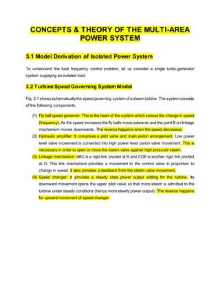
1. CONCEPTS & THEORY OF THE MULTI-AREA
POWER SYSTEM
3.1 Model Derivation of Isolated Power System
To understand the load frequency control problem, let us consider a single turbo-generator
system supplying an isolated load.
3.2 Turbine Speed Governing System Model
Fig. 3.1 shows schematicallythe speed governing system of a steam turbine. The system consists
of the following components.
(1) Fly ball speed governor: This is the heart of the system which senses the change in speed
(frequency). As the speed increases the fly balls move outwards and the point B on linkage
mechanism moves downwards. The reverse happens when the speed decreases.
(2) Hydraulic amplifier: It comprises a pilot valve and main piston arrangement. Low power
level valve movement is converted into high power level piston valve movement. This is
necessary in order to open or close the steam valve against high pressure steam.
(3) Linkage mechanism: ABC is a rigid link pivoted at B and CDE is another rigid link pivoted
at D. This link mechanism provides a movement to the control valve in proportion to
change in speed. It also provides a feedback from the steam valve movement.
(4) Speed changer: It provides a steady state power output setting for the turbine. Its
downward movement opens the upper pilot valve so that more steam is admitted to the
turbine under steady conditions (hence more steady power output). The reverse happens
for upward movement of speed changer.

2. Fig. 3.1 Model of Turbine speed governing system
Let the point A on the linkage mechanism be moved downwards by a small amount ∆yA. It is
a command which causes the turbine power output to change and can therefore be written as
∆yA= KC∆PC (3.1)
Where ∆PC is the commanded increase in power:
The command signal ∆PC (i.e. ∆yE) sets into motion a sequence of events - The pilot valve
moves upwards, high pressure oil flows on to the top of the main piston moving it downwards;
the steam valve opening consequently increases, the turbine generator speed increases, i.e.
the frequency goes up. Let us model these events mathematically.
Two factors contribute to the movement of C:
(1) ∆yA contributes- 2
1
A
L
y
L
 

 
 
or –K1∆yA (i.e. upwards) of 1 C C
K K P
 

3. (2) Increase in frequency ∆f causes the fly balls to move outwards so that B moves
downwards by a proportional amount 2
'
K f
 . The consequent movement of C with A
remaining fixed at ∆yA is 2 2
2 2
1
'
L L
K f K f
L
 

    
 
 
(i. e. downwards)
The net movement of C is therefore
1 2
C C C
y K K P K f
      (3.2)
The movement of D, ∆yD, is the amount by which the pilot valve opens. It is contributed by ∆yC
and ∆yE and can be written as
3
4
3 4 3 4
D C E
L
L
y y y
L L L L
   
    
   
 
   
= K3∆yC+ K4∆yE (3.3)
The movement ∆yD depending upon its sign opens one of the ports of the pilot valve admitting
high pressure oil into the cylinder thereby moving the main piston and opening the steam valve
by ∆yE.
The volume of oil admitted to the cylinder is proportional to the time integral of ∆yD.The movement
∆yE is obtained by dividing the oil volume by the area of the cross section of the piston. Thus
∆yE= 5 0
( )
t
D
k y dt

 (3.4)
Take Laplace transform of Eqs. (3.2), (3.3) and (3.4),
∆YC(s) = -K1KC∆PC(s) + K2∆F(s)
∆YD(s) = -K3∆YC(s) + K4∆YE (s)
5
1
( ) ( )
E D
Y s K Y s
s
 
   
 
 
Eliminating ∆YC(s) and ∆YD(s), we can write

4. 1 3 2 3
4
5
( ) ( )
( ) C C
E
K K K P s K K F s
Y s
s
K
K
  
 
 

 
 
1
( ) ( )
1
sg
C
sg
K
P s F s
R T s
 
 
     
   

   
(3.5)
Where 1
2
C
K K
R
K
 = speed regulation of the governor
1 3
4
C
sg
K K K
K
K
 = gain of speed governor
4 5
1
sg
T
K K
 = time constant of speed governor
The equation can be represented in the form of a block diagram in Fig. 3.2.
Fig. 3.2 Block diagram representation of speed governor system
3.3 Turbine Model
The dynamic response is largely influenced by two factors, (i) entrained steam between the inlet
steam valve and first stage of the turbine, (ii) the storage action in the reheater which causes the
output if the low pressure stage to lag behind that of the high pressure stage. Thus, the turbine
transfer function is characterized by two time constants. For ease of analysis it will be assumed

5. here that the turbine can be modeled to have a single equivalent time constant as given in Fig.
1.3 [19].
Fig. 3.3 Turbine transfer function model
Where, Kt = Gain of turbine, Tt = Time constant of turbine
1.1 Generation-Load Model
For the purposes of AGC synthesis and analysis in the presence of load
disturbances, a simple, low order linearized model is commonly used. The overall
generation-load dynamic relationship between the incremental mismatch power (∆Pm
- ∆PL) and the frequency deviation ∆f can be expressed as
∆𝑃
𝑚(𝑡) − ∆𝑃𝐿(𝑡) = 2𝐻
𝑑∆𝑓(𝑡)
𝑑𝑡
+ 𝐷∆𝑓(𝑡) (3.6)

6. Where ∆𝑃
𝑚 is the mechanical power change, ∆𝑃𝐿 is the load change, H is the inertia
constant, and D is the load damping coefficient and in the laplace transform written
as
∆𝑃
𝑚(𝑠) − ∆𝑃𝐿(𝑠) = 2𝐻𝑠∆𝑓(𝑠) + 𝐷∆𝑓(𝑠) (3.7)
1.11 Area Interface
In a multi area power system, the trend of frequency measured in each control area
is an indicator of trend of the mismatch power in the interconnection and not in the
control area alone. Therefore, the power interchange should be properly considered
in the LFC model. It is easy to show that in an inter-connected power system with N
control area, the tie line power change between area i and other area can be
represented as
∆𝑃𝑡𝑖𝑒,1 = ∆𝑃𝑡𝑖𝑒,12+ ∆𝑃𝑡𝑖𝑒,13 + ∆𝑃𝑡𝑖𝑒,14 + …… …… .. +∆𝑃𝑡𝑖𝑒,1𝑛
∆𝑃𝑡𝑖𝑒,1 =
2𝜋
𝑠
[{𝑇12 + 𝑇13 + 𝑇14 + ⋯… …… …. 𝑇1𝑛}∆𝑓
1 − {𝑇12 + 𝑇13 + 𝑇14 + ⋯…… …… .𝑇1𝑛 }∆𝑓2
∆𝑃𝑡𝑖𝑒,1 =
2𝜋
𝑠
[∑𝑇𝑖𝑗∆𝑓𝑖 −
𝑁
𝑗=1
𝑗≠𝑖
∑𝑇𝑖𝑗∆𝑓
𝑗] (3.8)
𝑁
𝑗=1
𝑗≠𝑖
similarly
∆𝑃𝑡𝑖𝑒,𝑖 = ∑∆𝑃𝑡𝑖𝑒,𝑖𝑗 =
2𝜋
𝑠
𝑁
𝑗=1
𝑗≠𝑖
[∑𝑇𝑖𝑗∆𝑓𝑖 −
𝑁
𝑗=1
𝑗≠𝑖
∑𝑇𝑖𝑗∆𝑓
𝑗] (3.9)
𝑁
𝑗=1
𝑗≠𝑖
Where ∆Pt ie, i indicate the tie line power change of area i and T12 is the synchronizing
torque coefficient between area i and j. The ∆Pt ie, i has been added to the mechanical
power change (∆Pm ) and area load change (∆PL) using an appropriate sign. In
addition to the regulating area frequency, the LFC loop should control the net
interchange power with neighboring areas at scheduled values. This is generally
accomplished by feeding a linear combination of tie-line flow and frequency
deviations, known as area control error (ACE), via supplementary feedback to the
dynamic controller. The ACE can be calculated as

7. ACEi = ∆Pt ie, i + 𝐵i∆fi (3.10)
Where 𝐵i is a bias factor, and its suitable value can be computed as
𝐵𝑖 =
1
𝑅
+ 𝐷𝑖 (3.11)
The effects of local load changes and interface with other areas are also considered
as the following two input signals.
𝑊
1 = ∆𝑃𝐿1 , 𝑊2 = (𝑇21∆𝑓
1 + 𝑇23∆𝑓3 + 𝑇24∆𝑓
4 + ⋯… …… .. +𝑇25∆𝑓5)
𝑊2 = ∑𝑇𝑖𝑗∆𝑓
𝑗 (3.12)
𝑁
𝑗=1
𝑗≠𝑖
Each control area monitors its own tie-line power flow and frequency at the
area control center, and the combined signal (ACE) is allocated to the dynamic
controller. Finally, the resulting control action signal is applied to the turbine-
governor units, according their participation factors.
3.4 Generator LoadModel
The increment in power input to the generator-load system is
∆PG - ∆PD
Where ∆PG = ∆Pt, incremental turbine power output (assuming generator incremental loss to be
negligible) and ∆PD is the load increment.
This increment in power input to the system is accounted for in two ways:
(1) Rate of increase of stored kinetic energy in the generator rotor. At scheduled frequency (fº),
the stored energy is
0
ke r
W H P
 kW = sec (kilojoules)
Where Pr is the kW rating of the turbo-generator and H is defined as its inertia constant.
The kinetic energy being proportional to square of speed (frequency), the kinetic energy at a
frequency of (fº + ∆f) is given by

8. 2
0
0
0
ke ke
f f
W W
f
 
 
  
 
0
2
1
r
f
HP
f
 


 
 
(3.13)
Rate of change of kinetic energy is therefore
  0
2
( )
r
ke
HP
d d
W f
dt f dt
  (3.14)
(ii) As the frequency changes,the motor load changes being sensitive to speed, the rate of change
of load with respect to frequency, i.e. ∂PD/∂f can be regarded as nearly constant for small changes
in frequency ∆f and can be expressed as
D
P
f B f
f
 

  
 

 
(3.15)
Where, the constant B can be determined empirically. B is positive for a predominantly motor
load.
Writing the power balance equation, we have
0
2
( )
r
G D
HP d
P P f B f
f dt
      
Dividing throughout by Pr and rearranging, we get
0
2
( ) ( ) ( ) ( )
G D
H d
P pu P pu f B pu f
f dt
       (3.16)
Taking the Laplace transform, we can write ∆F(s) as
0
( ) ( )
( )
2
G D
P s P s
F s
H
B s
f
  
 


9. = 
( ) ( )
1
G D
Kps
P s P s
TpsS
 
   

 
(3.17)
Where
ps 0
2H
T
Bf
 = power system time constant
ps
1
K
B
 = power system gain
The equation can be represented in block diagram form as in Fig. 3.4
Fig. 3.4 Block diagram representation of generator-load model
3.5 Complete Block Diagram Representation of LFC of an
Isolated Area

10. A complete block diagram representation of an isolated power system comprising turbine,
generator, governor and load is easily obtained by combining the block diagrams (Figs. 3.2, 3.3
and 3.4) with feedback loop as shown in Fig. 3.5
Fig. 3.5 Block Diagram Model of Load Frequency Control
(isolated power system)