SlideShare una empresa de Scribd logo
1 de 41
1. INTRODUCTION
This project deals with the single object tracking and velocity of that
object.
1.1.Motivation
The motivation behind this project is to develop software for tracking, the
major application in security, surveillance and vision analysis. The developed software must
be capable of tracking any single object moving in the frame and to implement on a hardware
which is capable of on board calculations with high performance and low power
consumption. This system might be useful for extending in real-time surveillance or object
classification.
1.2.AIM
Goal of this project is to develop an algorithm for tracking of an object and
determining the velocity of moving object in sequence of frames. All the evaluation has to be
performed on TMS320C6416T DSP starter Kit (DSK), which is capable of doing onboard
calculations. It has features like internal memory and external memory on board to store
instructions and doing evaluation on board. It has special functions for handling graphics up
to ten-times faster then others. Algorithms can be extended for real time applications.
1.3. Outline of the Project
The implementation of object tracking and its velocity determination is
explained stepby step in this report. In chapter 3, few approaches are implemented in real-
time for object tracking and velocity determination are explained. In chapter 5, algorithms
that are developed to accomplish this project are explained. In chapter 6, implementation part
which includes the logical approach of tracking done for the project is described. Inchapter 6,
evaluation part describes the interface between the hardware and workstation, converting the
video into images and loading the images. In chapter 7, results are visualized and
finally concluded.
1
2. DIGITAL IMAGE PROCESSING
2.1BACKGROUND:
Digital image processing is an area characterized by the need for extensive
experimental work to establish the viability of proposed solutions to a given problem. An
important characteristic underlying the design of image processing systems is the significant
level of testing & experimentation that normally is required before arriving at an acceptable
solution. This characteristic implies that the ability to formulate approaches &quickly
prototype candidate solutions generally plays a major role in reducing the cost & time
required to arrive at a viable system implementation.
2.2. What is DIP?
An image may be defined as a two-dimensional function f(x, y), where x & y are
spatial coordinates,& the amplitude of f at any pair of coordinates (x, y) is called the
intensity or gray level of the image at that point. When x, y & the amplitude values of f
are all finite discrete quantities, we call the image a digital image. The field of DIP refers
to processing digital image by means of digital computer. Digital image is composed of a
finite number of elements, each of which has a particular location & value. The elements
are called pixels.
Vision is the most advanced of our sensor, so it is not surprising that image play
the single most important role in human perception. However, unlike humans, who are
limited to the visual band of the EM spectrum imaging machines cover almost the entire EM
spectrum, ranging from gamma to radio waves. They can operate also on images generated
by sources that humans are not accustomed to associating with image.
There is no general agreement among authors regarding where image processing
stops & other related areas such as image analysis& computer vision start. Sometimes a
distinction is made by defining image processing as a discipline in which both the input &
output at a process are images. This is limiting & somewhat artificial boundary. The area of
image analysis (image understanding) is in between image processing & computer vision.
There are no clear-cut boundaries in the continuum from image processing at one end
to complete vision at the other. However, one useful paradigm is to consider three types of
2
computerized processes in this continuum: low,mid & high-level processes. Low-level
process involves primitive operations such as image processing to reduce noise, contrast
enhancement & image sharpening. A low- level process is characterized by the fact that both
its inputs & outputs are images. Mid-level process on images involves tasks such as
segmentation, description of that object to reduce them to a form suitable for computer
processing & classification of individual objects. A mid-level process is characterized by the
fact that its inputs generally are images but its outputs are attributes extracted from those
images. Finally higher-level processing involves“Making sense”of an ensemble of recognized
objects, as in image analysis & at the far end of the continuum performing the cognitive
functions normally associated with human vision.
Digital image processing, as already defined is used successfully in a broad range of
areas of exceptional social & economic value.
2.3.Gray scale image:
A grayscale image is a function I(x,y) of the two spatial
coordinates of the image plane. I(x, y) is the intensity of the image at the point (x, y) on the
image plane.
2.4.Color image:
It can be represented by three functions, R(x,y) for red, G(x,y) for
green and B (x,y) for blue.An image may be continuous with respect to the x and y
coordinates and also in amplitude. Converting such an image to digital form requires that the
coordinates as well as the amplitude to be digitized. Digitizing the coordinate’s values is
called sampling. Digitizing the amplitude values is called quantization.
3
2.5.Coordinate convention:
The result of sampling and quantization is a matrix of real numbers. We use two
principal ways to represent digital images. Assume that an image f(x, y) is sampled so that
the resulting image has M rows and N columns. We say that the image is of size M X N. The
values of the coordinates (x,y) are discrete quantities. For notational clarity and convenience,
we use integer values for these discrete coordinates. In many image processing books, the
image origin is defined to be at (x,y)=(0,0).The next coordinate values along the first row of
the image are (x,y)=(0,1).It is important to keep in mind that the notation (0,1) is used to
signify the second sample along the first row. It does not mean that these are the actual
values of physical coordinates when the image was sampled. Following figure shows the
coordinate convention. Note that x ranges from 0 to M-1 and y from 0 to N-1 in integer
increments.
The coordinate convention used in the toolbox to denote arrays is different from the
preceding paragraph in two minor ways. First, instead of using (x,y) the toolbox uses the
notation (race) to indicate rows and columns. Note, however, that the order of coordinates is
the same as the order discussed in the previous paragraph, in the sense that the first element
of a coordinate topples, (a,b) refers to a row and the second to a column. The other difference
is that the origin of the coordinate system is at (r, c) = (1, 1); thus, r ranges from 1 to M and c
from 1 to N in integer increments. IPT documentation refers to the coordinates. Less
frequently the toolbox also employs another coordinate convention called spatial coordinates
which uses x to refer to columns and y to refers to rows. This is the opposite of our use of
variables x and y.
2.6.Image as Matrices:
The preceding discussion leads to the following representation for a digitized image
function: f (0,0) f(0,1) ……….. f(0,N-1)
f(1,0) f(1,1) ………… f(1,N-1)
f(x,y)= . . .
f(M-1,0) f(M-1,1) ………… f(M-1,N-1)
4
The right side of this equation is a digital image by definition. Each element of
this array is called an image element, picture element, pixel or pel. The terms image and pixel
are used throughout the rest of our discussions to denote a digital image and its elements.
A digital image can be represented naturally as a MATLAB matrix:
f(1,1) f(1,2) ……. f(1,N)
f(2,1) f(2,2) …….. f(2,N)
f = . . .
. . .
f(M,1) f(M,2) …….f(M,N)
Where f(1,1) = f(0,0) (note the use of a monoscope font to
denote MATLAB quantities). Clearly the two representations are identical, except for the
shift in origin. The notation f(p,q) denotes the element located in row p and the column q.
For example f(6,2) is the element in the sixth row and second column of the matrix f.
Typically we use the letters M and N respectively to denote the number of rows and columns
in a matrix. A 1xN matrix is called a row vector whereas an Mx1 matrix is called a column
vector. A 1x1 matrix is a scalar.
Matrices in MATLAB are stored in variables with names such as A, a, RGB, real array
and so on. Variables must begin with a letter and contain only letters, numerals and
underscores. As noted in the previous paragraph, all MATLAB quantities are written using
mono-scope characters. We use conventional Roman, italic notation such as f(x,y) for
mathematical expressions.
3.SINGLE OBJECT TRACKING
5
Object tracking is the process of locating and following the moving object in
sequence of video frames. Smart cameras are used as input sensors to record the video. The
recorded video may have some noise due to bad weather (light, wind, etc. or due to problems
in sensors). Few algorithms are tested to improve the image quality, to detect moving object,
calculation of distance and velocity of the moving object.
3.1. Pre-processing
The pre-processing performs some steps to improve the image quality. Few
algorithms are explained and filtering is done by using box-filter techniques. Box
functionality .If we take an image with X*Y resolution, the pixels starting from 2nd row 2nd
column to X-1 row Y-1 column are scanned with all the neighbouring elements, they form a
shape like box. The pixels from 2nd row 2nd column to X-1 row Y-1column are taken into
consideration since we need to scan all the surrounding elements and for the 1st row ,1st
column, last row and last column elements are not possible to scan there surrounding
elements as they don't have.
3.1.1. Mean Filter
Mean filter is the simplest type of low pass filter to remove noise. The noise is removed
using the box functionality, which scans the whole image. For every pixel the mean from
the box elements are calculated and the pixel values are stored in to the central element.
Let us consider an example with 3x3 matrixes
1 2 9
4 3 8
5 6 7
Pixel:value = (1 + 2 + 3 + 4 + 5 + 6 + 7 + 8 + 9)/9
in the above matrix, central element is '3' and after calculating the pixel value, the value of 5
SINGLE OBJECT TRACKING 3
3 is replaced by the pixel value. The calculation time for mean filter is very less compared to
all other. By using this filter smoothing is done.
3.1.2. Gaussian Smoothing
Gaussian smoothing operator is used to blur images and remove noise. Gaussian
smoothing has the similarity of mean filter, but uses a different function to calculate the pixel
value.
6
A box is scanned over the whole image and the pixel value calculated from the standard
deviation of Gaussian is stored in the central element. The size of the box may vary from 1 to
7 means 1x1 to 7x7 elements.
3.1.3.Median Filter
The median filter is a classical noise removal filter. Noise is removed by calculating
the median from all its box elements and stores the value to the central element. If we
consider and example of 3x3 matrix
1 2 9
4 3 8
5 6 7
The median filter sorts the elements in a given matrix and median value is assigned tothe
central pixel. Sorted elements 1, 2, 3, 4, 5, 6, 7, 8, 9 and median 5 will assign to the central
element. Similar box scan is performed over the whole image and reduces noise. Execution
time is more compared to mean filter, since the algorithm involves with sorting techniques.
But it removes the small pixel noise.
3.2. Segmentation
Segmentation is the process of dividing digital image into multiple regions.
Segmentation shows the objects and boundaries in an image. Each Pixel in the region has
some similarcharacteristics like colour, intensity, etc. Few methods for segmenting the
images are explained below.
3.2.1. Histogram Based Segmentation
One of the simple ways of doing segmentation is using histogram. Histogram is
computedfor all the image pixels. The peaks in histogram are produced by the intensity
values that are produced after applying the threshold and clustering. The pixel value is used
to locate the regions in the image. Based on histogram values and threshold we can classify
the low intensity values as object and the high values are background image (most of the
cases).
3.2.2. Single Gaussian Background Method
Single gaussian background model is used to separate the background and
foregroundobjects. It is a statically method of separation. In this a set of frames (previous
frames) are taken and the calculation is done for separation. The separation is performed by
calculating the mean and variance at each pixel position.
7
3.2.3. Frame Difference
Frame difference calculates the difference between 2 frames at every pixel position
and store the absolute difference. It is used to visualize the moving objects in a sequence of
frames. It takes very less memory for performing the calculation.
Let us consider an example, if we take a sequence of frames, the present frame
and the next frame are taken into consideration at every calculation and the frames are shifted
(after calculation the next frame becomes present frame and the frame that comes in sequence
becomes next frame).
3.3. Feature Extraction
Feature Extraction plays a major role to detect the moving objects in sequence of
frames .Every object has a specific feature like colour or shape. In a sequence of frames, any
one of the feature is used to detect the objects in the frame.
3.3.1. Edges
Edges are formed where there is a sharp change in the intensity of images. If there is
an object, the pixel positions of the object boundary are stored and in the next sequence of
frames this position is verified. Corner based algorithm uses the pixel position of edges for
defining and tracking of objects
3.3.2. Bounding Box with Colour Feature
If the segmentation is performed using frame difference, the residual image is
visualizedwith rectangular bounding box with the dimensions of the object produced from
residualimage. For a given image, a scan is performed where the intensity values of the image
is more then limit (depends on the assigned value, for accurate assign maximum). In this
Features is extracted by colour and here the intensity value describes the colour. The pixel
values from the first hit of the intensity values from top, bottom, left and right are stored. By
using this dimension values a rectangular bounding box is plotted within the limits of the
values produced.
3.4. Object Detection
Extraction of objects using the features is known as object detection. Every object
has a specific feature based on its dimensions. Applying feature extraction algorithm, the
object in each frame can be pointed out.
3.4.1. Optical Flow
Optical flow is one way to detect moving objects in a sequence of frames. In this, the
8
vector position of pixels is calculated and compared in sequence of frames for the pixel
position. Typically the motion is represented as vector position of pixels.
3.4.2. Block Matching
Block matching algorithm is a standard technique for determining the moving object in
video. Blocks are formed in a region without overlapping on the other region. Every block in
a frame is compared to the corresponding blocks in the sequence of frames and compares the
smallest distance of pixel values.
3.5. Tracking
The process of locating the moving object in sequence of frames is known as tracking.
This tracking can be performed by using the feature extraction of objects and detecting
the objects in sequence of frames. By using the position values of object in every frame,
we can calculate the position and velocity of the moving object.
3.5.1. Velocity
The velocity of moving object is calculated by the distance it travelled with respect
to the time. Euclidean distance formula is used to calculate the distance between the
sequences of frames. By using the values of distance with respect to frame rate, the velocity
of the object is defined. The defined velocity is of 2-dimension (since camera is static).
4. MAT LAB
4.1. What is MATLAB
MATLAB is a high-level technical computing language and interactive
environment for algorithm development, data visualization, data analysis, and numeric
9
computation. Using the MATLAB product, you can solve technical computing problems
faster than with traditional programming languages, such as C, C++, and Fortran.
You can use MATLAB in a wide range of applications, including signal
and image processing, communications, control design, test and measurement, financial
modeling and analysis, and computational biology. Add-on toolboxes (collections of special-
purpose MATLAB functions, available separately) extend the MATLAB environment to
solve particular classes of problems in these application areas.
MATLAB provides a number of features for documenting and sharing your work. You can
integrate your MATLAB code with other languages and applications, and distribute your
MATLAB algorithms and applications.
4.2. Key Features
• High-level language for technical computing.
• Development environment for managing code, files, and data.
• Interactive tools for iterative exploration, design, and problem solving.
• Mathematical functions for linear algebra, statistics, Fourier analysis, filtering,
optimization, and numerical integration.
• 2-D and 3-D graphics functions for visualizing data.
• Tools for building custom graphical user interfaces.
• Functions for integrating MATLAB based algorithms with external applications and
languages, such as C, C++, Fortran, Java, COM, and Microsoft Excel.
4.3. Developing Algorithms and Applications
MATLAB provides a high-level language and development tools that let you quickly
develop and analyze your algorithms and applications.
4.4. The MATLAB Language
The MATLAB language supports the vector and matrix operations that are
fundamental to engineering and scientific problems. It enables fast development and
execution.
With the MATLAB language, you can program and develop algorithms faster
10
than with traditional languages because you do not need to perform low-level administrative
tasks, such as declaring variables, specifying data types, and allocating memory. In many
cases, MATLAB eliminates the need for ‘for’ loops. As a result, one line of MATLAB code
can often replace several lines of C or C++ code.
At the same time, MATLAB provides all the features of a traditional
programming language, including arithmetic operators, flow control, data structures, data
types, object-oriented programming (OOP), and debugging features.
4.5. Analyzing and Accessing Data
MATLAB supports the entire data analysis process, from acquiring data from
External devices and databases, through preprocessing, visualization, and numerical analysis,
to producing presentation-quality output.
4.5.1. Data Analysis
The MATLAB product provides interactive tools and command-line functions for
data analysis operations, including:
• Interpolating and decimating.
• Extracting sections of data, scaling, and averaging.
• Thresholding and smoothing.
• Correlation, Fourier analysis, and filtering.
• 1-D peak, valley, and zero finding.
• Basic statistics and curve fitting.
• Matrix analysis.
4.5.2.Dataaccess
MATLAB is an efficient platform for accessing data from files, other applications, databases,
and external devices. You can read data from popular file formats, such as Microsoft Excel;
ASCII text or binary files; image, sound, and video files
4.6. Publishing Results and Deploying Applications
11
MATLAB provides a number of features for documenting and sharing your work.
You can integrate your MATLAB code with other languages and applications and deploy
your MATLAB algorithms and applications as stand-alone programs or software modules.
4.6.1. Publishing Results
The MATLAB product lets you export your results as plots or as complete reports.
You can export plots to all popular graphics file formats and then import the plots into other
packages, such as Microsoft Word or Microsoft PowerPoint. Using the MATLAB Editor, you
can automatically publish your MATLAB code in HTML, Word, LATEX, and other formats.
MATLAB program (left) published to HTML (right) using the MATLAB Editor.
Results output to the command window or to plots are captured and included, and the
comments are turned into section headings and body text in the HTML.
To create more complex reports, such as simulation runs and multiple parameter
tests, you can use the MATLAB Report Generator (available separately).
4.6.2. Integrating MATLAB Code with Other Languages and Applications
MATLAB provides functions for integrating C and C++ code, Fortran code, COM
objects, and Java code with your applications. You can call DLLs, Java classes, and ActiveX
controls. Using the MATLAB engine library, you can also call MATLAB from C, C++, or
Fortran code.
4.6.3. Deploying Applications
You can create your algorithm in MATLAB and distribute it to other MATLAB
users directly as MATLAB code. Using the MATLAB Compiler (available separately), you
can deploy your algorithm, as a stand-alone application or as a software module that you
include in your project, to users who do not have MATLAB.
4.7. Reading Images
Images are read into the MATLAB environment using function imread whose
syntax is imread(‘filename’)
Format name Description Recognized extension
TIFF Tagged Image File Format .tif, .tiff
12
JPEG Joint Photograph Experts Group .jpg, .jpeg
GIF Graphics Interchange Format .gif
BMP Windows Bitmap .bmp
PNG Portable Network Graphics .png
XWD X Window Dump .xwd
Here filename is a spring containing the complete of the image file(including any
applicable extension).For example the command line
>> f = imread (‘8. jpg’);
reads the JPEG (above table) image chestXray into image array f. Note the use of single
quotes (‘) to delimit the string filename. The semicolon at the end of a command line is used
by MATLAB for suppressing output. If a semicolon is not included. MATLAB displays the
results of the operation(s) specified in that line. The prompt symbol(>>) designates the
beginning of a command line, as it appears in the MATLAB command window.
When as in the preceding command line no path is included in filename, imread reads
the file from the current directory and if that fails it tries to find the file in the MATLAB
search path. The simplest way to read an image from a specified directory is to include a full
or relative path to that directory in filename.
For example,
>> f = imread ( ‘D:myimageschestxray.jpg’);
reads the image from a folder called my images on the D: drive, whereas
>> f = imread(‘ .  myimageschestxray .jpg’);
reads the image from the my images subdirectory of the current of the current working
directory. The current directory window on the MATLAB desktop toolbar displays
MATLAB’s current working directory and provides a simple, manual way to change it.
Above table lists some of the most of the popular image/graphics formats supported by
imread and imwrite.
13
Function size gives the row and column dimensions of an image:
>> size (f)
ans = 1024 * 1024
This function is particularly useful in programming when used in the following form to
determine automatically the size of an image:
>>[M,N]=size(f);
This syntax returns the number of rows(M) and columns(N) in the image.
The whole function displays additional information about an array. For instance ,the
statement
>> whos f
gives
Name size Bytes Class
F 1024*1024 1048576 unit8 array
Grand total is 1048576 elements using 1048576 bytes
The unit8 entry shown refers to one of several MATLAB data classes. A semicolon at
the end of a whose line has no effect ,so normally one is not used.
4.8. Displaying Images:
Images are displayed on the MATLAB desktop using function imshow, which has the
basic syntax:
imshow(f, g)
Where f is an image array, and g is the number of intensity levels used to display
it. If g is omitted ,it defaults to 256 levels .using the syntax
14
imshow(f,{low high})
Displays as black all values less than or equal to low and as white all values
greater than or equal to high. The values in between are displayed as intermediate intensity
values using the default number of levels .Finally the syntax
Imshow(f,[ ])
Sets variable low to the minimum value of array f and high to its maximum value.
This form of imshow is useful for displaying images that have a low dynamic range or that
have positive and negative values.
Function pixval is used frequently to display the intensity values of individual pixels
interactively. This function displays a cursor overlaid on an image. As the cursor is moved
over the image with the mouse the coordinates of the cursor position and the corresponding
intensity values are shown on a display that appears below the figure window .When working
with color images, the coordinates as well as the red, green and blue components are
displayed. If the left button on the mouse is clicked and then held pressed, pixval displays the
Euclidean distance between the initial and current cursor locations.
The syntax form of interest here is Pixval which shows the cursor on the last image
displayed. Clicking the X button on the cursor window turns it off.
The following statements read from disk an image called rose_512.tif extract basic
information about the image and display it using imshow :
>>f=imread(‘rose_512.tif’);
>>whos f
Name Size Bytes Class
F 512*512 262144 unit8 array
Grand total is 262144 elements using 262144 bytes
>>imshow(f)
15
A semicolon at the end of an imshow line has no effect, so normally one is not used.
If another image,g, is displayed using imshow, MATLAB replaces the image in the screen
with the new image. To keep the first image and output a second image, we use function
figure as follows:
>>figure , imshow(g)
Using the statement
>>imshow(f),figure ,imshow(g) displays both images.
Note that more than one command can be written on a line ,as long as
different commands are properly delimited by commas or semicolons. As mentioned earlier,
a semicolon is used whenever it is desired to suppress screen outputs from a command line.
Suppose that we have just read an image h and find that using imshow produces the image. It
is clear that this image has a low dynamic range, which can be remedied for display purposes
by using the statement.
>>imshow(h,[ ])
4.9. WRITING IMAGES:
Images are written to disk using function imwrite, which has the following basic syntax:
Imwrite (f,’filename’)
With this syntax, the string contained in filename must include a recognized file format
extension .Alternatively, the desired format can be specified explicitly with a third input
argument. >>imwrite(f,’patient10_run1’,’tif’)
Or alternatively
For example the following command writes f to a TIFF file named patient10_run1:
16
>>imwrite(f,’patient10_run1.tif’)
If filename contains no path information, then imwrite saves the file
in the current working directory.
The imwrite function can have other parameters depending on e file format selected.
Most of the work in the following deals either with JPEG or TIFF images ,so we focus
attention here on these two formats. More general imwrite syntax applicable only to
JPEG images is
imwrite(f,’filename.jpg,,’quality’,q)
where q is an integer between 0 and 100(the lower number the higher the degradation due to
JPEG compression).
For example, for q=25 the applicable syntax is
>> imwrite(f,’bubbles25.jpg’,’quality’,25)
The image for q=15 has false contouring that is barely visible, but this effect becomes
quite pronounced for q=5 and q=0.Thus, an expectable solution with some margin for error is
to compress the images with q=25.In order to get an idea of the compression achieved and to
obtain other image file details, we can use function imfinfo which has syntax.
Imfinfo filename
Here filename is the complete file name of the image stored in disk.
For example,
>> imfinfo bubbles25.jpg
outputs the following information(note that some fields contain no information in this
case):
Filename: ‘bubbles25.jpg’
FileModDate: ’04-jan-2003 12:31:26’
17
FileSize: 13849
Format: ‘jpg’
Format Version: ‘ ‘
Width: 714
Height: 682
Bit Depth: 8
Color Depth: ‘grayscale’
Format Signature: ‘ ‘
Comment: { }
Where file size is in bytes. The number of bytes in the original image is corrupted
simply by multiplying width by height by bit depth and dividing the result by 8. The result is
486948.Dividing this file size gives the compression ratio:(486948/13849)=35.16.This
compression ratio was achieved. While maintaining image quality consistent with the
requirements of the appearance. In addition to the obvious advantages in storage space, this
reduction allows the transmission of approximately 35 times the amount of un compressed
data per unit time.
The information fields displayed by imfinfo can be captured in to a so called structure
variable that can be for subsequent computations. Using the receding an example and
assigning the name K to the structure variable.
We use the syntax >>K=imfinfo(‘bubbles25.jpg’);
To store in to variable K all the information generated by command imfinfo, the
information generated by imfinfo is appended to the structure variable by means of fields,
separated from K by a dot. For example, the image height and width are now stored in
structure fields K. Height and K. width.
18
As an illustration, consider the following use of structure variable K to commute the
compression ratio for bubbles25.jpg:
>> K=imfinfo(‘bubbles25.jpg’);
>> image_ bytes =K.Width* K.Height* K.Bit Depth /8;
>> Compressed_ bytes = K.FilesSize;
>> Compression_ ratio=35.162
Note that iminfo was used in two different ways. The first was t type imfinfo
bubbles25.jpg at the prompt, which resulted in the information being displayed on the screen.
The second was to type K=imfinfo (‘bubbles25.jpg’),which resulted in the information
generated by imfinfo being stored in K. These two different ways of calling imfinfo are an
example of command_ function duality, an important concept that is explained in more detail
in the MATLAB online documentation.
More general imwrite syntax applicable only to tif images has the form
Imwrite(g,’filename.tif’,’compression’,’parameter’,….’resloution’,[colres rowers] )
Where ‘parameter’ can have one of the following principal values: ‘none’ indicates no
compression, ‘pack bits’ indicates pack bits compression (the default for non ‘binary
images’) and ‘ccitt’ indicates ccitt compression. (the default for binary images).The 1*2 array
[colres rowers]
Contains two integers that give the column resolution and row resolution in dot per_
unit (the default values). For example, if the image dimensions are in inches, colres is in the
number of dots(pixels)per inch (dpi) in the vertical direction and similarly for rowers in the
horizontal direction. Specifying the resolution by single scalar, res is equivalent to writing
[res res].
>>imwrite(f,’sf.tif’,’compression’,’none’,’resolution’,……………..[300 300])
the values of the vector[colures rows] were determined by multiplying 200 dpi by the ratio
2.25/1.5, which gives 30 dpi. Rather than do the computation manually, we could write
19
>> res=round(200*2.25/1.5);
>>imwrite(f,’sf.tif’,’compression’,’none’,’resolution’,res)
where its argument to the nearest integer.It function round rounds is important to note
that the number of pixels was not changed by these commands. Only the scale of the image
changed. The original 450*450 image at 200 dpi is of size 2.25*2.25 inches. The new
300_dpi image is identical, except that is 450*450 pixels are distributed over a 1.5*1.5_inch
area. Processes such as this are useful for controlling the size of an image in a printed
document without sacrificing resolution.
Often it is necessary to export images to disk the way they appear on the MATLAB
desktop. This is especially true with plots .The contents of a figure window can be exported
to disk in two ways. The first is to use the file pull-down menu is in the figure window and
then choose export. With this option the user can select a location, filename, and format.
More control over export parameters is obtained by using print command:
Print-fno-dfileformat-rresno filename
Where no refers to the figure number in the figure window interest, file format
refers one of the file formats in table above. ‘resno’ is the resolution in dpi, and filename is
the name we wish to assign the file.
If we simply type print at the prompt, MATLAB prints (to the default printer) the
contents of the last figure window displayed. It is possible also to specify other options with
print, such as specific printing device.
4.10. Data Classes:
Although we work with integers coordinates the values of pixels themselves are not
restricted to be integers in MATLAB. Table above list various data classes supported by
MATLAB and IPT are representing pixels values. The first eight entries in the table are refers
to as numeric data classes. The ninth entry is the char class and, as shown, the last entry is
referred to as logical data class.
20
All numeric computations in MATLAB are done in double quantities, so this is also a
frequent data class encounter in image processing applications.Class unit 8 also is
encountered frequently, especially when reading data from storages devices, as 8 bit images
are most common representations found in practice. These two data classes, classes logical,
and, to a lesser degree, class unit 16 constitute the primary data classes on which we focus.
Many ipt functions however support all the data classes listed in table. Data class double
requires 8 bytes to represent a number uint8 and int 8 require one byte each, uint16 and int16
requires 2bytes and unit 32.
Name Description
Double Double _ precision, floating_ point numbers the Approximate.
Uinit8 unsigned 8_bit integers in the range [0,255]
(1byte per element).
Uinit16 unsigned 16_bit integers in the range [0,65535]
(2byte per element)
Uinit 32 unsigned 32_bit integers in the range [0,4294967295]
(4 bytes per element).
Int8 signed 8_bit integers in the range[-128,127]
(1 byte per element)
Int 16 signed 16_byte integers in the range [32768, 32767]
(2 bytes per element).
Int 32 Signed 32_byte integers in the range [-2147483648, 21474833647]
(4 byte per element).
21
Single single _precision floating _point numbers with values
In the approximate range (4 bytes per elements).
Char characters (2 bytes per elements).
Logical values are 0 to 1 (1byte per element).
int 32 and single, required 4 bytes each. The char data class holds characters in Unicode
representation. A character string is merely a 1*n array of characters logical array contains
only the values 0 to 1,with each element being stored in memory using function logical or by
using relational operators.
Image Types:
The toolbox supports four types of images:
1 .Intensity images
2. Binary images
3. Indexed images
4. R G B images
Most monochrome image processing operations are carried out using binary or
intensity images, so our initial focus is on these two image types. Indexed and RGB colour
images.
4.11. Intensity Images:
An intensity image is a data matrix whose values have been scaled to represent
intentions. When the elements of an intensity image are of class unit8, or class unit 16, they
have integer values in the range [0,255] and [0, 65535], respectively. If the image is of class
double, the values are floating _point numbers. Values of scaled, double intensity images are
in the range [0, 1] by convention.
4.12. Binary Images:
Binary images have a very specific meaning in MATLAB.A binary image is a logical
array 0s and1s.Thus, an array of 0s and 1s whose values are of data class, say unit8, is not
22
considered as a binary image in MATLAB .A numeric array is converted to binary using
function logical. Thus, if A is a numeric array consisting of 0s and 1s, we create an array B
using the statement.
B=logical (A)
If A contains elements other than 0s and 1s.Use of the logical function converts all
nonzero quantities to logical 1s and all entries with value 0 to logical 0s.
Using relational and logical operators also creates logical arrays.
To test if an array is logical we use the I logical function:
islogical(c)
If c is a logical array, this function returns a 1.Otherwise returns a 0. Logical array can
be converted to numeric arrays using the data class conversion functions.
4.13. Indexed Images:
An indexed image has two components:
• A data matrix integer, x.
• A color map matrix, map.
Matrix map is an m*3 arrays of class double containing floating_ point values in the
range [0, 1].The length m of the map are equal to the number of colors it defines. Each row of
map specifies the red, green and blue components of a single color. An indexed images uses
“direct mapping” of pixel intensity values color map values. The color of each pixel is
determined by using the corresponding value the integer matrix x as a pointer in to map. If x
is of class double ,then all of its components with values less than or equal to 1 point to the
first row in map, all components with value 2 point to the second row and so on. If x is of
class units or unit 16, then all components value 0 point to the first row in map, all
components with value 1 point to the second and so on.
4.14. RGB Image:
An RGB color image is an M*N*3 array of color pixels where each color pixel
is triplet corresponding to the red, green and blue components of an RGB image, at a specific
23
spatial location. An RGB image may be viewed as “stack” of three gray scale images that
when fed in to the red, green and blue inputs of a color monitor.Produce a color image on the
screen. Convention the three images forming an RGB color image are referred to as the red,
green and blue components images. The data class of the components images determines
their range of values. If an RGB image is of class double the range of values is [0, 1].
Similarly the range of values is [0,255] or [0, 65535].For RGB images of class
units or unit 16 respectively. The number of bits use to represents the pixel values of the
component images determines the bit depth of an RGB image. For example, if each
component image is an 8bit image, the corresponding RGB image is said to be 24 bits deep.
Generally, the number of bits in all component images is the same. In this case the number of
possible color in an RGB image is (2^b) ^3, where b is a number of bits in each component
image. For the 8bit case the number is 16,777,216 colors video into images and loading the
images. In chapter 6, results are visualized and finally concluded.
5. ALGORITHMS
This chapter explains the algorithms to track the single object and to estimate the
velocity of moving object. The sequential approach to track the moving objects and the
velocity of objects are as follow.
• Noise removal: To improve the image quality
• Segmentation: To separate multiple regions in image
• Feature Extraction: To analyze the regions in image
• Tracking : Analyzing the position, velocity and moving direction of object
5.1. Noise removal
A noise removal algorithm is developed by using the median filter as explained in section
4.1.3. Algorithm for noise removal is explained as follow
1. Read the input image
2. for (present position=initial position: final position)
(a) Scan all the surrounding elements
(b) Use bubble sort technique to sort all the values
(c) Calculate the median of it
3. Assign the value to the 'present position' of the input image
24
initial position = 2nd row, 2nd column of an image resolution
final position = (n-1) row, (n-1) column of an image resolution
present position = the pixel value and it varies from initial to final position
Values are taken from 2nd row-2nd column to (n-1) row-(n-1) column because we need to
scan all the surrounding elements of each pixel.
5.2. Segmentation
To perform the segmentation operation, frame difference algorithm is implemented as it takes
less processing time. Frame difference algorithm performs separation of two
sequential frames and it is explained in detail in section 4.2.3. Algorithm for the segmentation
is explained as follow
1. Read the input images
2. for (present position=initial position: final position)
(a) Difference between the pixels values at present position of two images is calculated
(b) Calculate the absolute value
(c) Store the difference in new image at same pixel position that is at present position
5.3. Feature Extraction
Every object has a specific feature which is used to visualize the object and used for
tracking. After performing the segmentation, a rectangular bounding box is plotted with
the dimensions of the object produced in the residual image. Section 4.3.2 explains a clear
view on bounding box. Algorithm for the bounding box is as followed
1. Read the image difference
2. for (present position=initial value: final value) of Y resolution
3. for (present position=initial value: final value) of X resolution
(a) calculate the sharp change in intensity of image from top and bottom
(b) store the values in an array
4. Height of the bounding box is = bottom value- top value
5. for (present position=initial value: final value) of X resolution
6. for (present position=initial value: final value) of Y resolution
(a) calculate the sharp change in intensity of image from left and right
(b) store the values in an array
7. Width of the bound box = right value - left value
8. Using the dimensions, draw boundary to the image
Initial value: the starting position of the pixel in an image. Final value: the ending
25
position of the pixel in an image.
Height = bottom:value / top:value
Width = right:value /left:value
9. Add the height value with the top value and store it in a variable like mid top
10. Add the width value to the left value and store it in a variable like mid left
11. Assign the max intensity to the pixel at pixel value at (mid top, mid left)
5.4. Distance
The distance travelled by the object is determined by using the centroid. It is calculated
by using the Euclidean distance formula. The variables for this are the pixel positions of
the moving object at initial stage to the final stage. Algorithm for calculating distance is
explained as follow
1. Read the centroid position of each image.
2. Calculate the distance between two centroid images
3. for (present position=initial value: final value) of X resolution
4. for (present position=initial value: final value) of Y resolution
5. Calculate change in distance by
Distance=(X2 /X1)2 + (Y 2 /Y 1)2
Where X1=previous pixel position and X2=present pixel position in width
Y1=previous pixel position and Y2=present pixel position in height
6. Store all the distance values in an Array.
5.5.Velocity
Velocity of moving object is determined using the distance travelled by the centroid to the
frame rate of the video. Section 2.5.1 explains the velocity in 2-dimension. Algorithm for
calculating velocity is explained as follow
1. Read the distance travelled by the object
2. Velocity = distance:travelled/ frame:rate
3. Save the value in an array
4. The velocity of moving object in the sequence frames is defined in pixels / second
26
6. IMPLEMENTATION & EVALUTION
This chapter explains the implementation and evaluation of algorithms for single
object tracking. Algorithms for the single object tracking are developed in C language and
evaluated on TMS320C6416T DSP Starter Kit (DSK). The task is performed by recording a
video using digital camera with 30fps. The implementation is initially performed on matlab
and various methods for object tracking are tested. Among the tested methods, frame
difference is used for further calculations, since it satisfies the available conditions (execution
time and memory) of hardware. The initial steps before object tracking include video to
image conversion, images to input format of the TMS320C6416T. The algorithms that are
created are deployed into MATLAB/SIMULATION by using the code composer studio.
27
Fig: 6.1.Block Diagram Of Video Tracking
6.1. Hardware Specification
MATLAB/SIMULATION is a low-cost standalone development platform that enables users
to evaluate and develop applications for C64XX DSP family. It is the Highest-Performance.
Fixed-Point Digital Signal Processors (DSPs) with Advanced Very-Long-Instruction-Word
(VLIW). The DSK also serves as a hardware reference design for the TMS320C6416T DSP.
The DSP on the 6416T DSK interfaces to on-board peripherals through one of two busses;
there are 2 external memories with 64-bit wide External Memory Interface Function A
(EMIFA) and the 8-bit wide External Memory Interface Function B (EMIFB). The SDRAM,
Flash and CPLD are each connected to one of the busses. EMIFA is also connected to the
daughter card expansion connectors which are used for third party add-in boards. Each EMIF
(External Memory Interface) has 4 separate addressable regions called chip enable spaces
28
(CE0-CE3). The SDRAM occupies CE0 of EMIFA while the CPLD and Flash are mapped to
CE0 and CE1 of EMIFB respectively. Daughter cards use CE2 and CE3 of EMIFA. It is
operated at 1 Gigahertz frequency and has 16 Mbytes of synchronous DRAM and 512 Kbytes
of non-volatile Flash memory. Code composer studio software is used as interface between
the TMS320C6416T DSP starter kit (DSK) and the workstation (computer). The input data
must be in hexadecimal format for the code composer studio. Code Composer communicates
with the DSK through an embedded Joint Test Action Group (JTAG) emulator with a USB
host interface. The DSK can also be used with an external emulator through the external
JTAG connector.
From the available hardware memory, SDRAM memory is used for storing the input images,
temporary images and the final output images. The starting address of the SDRAM is from
0x80000000 and the available space is till 0x90000000.
6.2. Conversion
Conversion explains the functions that are performed to convert the recorded video into
input format of image to code composer studio. The steps for the conversion are
• Video to images
• Images to hexadecimal format
6.2.1. Video to images
The task of object tracking is performed by a video recorded with digital camera. The
recorded video is in format of .mov with 30 fps. The video is converted into .avi format
with 20 fps using ULEAD VIDEO STUDIO 10.0 [3]. The frame rate of the video is
converted to
• reduce the frame size of video clip as we can see all the actions in less frames
• less memory can be used for calculations
• change in position of object can be easily observed in each frame
The converted video frames is now spitted into individual frames and converted each into
jpg image format using Image Video Machine 3.2 software.
6.2.2. Image to hexadecimal format
The images are converted into hexadecimal format by using a simple C language program.
This program takes pgm format images as input and converts it into hexadecimal. The initial
condition, we convert the available images into pgm format, it is done by using GIMP
software [1] which converts jpg format to pgm format). After converting the image to pgm
29
format, C program is executed for each image and exported to hexadecimal format of the
image. Algorithm of the C program used for conversion is explained as follow
1. Read the input image
2. Create a temporary array to store the image data
3. Create a file to store the output image
4. while (end of pixel values)
(a) Convert the pixel value into hexadecimal value and store them in temporary
created array
(b) for (every 4 pixel values)
• Store the hexadecimal values in the output file in reverse order.
• Shift to new line
In this, hexadecimal values are stored in row and is shifted to new line after 4 bits.
The output image is imported into code composer studio by assigning the starting address
of it. This starting address is used as input reference for the implementation part.
Ex: The starting address of the input image is 0x80000000 (Address I used in
implementation) in code composer studio.
6.3. Problems
The problems that are faced during the evaluation part are
• Memory : Out of memory error, during execution. Due to overlap of image memory
slots with instructions memory. This problem is reduced by changing the memory
location (changed from ISRAM to SDRAM).
• Endian Problem : The problem depending on the hardware and operating system.
The image pixel order changes to reverse order due to this endian. This can be
reduced by storing the hexadecimal values in the reverse order in each line.
6.4. Noise Removal
Noise removal is used to improve the image quality by reducing noise. Noise is reduced by
filter technique and by adjusting the threshold value. Median filter algorithm is applied as it
removes the salt pepper noise. The median filter is very good at removing short noise (but not
perfect). Section 2.1.3 explains the overview of median filter and section 3.1 explains the
algorithm for the median filter. When the algorithm is implemented, a temporary memory is
allotted for the temporary image and the values of the median filter are stored in the
temporary image. The address of the temporary image is passed and used as input address for
the segmentation.
30
Ex (address used in implementation):
• 0x8000000, the starting address of the input image to the median filter.
• 0x80020000, the address created for temporary storage of image after median filter.
When the implementation is done, 2 temporary memory allocations are created for 2
temporary images (for sequence of images (present and previous)). At the end of each loop
(after calculating the distance and velocity) the temporary image in the present image is
stored in the previous image and the when the filter operation is done to the next image, it is
stored in present image. Ex (address used in implementation): Temporary memory for
temporary images is 0x80020000 0x80021000 (for present and previous images)
6.5. Segmentation
Segmentation is the process of analyzing multiple regions in a frame. Frame difference
algorithm is used to separate the moving objects in frame. Advantage of using frame
difference over the others is less memory usage and two frames are needed for calculation
and gives good results when single moving object is to be tracked. Section 2.2.3 gives an
overview about frame difference. The algorithm for the calculation is explained in section 3.2
explains the algorithm part of frame difference. When the algorithm is implemented, the
starting address of the temporary images (both present and previous images) is taken and the
image after the frame difference is stored in the memory allocated for the output image.
Ex (address used in implementation) :
• 0x80020000 0x80021000, the starting address of the images from noise removal are
used as inputs for frame difference.
• Output from frame difference is stored at 0x80010000 (initially allocated address for
output image).
6.6. Feature Extraction
Feature Extraction visualizes the moving object in sequence of frames and a rectangle
bounding box is drawn using its dimensions. Section 4.3.2 explains a clear view on bounding
box. Bounding box algorithm described in 5.3 plots the bounding box to the residual image
from the frame difference. When the algorithm is implemented for the image, dimensions of
the image are produced and a rectangular boundary is plotted. By using this bounding box
dimensions, we plot the centroid of the box and used for tracking of objects and determining
the velocity of object.
Ex (address used in implementation):
31
• 0x80010000 is the input for bounding box.
• Dimensions are scanned for the object in image and a bounding box is plotted on
the same image.
• A centroid is plotted from the dimensions of the bounding box.
6.7. Distance
The distance travelled is defined as the distance travelled by the centroid pixel in each
image. In this 2 arrays are created to store all the pixel position values of the centroid in
every frame and to store the distance between previous and present pixel positions. Section
5.4 explains the algorithm of calculating the distance. When the algorithm is implemented
then the pixel positions are stored in the array and the distance is calculated from previous
and present position by using Euclidean distance formula and stored in the array created
Ex (while implementation):
'h' an array created for pixel position in each frame.
6.8. Velocity
Velocity of moving object is determined by the distance travelled by the centroid in
each frame to the frame rate. Section 6.5.1 explains how to calculate the velocity. Section 6.5
explains the algorithm for velocity calculation in 2-dimension (because of static
camera).When the algorithm is implemented an array is created to store the velocity values.
After calculating the velocity, the values are stored in the array created. Figure 5.4 shows the
sample values of velocity and distance in table. The array denoted by "h" in the figure shows
the pixel position of centroid in sequence of frames. The array denoted by "vel" shows the
velocity of centroid in a set of sequence of frames.
Ex (while implementation):
• array with name h shows the values of the pixel position.
• array with name vel shows the values of the velocity it moved in 2-dimension
direction.
32
7. RESULTS
Object tracking, the main application for security, surveillance and vision
analysis, is evaluated on MATLAB/SIMULATION by using the code composer studio, the
interface to deploy the algorithms from the workstation to TMS320C6416T. In this, a video is
recorded using digital camera. The recorded video frames are converted into individual frame
and then converted into Portable Gray Map (PGM) format images. C language code is
implemented to convert the pixel values in the PGM format image into Hexadecimal values
and store the values in the files, which are inputs for code composer studio. The
implementation part starts when the images in Hexadecimal format are imported into code
composer studio. In the implementation part, noise is removed for the imported images using
median filter. The filtered images are used as input for the frame difference for the separation
of foreground and background objects. A rectangular bounding box is plotted around the
foreground objects produced from frame difference. By using the dimensions of rectangular
bounding box, a centroid is plotted. The position of the centroid is stored in the array and the
distance is calculated using Eucliden distance formula. The velocity of the object movement
33
from frame to frame is calculated by using the distance and frame rate of the recorded video.
The velocity is stored in the array. Velocity of moving object is in 2-dimension (since camera
is static). Evaluation is now performed on TMS 320C6414T DSK and the values are
visualised in the figured. Figure 7.1 shows the step by step process of people tracking a
moving object. From this figure it is clear that the inputs and the output produced at each
step.
Fig 7.1: Block Diagram Of People Trackng
SOURCE CODE FOR VIDEO TRACKING
clear data
disp('input video');
avi = aviread('samplevideo.avi');
video = {avi.cdata};
34
for a = 1:length(video)
imagesc(video{a});
axis image off
drawnow;
end;
disp('output video');
tracking(video);
%% traking video program
function d = tracking(video)
if ischar(video)
% Load the video from an avi file.
avi = aviread(video);
pixels = double(cat(4,avi(1:2:end).cdata))/255;
clear avi
else
% Compile the pixel data into a single array
pixels = double(cat(4,video{1:2:end}))/255;
clear video
end
% Convert to RGB to GRAY SCALE image.
nFrames = size(pixels,4);
for f = 1:nFrames
% F = getframe(gcf);
% [x,map]=frame2im(F);
% imwrite (x,'fln.jpg','jpg');
% end
pixel(:,:,f) = (rgb2gray(pixels(:,:,:,f)));
end
rows=240;
cols=320;
nrames=f;
for l = 2:nrames
d(:,:,l)=(abs(pixel(:,:,l)-pixel(:,:,l-1)));
35
k=d(:,:,l);
% imagesc(k);
% drawnow;
% himage = imshow('d(:,:,l)');
% hfigure = figure;
% impixelregionpanel(hfigure, himage);
% datar=imageinfo(imagesc(d(:,:,l)));
% disp(datar);
bw(:,:,l) = im2bw(k, .2);
bw1=bwlabel(bw(:,:,l));
imshow(bw(:,:,l))
hold on
% % for h=1:rows
% for w=1:cols
% if(d(:,:,l)< 0.1)
% d(h,w,l)=0;
% end
% end
%
% end
% % disp(d(:,:,l));
% % size(d(:,:,l))
cou=1;
for h=1:rows
for w=1:cols
if(bw(h,w,l)>0.5)
% disp(d(h,w,l));
toplen = h;
if (cou == 1)
tpln=toplen;
end
cou=cou+1;
break
36
end
end
end
disp(toplen);
coun=1;
for w=1:cols
for h=1:rows
if(bw(h,w,l)>0.5)
leftsi = w;
if (coun == 1)
lftln=leftsi;
coun=coun+1;
end
break
end
end
end
disp(leftsi);
disp(lftln);
% % drawnow;
% % d = abs(pixel(:, :, l), pixel(:, :, l-1));
% % disp(d);
% s = regionprops(bw1, 'BoundingBox');
% % centroids = cat(1, s.Centroid);
% % ang=s.Orientation;
% % plot(centroids(:,1), centroids(:,2), 'r*')
% for r = 1 : length(s)
% rectangle('Position',s(r).BoundingBox,'EdgeColor','r');
% % plot('position',s(r).BoundingBox,'faceregion','r');
% end
% % disp(ang);
% % imaqmontage(k);
widh=leftsi-lftln;
37
heig=toplen-tpln;
widt=widh/2;
disp(widt);
heit=heig/2;
with=lftln+widt;
heth=tpln+heit;
wth(l)=with;
hth(l)=heth;
disp(heit);
disp(widh);
disp(heig);
rectangle('Position',[lftln tpln widh heig],'EdgeColor','r');
disp(with);
disp(heth);
plot(with,heth, 'g*');
drawnow;
hold off
end;
% wh=square(abs(wth(2)-wth(nrames)));
% ht=square(abs(hth(2)-hth(nrames)));
% disp(wth(1
% distan=sqrt(wh+ht);
% disp(distan);
38
Fig:7.1.1. Input Sample Video
Fig: 7.1.2.Output Sample Video Of Object Tracking
39
8. CONCLUSION
Tracking of moving object is evaluated on MATLAB/SIMULATION which is a
major application in security, surveillance and visionanalysis. The MATLAB/SIMULATION
external memory is used to store the imported images on board and the implementation is
done. The implementation is performed by removing noise in image and separating
foreground and background objects. The object is visualized and its centroid is calculated.
The distance it moved between frame to frame is stored and using this velocity is calculated
with the frame rate of video. The velocity of moving object in 2-dimension (since the camera
is static) is determined.
In future, algorithms can be implemented on other hardware devices. These
algorithms can also be extended for the used of real-time applications and object
classifications.
BIBLIOGRAPHY
40
[1] Gimp software. http://www.gimp.org/downloads/.
[2] Image video machine software. http://www.download.com/Image-Video-Machine/
3000-2186_4-10359035.html.
[3] Ulead video studio software. http://www.ulead.com/vs/.
[4] MATLAB/SIMULATION technical reference. Technical Report 508035-0001 Rev. A,
November
2004.
[5] C. Kamath A. Gyaourova and S.-C. Cheung. Block matching for object tracking.
https: // computation. llnl. gov/ casc/ sapphire/ pubs/ UCRL-TR-200271.
pdf , October 2003.
[6] David S. Bright. Removing shot noise from face image. http://www.nist.gov/
lispix/imlab/noise/shotfc.html, May 25 2004.
[7] Berthold K. P. Horn and Brian G. Schunck. Determining optical _ow. ARTIFICIAL
INTELLIGENCE, pages 389_407, 1992.
[8] Jan F. Jørgensen. Mean filter in world wide web. http://www.imagemet.com/
WebHelp/hid_filters_smoothing_mean.htm.
[9] Martin Mangard. Motion detection on embedded smart cameras. Master's thesis,
Technische Universität Graz, 2006.
[10] AshleyWalker Robert Fisher, Simon Perkins and ErikWolfart. Gaussian smoothing in
world wide web. http://homepages.inf.ed.ac.uk/rbf/HIPR2/gsmooth.htm, 2003.
[11] Ashley Walker Robert Fisher, Simon Perkins and Erik Wolfart. Mean _lter in world
wide web. http://homepages.inf.ed.ac.uk/rbf/HIPR2/mean.htm, 2003.
[12] Dr. Mike Spann. Image segmentation in world wide web. http://www.eee.
bham.ac.uk/spannm/Teaching%20docs/Computer%20Vision%20Course/Image%
20Segmentation.ppt, Course resources for 2008.
[13] Alper Yilmaz, Omar Javed, and Mubarak Shah. Object tracking: A survey. ACM
Comput. Surv., 38(4):13, 2006.
[14] Y. T. Zhou, V. Venkateswar, and R. Chellappa. Edge detection and linear feature
extraction using a 2-d random field model. IEEE Trans. Pattern Anal. Mach. Intell.,
11(1):84_95, 1989.
41

Más contenido relacionado

La actualidad más candente

Fundamentals of image processing
Fundamentals of image processingFundamentals of image processing
Fundamentals of image processingRoufulAlamBhat1
 
Image pre processing - local processing
Image pre processing - local processingImage pre processing - local processing
Image pre processing - local processingAshish Kumar
 
Features image processing and Extaction
Features image processing and ExtactionFeatures image processing and Extaction
Features image processing and ExtactionAli A Jalil
 
Lect 02 second portion
Lect 02  second portionLect 02  second portion
Lect 02 second portionMoe Moe Myint
 
Introduction to digital image processing
Introduction to digital image processingIntroduction to digital image processing
Introduction to digital image processingHossain Md Shakhawat
 
Digital image processing
Digital image processingDigital image processing
Digital image processingjuangp3
 
Image pre processing
Image pre processingImage pre processing
Image pre processingAshish Kumar
 
Advance image processing
Advance image processingAdvance image processing
Advance image processingAAKANKSHA JAIN
 
Design of Image Compression Algorithm using MATLAB
Design of Image Compression Algorithm using MATLABDesign of Image Compression Algorithm using MATLAB
Design of Image Compression Algorithm using MATLABIJEEE
 
Image processing
Image processingImage processing
Image processingAnil kumar
 
Image processing and compression techniques
Image processing and compression techniquesImage processing and compression techniques
Image processing and compression techniquesAshwin Venkataraman
 
IT6005 digital image processing question bank
IT6005   digital image processing question bankIT6005   digital image processing question bank
IT6005 digital image processing question bankGayathri Krishnamoorthy
 
Basics of image processing using MATLAB
Basics of image processing using MATLABBasics of image processing using MATLAB
Basics of image processing using MATLABMohsin Siddique
 
COM2304: Digital Image Fundamentals - I
COM2304: Digital Image Fundamentals - I COM2304: Digital Image Fundamentals - I
COM2304: Digital Image Fundamentals - I Hemantha Kulathilake
 
Digital image processing questions
Digital  image processing questionsDigital  image processing questions
Digital image processing questionsManas Mantri
 
Digital Image Processing
Digital Image ProcessingDigital Image Processing
Digital Image ProcessingShaleen Saini
 

La actualidad más candente (20)

Fundamentals of image processing
Fundamentals of image processingFundamentals of image processing
Fundamentals of image processing
 
Image pre processing - local processing
Image pre processing - local processingImage pre processing - local processing
Image pre processing - local processing
 
Image segmentation using wvlt trnsfrmtn and fuzzy logic. ppt
Image segmentation using wvlt trnsfrmtn and fuzzy logic. pptImage segmentation using wvlt trnsfrmtn and fuzzy logic. ppt
Image segmentation using wvlt trnsfrmtn and fuzzy logic. ppt
 
Features image processing and Extaction
Features image processing and ExtactionFeatures image processing and Extaction
Features image processing and Extaction
 
Lect 02 second portion
Lect 02  second portionLect 02  second portion
Lect 02 second portion
 
Introduction to digital image processing
Introduction to digital image processingIntroduction to digital image processing
Introduction to digital image processing
 
Digital image processing
Digital image processingDigital image processing
Digital image processing
 
Image pre processing
Image pre processingImage pre processing
Image pre processing
 
IMAGE SEGMENTATION.
IMAGE SEGMENTATION.IMAGE SEGMENTATION.
IMAGE SEGMENTATION.
 
Digital Image Fundamentals - II
Digital Image Fundamentals - IIDigital Image Fundamentals - II
Digital Image Fundamentals - II
 
Advance image processing
Advance image processingAdvance image processing
Advance image processing
 
Design of Image Compression Algorithm using MATLAB
Design of Image Compression Algorithm using MATLABDesign of Image Compression Algorithm using MATLAB
Design of Image Compression Algorithm using MATLAB
 
Image processing
Image processingImage processing
Image processing
 
Image processing and compression techniques
Image processing and compression techniquesImage processing and compression techniques
Image processing and compression techniques
 
IT6005 digital image processing question bank
IT6005   digital image processing question bankIT6005   digital image processing question bank
IT6005 digital image processing question bank
 
Basics of image processing using MATLAB
Basics of image processing using MATLABBasics of image processing using MATLAB
Basics of image processing using MATLAB
 
COM2304: Digital Image Fundamentals - I
COM2304: Digital Image Fundamentals - I COM2304: Digital Image Fundamentals - I
COM2304: Digital Image Fundamentals - I
 
Digital image processing questions
Digital  image processing questionsDigital  image processing questions
Digital image processing questions
 
Digital Image Processing
Digital Image ProcessingDigital Image Processing
Digital Image Processing
 
Image segmentation
Image segmentationImage segmentation
Image segmentation
 

Similar a TRACKING OBJECT MOTION

DIP-LECTURE_NOTES.pdf
DIP-LECTURE_NOTES.pdfDIP-LECTURE_NOTES.pdf
DIP-LECTURE_NOTES.pdfVaideshSiva1
 
Canny Edge Detection Algorithm on FPGA
Canny Edge Detection Algorithm on FPGA Canny Edge Detection Algorithm on FPGA
Canny Edge Detection Algorithm on FPGA IOSR Journals
 
Canny Edge Detection Algorithm on FPGA
Canny Edge Detection Algorithm on FPGA Canny Edge Detection Algorithm on FPGA
Canny Edge Detection Algorithm on FPGA IOSR Journals
 
computervision1.pdf it is about computer vision
computervision1.pdf it is about computer visioncomputervision1.pdf it is about computer vision
computervision1.pdf it is about computer visionshesnasuneer
 
A Biometric Approach to Encrypt a File with the Help of Session Key
A Biometric Approach to Encrypt a File with the Help of Session KeyA Biometric Approach to Encrypt a File with the Help of Session Key
A Biometric Approach to Encrypt a File with the Help of Session KeySougata Das
 
chAPTER1CV.pptx is abouter computer vision in artificial intelligence
chAPTER1CV.pptx is abouter computer vision in artificial intelligencechAPTER1CV.pptx is abouter computer vision in artificial intelligence
chAPTER1CV.pptx is abouter computer vision in artificial intelligenceshesnasuneer
 
computervision1.pptx its about computer vision
computervision1.pptx its about computer visioncomputervision1.pptx its about computer vision
computervision1.pptx its about computer visionshesnasuneer
 
Comparative Analysis of Hand Gesture Recognition Techniques
Comparative Analysis of Hand Gesture Recognition TechniquesComparative Analysis of Hand Gesture Recognition Techniques
Comparative Analysis of Hand Gesture Recognition TechniquesIJERA Editor
 
IMPROVING IMAGE RESOLUTION THROUGH THE CRA ALGORITHM INVOLVED RECYCLING PROCE...
IMPROVING IMAGE RESOLUTION THROUGH THE CRA ALGORITHM INVOLVED RECYCLING PROCE...IMPROVING IMAGE RESOLUTION THROUGH THE CRA ALGORITHM INVOLVED RECYCLING PROCE...
IMPROVING IMAGE RESOLUTION THROUGH THE CRA ALGORITHM INVOLVED RECYCLING PROCE...cscpconf
 
Improving image resolution through the cra algorithm involved recycling proce...
Improving image resolution through the cra algorithm involved recycling proce...Improving image resolution through the cra algorithm involved recycling proce...
Improving image resolution through the cra algorithm involved recycling proce...csandit
 
Introduction to Machine Vision
Introduction to Machine VisionIntroduction to Machine Vision
Introduction to Machine VisionNasir Jumani
 
A comparative analysis of retrieval techniques in content based image retrieval
A comparative analysis of retrieval techniques in content based image retrievalA comparative analysis of retrieval techniques in content based image retrieval
A comparative analysis of retrieval techniques in content based image retrievalcsandit
 
A COMPARATIVE ANALYSIS OF RETRIEVAL TECHNIQUES IN CONTENT BASED IMAGE RETRIEVAL
A COMPARATIVE ANALYSIS OF RETRIEVAL TECHNIQUES IN CONTENT BASED IMAGE RETRIEVALA COMPARATIVE ANALYSIS OF RETRIEVAL TECHNIQUES IN CONTENT BASED IMAGE RETRIEVAL
A COMPARATIVE ANALYSIS OF RETRIEVAL TECHNIQUES IN CONTENT BASED IMAGE RETRIEVALcscpconf
 
Iaetsd traffic sign recognition for advanced driver
Iaetsd traffic sign recognition for  advanced driverIaetsd traffic sign recognition for  advanced driver
Iaetsd traffic sign recognition for advanced driverIaetsd Iaetsd
 
Image processing
Image processingImage processing
Image processingkamal330
 

Similar a TRACKING OBJECT MOTION (20)

DIP-LECTURE_NOTES.pdf
DIP-LECTURE_NOTES.pdfDIP-LECTURE_NOTES.pdf
DIP-LECTURE_NOTES.pdf
 
Log polar coordinates
Log polar coordinatesLog polar coordinates
Log polar coordinates
 
Canny Edge Detection Algorithm on FPGA
Canny Edge Detection Algorithm on FPGA Canny Edge Detection Algorithm on FPGA
Canny Edge Detection Algorithm on FPGA
 
C010111519
C010111519C010111519
C010111519
 
Canny Edge Detection Algorithm on FPGA
Canny Edge Detection Algorithm on FPGA Canny Edge Detection Algorithm on FPGA
Canny Edge Detection Algorithm on FPGA
 
computervision1.pdf it is about computer vision
computervision1.pdf it is about computer visioncomputervision1.pdf it is about computer vision
computervision1.pdf it is about computer vision
 
A Biometric Approach to Encrypt a File with the Help of Session Key
A Biometric Approach to Encrypt a File with the Help of Session KeyA Biometric Approach to Encrypt a File with the Help of Session Key
A Biometric Approach to Encrypt a File with the Help of Session Key
 
chAPTER1CV.pptx is abouter computer vision in artificial intelligence
chAPTER1CV.pptx is abouter computer vision in artificial intelligencechAPTER1CV.pptx is abouter computer vision in artificial intelligence
chAPTER1CV.pptx is abouter computer vision in artificial intelligence
 
computervision1.pptx its about computer vision
computervision1.pptx its about computer visioncomputervision1.pptx its about computer vision
computervision1.pptx its about computer vision
 
Comparative Analysis of Hand Gesture Recognition Techniques
Comparative Analysis of Hand Gesture Recognition TechniquesComparative Analysis of Hand Gesture Recognition Techniques
Comparative Analysis of Hand Gesture Recognition Techniques
 
IMPROVING IMAGE RESOLUTION THROUGH THE CRA ALGORITHM INVOLVED RECYCLING PROCE...
IMPROVING IMAGE RESOLUTION THROUGH THE CRA ALGORITHM INVOLVED RECYCLING PROCE...IMPROVING IMAGE RESOLUTION THROUGH THE CRA ALGORITHM INVOLVED RECYCLING PROCE...
IMPROVING IMAGE RESOLUTION THROUGH THE CRA ALGORITHM INVOLVED RECYCLING PROCE...
 
Improving image resolution through the cra algorithm involved recycling proce...
Improving image resolution through the cra algorithm involved recycling proce...Improving image resolution through the cra algorithm involved recycling proce...
Improving image resolution through the cra algorithm involved recycling proce...
 
ACMP340.pptx
ACMP340.pptxACMP340.pptx
ACMP340.pptx
 
Introduction to Machine Vision
Introduction to Machine VisionIntroduction to Machine Vision
Introduction to Machine Vision
 
A comparative analysis of retrieval techniques in content based image retrieval
A comparative analysis of retrieval techniques in content based image retrievalA comparative analysis of retrieval techniques in content based image retrieval
A comparative analysis of retrieval techniques in content based image retrieval
 
A COMPARATIVE ANALYSIS OF RETRIEVAL TECHNIQUES IN CONTENT BASED IMAGE RETRIEVAL
A COMPARATIVE ANALYSIS OF RETRIEVAL TECHNIQUES IN CONTENT BASED IMAGE RETRIEVALA COMPARATIVE ANALYSIS OF RETRIEVAL TECHNIQUES IN CONTENT BASED IMAGE RETRIEVAL
A COMPARATIVE ANALYSIS OF RETRIEVAL TECHNIQUES IN CONTENT BASED IMAGE RETRIEVAL
 
Jc3416551658
Jc3416551658Jc3416551658
Jc3416551658
 
T01022103108
T01022103108T01022103108
T01022103108
 
Iaetsd traffic sign recognition for advanced driver
Iaetsd traffic sign recognition for  advanced driverIaetsd traffic sign recognition for  advanced driver
Iaetsd traffic sign recognition for advanced driver
 
Image processing
Image processingImage processing
Image processing
 

TRACKING OBJECT MOTION

  • 1. 1. INTRODUCTION This project deals with the single object tracking and velocity of that object. 1.1.Motivation The motivation behind this project is to develop software for tracking, the major application in security, surveillance and vision analysis. The developed software must be capable of tracking any single object moving in the frame and to implement on a hardware which is capable of on board calculations with high performance and low power consumption. This system might be useful for extending in real-time surveillance or object classification. 1.2.AIM Goal of this project is to develop an algorithm for tracking of an object and determining the velocity of moving object in sequence of frames. All the evaluation has to be performed on TMS320C6416T DSP starter Kit (DSK), which is capable of doing onboard calculations. It has features like internal memory and external memory on board to store instructions and doing evaluation on board. It has special functions for handling graphics up to ten-times faster then others. Algorithms can be extended for real time applications. 1.3. Outline of the Project The implementation of object tracking and its velocity determination is explained stepby step in this report. In chapter 3, few approaches are implemented in real- time for object tracking and velocity determination are explained. In chapter 5, algorithms that are developed to accomplish this project are explained. In chapter 6, implementation part which includes the logical approach of tracking done for the project is described. Inchapter 6, evaluation part describes the interface between the hardware and workstation, converting the video into images and loading the images. In chapter 7, results are visualized and finally concluded. 1
  • 2. 2. DIGITAL IMAGE PROCESSING 2.1BACKGROUND: Digital image processing is an area characterized by the need for extensive experimental work to establish the viability of proposed solutions to a given problem. An important characteristic underlying the design of image processing systems is the significant level of testing & experimentation that normally is required before arriving at an acceptable solution. This characteristic implies that the ability to formulate approaches &quickly prototype candidate solutions generally plays a major role in reducing the cost & time required to arrive at a viable system implementation. 2.2. What is DIP? An image may be defined as a two-dimensional function f(x, y), where x & y are spatial coordinates,& the amplitude of f at any pair of coordinates (x, y) is called the intensity or gray level of the image at that point. When x, y & the amplitude values of f are all finite discrete quantities, we call the image a digital image. The field of DIP refers to processing digital image by means of digital computer. Digital image is composed of a finite number of elements, each of which has a particular location & value. The elements are called pixels. Vision is the most advanced of our sensor, so it is not surprising that image play the single most important role in human perception. However, unlike humans, who are limited to the visual band of the EM spectrum imaging machines cover almost the entire EM spectrum, ranging from gamma to radio waves. They can operate also on images generated by sources that humans are not accustomed to associating with image. There is no general agreement among authors regarding where image processing stops & other related areas such as image analysis& computer vision start. Sometimes a distinction is made by defining image processing as a discipline in which both the input & output at a process are images. This is limiting & somewhat artificial boundary. The area of image analysis (image understanding) is in between image processing & computer vision. There are no clear-cut boundaries in the continuum from image processing at one end to complete vision at the other. However, one useful paradigm is to consider three types of 2
  • 3. computerized processes in this continuum: low,mid & high-level processes. Low-level process involves primitive operations such as image processing to reduce noise, contrast enhancement & image sharpening. A low- level process is characterized by the fact that both its inputs & outputs are images. Mid-level process on images involves tasks such as segmentation, description of that object to reduce them to a form suitable for computer processing & classification of individual objects. A mid-level process is characterized by the fact that its inputs generally are images but its outputs are attributes extracted from those images. Finally higher-level processing involves“Making sense”of an ensemble of recognized objects, as in image analysis & at the far end of the continuum performing the cognitive functions normally associated with human vision. Digital image processing, as already defined is used successfully in a broad range of areas of exceptional social & economic value. 2.3.Gray scale image: A grayscale image is a function I(x,y) of the two spatial coordinates of the image plane. I(x, y) is the intensity of the image at the point (x, y) on the image plane. 2.4.Color image: It can be represented by three functions, R(x,y) for red, G(x,y) for green and B (x,y) for blue.An image may be continuous with respect to the x and y coordinates and also in amplitude. Converting such an image to digital form requires that the coordinates as well as the amplitude to be digitized. Digitizing the coordinate’s values is called sampling. Digitizing the amplitude values is called quantization. 3
  • 4. 2.5.Coordinate convention: The result of sampling and quantization is a matrix of real numbers. We use two principal ways to represent digital images. Assume that an image f(x, y) is sampled so that the resulting image has M rows and N columns. We say that the image is of size M X N. The values of the coordinates (x,y) are discrete quantities. For notational clarity and convenience, we use integer values for these discrete coordinates. In many image processing books, the image origin is defined to be at (x,y)=(0,0).The next coordinate values along the first row of the image are (x,y)=(0,1).It is important to keep in mind that the notation (0,1) is used to signify the second sample along the first row. It does not mean that these are the actual values of physical coordinates when the image was sampled. Following figure shows the coordinate convention. Note that x ranges from 0 to M-1 and y from 0 to N-1 in integer increments. The coordinate convention used in the toolbox to denote arrays is different from the preceding paragraph in two minor ways. First, instead of using (x,y) the toolbox uses the notation (race) to indicate rows and columns. Note, however, that the order of coordinates is the same as the order discussed in the previous paragraph, in the sense that the first element of a coordinate topples, (a,b) refers to a row and the second to a column. The other difference is that the origin of the coordinate system is at (r, c) = (1, 1); thus, r ranges from 1 to M and c from 1 to N in integer increments. IPT documentation refers to the coordinates. Less frequently the toolbox also employs another coordinate convention called spatial coordinates which uses x to refer to columns and y to refers to rows. This is the opposite of our use of variables x and y. 2.6.Image as Matrices: The preceding discussion leads to the following representation for a digitized image function: f (0,0) f(0,1) ……….. f(0,N-1) f(1,0) f(1,1) ………… f(1,N-1) f(x,y)= . . . f(M-1,0) f(M-1,1) ………… f(M-1,N-1) 4
  • 5. The right side of this equation is a digital image by definition. Each element of this array is called an image element, picture element, pixel or pel. The terms image and pixel are used throughout the rest of our discussions to denote a digital image and its elements. A digital image can be represented naturally as a MATLAB matrix: f(1,1) f(1,2) ……. f(1,N) f(2,1) f(2,2) …….. f(2,N) f = . . . . . . f(M,1) f(M,2) …….f(M,N) Where f(1,1) = f(0,0) (note the use of a monoscope font to denote MATLAB quantities). Clearly the two representations are identical, except for the shift in origin. The notation f(p,q) denotes the element located in row p and the column q. For example f(6,2) is the element in the sixth row and second column of the matrix f. Typically we use the letters M and N respectively to denote the number of rows and columns in a matrix. A 1xN matrix is called a row vector whereas an Mx1 matrix is called a column vector. A 1x1 matrix is a scalar. Matrices in MATLAB are stored in variables with names such as A, a, RGB, real array and so on. Variables must begin with a letter and contain only letters, numerals and underscores. As noted in the previous paragraph, all MATLAB quantities are written using mono-scope characters. We use conventional Roman, italic notation such as f(x,y) for mathematical expressions. 3.SINGLE OBJECT TRACKING 5
  • 6. Object tracking is the process of locating and following the moving object in sequence of video frames. Smart cameras are used as input sensors to record the video. The recorded video may have some noise due to bad weather (light, wind, etc. or due to problems in sensors). Few algorithms are tested to improve the image quality, to detect moving object, calculation of distance and velocity of the moving object. 3.1. Pre-processing The pre-processing performs some steps to improve the image quality. Few algorithms are explained and filtering is done by using box-filter techniques. Box functionality .If we take an image with X*Y resolution, the pixels starting from 2nd row 2nd column to X-1 row Y-1 column are scanned with all the neighbouring elements, they form a shape like box. The pixels from 2nd row 2nd column to X-1 row Y-1column are taken into consideration since we need to scan all the surrounding elements and for the 1st row ,1st column, last row and last column elements are not possible to scan there surrounding elements as they don't have. 3.1.1. Mean Filter Mean filter is the simplest type of low pass filter to remove noise. The noise is removed using the box functionality, which scans the whole image. For every pixel the mean from the box elements are calculated and the pixel values are stored in to the central element. Let us consider an example with 3x3 matrixes 1 2 9 4 3 8 5 6 7 Pixel:value = (1 + 2 + 3 + 4 + 5 + 6 + 7 + 8 + 9)/9 in the above matrix, central element is '3' and after calculating the pixel value, the value of 5 SINGLE OBJECT TRACKING 3 3 is replaced by the pixel value. The calculation time for mean filter is very less compared to all other. By using this filter smoothing is done. 3.1.2. Gaussian Smoothing Gaussian smoothing operator is used to blur images and remove noise. Gaussian smoothing has the similarity of mean filter, but uses a different function to calculate the pixel value. 6
  • 7. A box is scanned over the whole image and the pixel value calculated from the standard deviation of Gaussian is stored in the central element. The size of the box may vary from 1 to 7 means 1x1 to 7x7 elements. 3.1.3.Median Filter The median filter is a classical noise removal filter. Noise is removed by calculating the median from all its box elements and stores the value to the central element. If we consider and example of 3x3 matrix 1 2 9 4 3 8 5 6 7 The median filter sorts the elements in a given matrix and median value is assigned tothe central pixel. Sorted elements 1, 2, 3, 4, 5, 6, 7, 8, 9 and median 5 will assign to the central element. Similar box scan is performed over the whole image and reduces noise. Execution time is more compared to mean filter, since the algorithm involves with sorting techniques. But it removes the small pixel noise. 3.2. Segmentation Segmentation is the process of dividing digital image into multiple regions. Segmentation shows the objects and boundaries in an image. Each Pixel in the region has some similarcharacteristics like colour, intensity, etc. Few methods for segmenting the images are explained below. 3.2.1. Histogram Based Segmentation One of the simple ways of doing segmentation is using histogram. Histogram is computedfor all the image pixels. The peaks in histogram are produced by the intensity values that are produced after applying the threshold and clustering. The pixel value is used to locate the regions in the image. Based on histogram values and threshold we can classify the low intensity values as object and the high values are background image (most of the cases). 3.2.2. Single Gaussian Background Method Single gaussian background model is used to separate the background and foregroundobjects. It is a statically method of separation. In this a set of frames (previous frames) are taken and the calculation is done for separation. The separation is performed by calculating the mean and variance at each pixel position. 7
  • 8. 3.2.3. Frame Difference Frame difference calculates the difference between 2 frames at every pixel position and store the absolute difference. It is used to visualize the moving objects in a sequence of frames. It takes very less memory for performing the calculation. Let us consider an example, if we take a sequence of frames, the present frame and the next frame are taken into consideration at every calculation and the frames are shifted (after calculation the next frame becomes present frame and the frame that comes in sequence becomes next frame). 3.3. Feature Extraction Feature Extraction plays a major role to detect the moving objects in sequence of frames .Every object has a specific feature like colour or shape. In a sequence of frames, any one of the feature is used to detect the objects in the frame. 3.3.1. Edges Edges are formed where there is a sharp change in the intensity of images. If there is an object, the pixel positions of the object boundary are stored and in the next sequence of frames this position is verified. Corner based algorithm uses the pixel position of edges for defining and tracking of objects 3.3.2. Bounding Box with Colour Feature If the segmentation is performed using frame difference, the residual image is visualizedwith rectangular bounding box with the dimensions of the object produced from residualimage. For a given image, a scan is performed where the intensity values of the image is more then limit (depends on the assigned value, for accurate assign maximum). In this Features is extracted by colour and here the intensity value describes the colour. The pixel values from the first hit of the intensity values from top, bottom, left and right are stored. By using this dimension values a rectangular bounding box is plotted within the limits of the values produced. 3.4. Object Detection Extraction of objects using the features is known as object detection. Every object has a specific feature based on its dimensions. Applying feature extraction algorithm, the object in each frame can be pointed out. 3.4.1. Optical Flow Optical flow is one way to detect moving objects in a sequence of frames. In this, the 8
  • 9. vector position of pixels is calculated and compared in sequence of frames for the pixel position. Typically the motion is represented as vector position of pixels. 3.4.2. Block Matching Block matching algorithm is a standard technique for determining the moving object in video. Blocks are formed in a region without overlapping on the other region. Every block in a frame is compared to the corresponding blocks in the sequence of frames and compares the smallest distance of pixel values. 3.5. Tracking The process of locating the moving object in sequence of frames is known as tracking. This tracking can be performed by using the feature extraction of objects and detecting the objects in sequence of frames. By using the position values of object in every frame, we can calculate the position and velocity of the moving object. 3.5.1. Velocity The velocity of moving object is calculated by the distance it travelled with respect to the time. Euclidean distance formula is used to calculate the distance between the sequences of frames. By using the values of distance with respect to frame rate, the velocity of the object is defined. The defined velocity is of 2-dimension (since camera is static). 4. MAT LAB 4.1. What is MATLAB MATLAB is a high-level technical computing language and interactive environment for algorithm development, data visualization, data analysis, and numeric 9
  • 10. computation. Using the MATLAB product, you can solve technical computing problems faster than with traditional programming languages, such as C, C++, and Fortran. You can use MATLAB in a wide range of applications, including signal and image processing, communications, control design, test and measurement, financial modeling and analysis, and computational biology. Add-on toolboxes (collections of special- purpose MATLAB functions, available separately) extend the MATLAB environment to solve particular classes of problems in these application areas. MATLAB provides a number of features for documenting and sharing your work. You can integrate your MATLAB code with other languages and applications, and distribute your MATLAB algorithms and applications. 4.2. Key Features • High-level language for technical computing. • Development environment for managing code, files, and data. • Interactive tools for iterative exploration, design, and problem solving. • Mathematical functions for linear algebra, statistics, Fourier analysis, filtering, optimization, and numerical integration. • 2-D and 3-D graphics functions for visualizing data. • Tools for building custom graphical user interfaces. • Functions for integrating MATLAB based algorithms with external applications and languages, such as C, C++, Fortran, Java, COM, and Microsoft Excel. 4.3. Developing Algorithms and Applications MATLAB provides a high-level language and development tools that let you quickly develop and analyze your algorithms and applications. 4.4. The MATLAB Language The MATLAB language supports the vector and matrix operations that are fundamental to engineering and scientific problems. It enables fast development and execution. With the MATLAB language, you can program and develop algorithms faster 10
  • 11. than with traditional languages because you do not need to perform low-level administrative tasks, such as declaring variables, specifying data types, and allocating memory. In many cases, MATLAB eliminates the need for ‘for’ loops. As a result, one line of MATLAB code can often replace several lines of C or C++ code. At the same time, MATLAB provides all the features of a traditional programming language, including arithmetic operators, flow control, data structures, data types, object-oriented programming (OOP), and debugging features. 4.5. Analyzing and Accessing Data MATLAB supports the entire data analysis process, from acquiring data from External devices and databases, through preprocessing, visualization, and numerical analysis, to producing presentation-quality output. 4.5.1. Data Analysis The MATLAB product provides interactive tools and command-line functions for data analysis operations, including: • Interpolating and decimating. • Extracting sections of data, scaling, and averaging. • Thresholding and smoothing. • Correlation, Fourier analysis, and filtering. • 1-D peak, valley, and zero finding. • Basic statistics and curve fitting. • Matrix analysis. 4.5.2.Dataaccess MATLAB is an efficient platform for accessing data from files, other applications, databases, and external devices. You can read data from popular file formats, such as Microsoft Excel; ASCII text or binary files; image, sound, and video files 4.6. Publishing Results and Deploying Applications 11
  • 12. MATLAB provides a number of features for documenting and sharing your work. You can integrate your MATLAB code with other languages and applications and deploy your MATLAB algorithms and applications as stand-alone programs or software modules. 4.6.1. Publishing Results The MATLAB product lets you export your results as plots or as complete reports. You can export plots to all popular graphics file formats and then import the plots into other packages, such as Microsoft Word or Microsoft PowerPoint. Using the MATLAB Editor, you can automatically publish your MATLAB code in HTML, Word, LATEX, and other formats. MATLAB program (left) published to HTML (right) using the MATLAB Editor. Results output to the command window or to plots are captured and included, and the comments are turned into section headings and body text in the HTML. To create more complex reports, such as simulation runs and multiple parameter tests, you can use the MATLAB Report Generator (available separately). 4.6.2. Integrating MATLAB Code with Other Languages and Applications MATLAB provides functions for integrating C and C++ code, Fortran code, COM objects, and Java code with your applications. You can call DLLs, Java classes, and ActiveX controls. Using the MATLAB engine library, you can also call MATLAB from C, C++, or Fortran code. 4.6.3. Deploying Applications You can create your algorithm in MATLAB and distribute it to other MATLAB users directly as MATLAB code. Using the MATLAB Compiler (available separately), you can deploy your algorithm, as a stand-alone application or as a software module that you include in your project, to users who do not have MATLAB. 4.7. Reading Images Images are read into the MATLAB environment using function imread whose syntax is imread(‘filename’) Format name Description Recognized extension TIFF Tagged Image File Format .tif, .tiff 12
  • 13. JPEG Joint Photograph Experts Group .jpg, .jpeg GIF Graphics Interchange Format .gif BMP Windows Bitmap .bmp PNG Portable Network Graphics .png XWD X Window Dump .xwd Here filename is a spring containing the complete of the image file(including any applicable extension).For example the command line >> f = imread (‘8. jpg’); reads the JPEG (above table) image chestXray into image array f. Note the use of single quotes (‘) to delimit the string filename. The semicolon at the end of a command line is used by MATLAB for suppressing output. If a semicolon is not included. MATLAB displays the results of the operation(s) specified in that line. The prompt symbol(>>) designates the beginning of a command line, as it appears in the MATLAB command window. When as in the preceding command line no path is included in filename, imread reads the file from the current directory and if that fails it tries to find the file in the MATLAB search path. The simplest way to read an image from a specified directory is to include a full or relative path to that directory in filename. For example, >> f = imread ( ‘D:myimageschestxray.jpg’); reads the image from a folder called my images on the D: drive, whereas >> f = imread(‘ . myimageschestxray .jpg’); reads the image from the my images subdirectory of the current of the current working directory. The current directory window on the MATLAB desktop toolbar displays MATLAB’s current working directory and provides a simple, manual way to change it. Above table lists some of the most of the popular image/graphics formats supported by imread and imwrite. 13
  • 14. Function size gives the row and column dimensions of an image: >> size (f) ans = 1024 * 1024 This function is particularly useful in programming when used in the following form to determine automatically the size of an image: >>[M,N]=size(f); This syntax returns the number of rows(M) and columns(N) in the image. The whole function displays additional information about an array. For instance ,the statement >> whos f gives Name size Bytes Class F 1024*1024 1048576 unit8 array Grand total is 1048576 elements using 1048576 bytes The unit8 entry shown refers to one of several MATLAB data classes. A semicolon at the end of a whose line has no effect ,so normally one is not used. 4.8. Displaying Images: Images are displayed on the MATLAB desktop using function imshow, which has the basic syntax: imshow(f, g) Where f is an image array, and g is the number of intensity levels used to display it. If g is omitted ,it defaults to 256 levels .using the syntax 14
  • 15. imshow(f,{low high}) Displays as black all values less than or equal to low and as white all values greater than or equal to high. The values in between are displayed as intermediate intensity values using the default number of levels .Finally the syntax Imshow(f,[ ]) Sets variable low to the minimum value of array f and high to its maximum value. This form of imshow is useful for displaying images that have a low dynamic range or that have positive and negative values. Function pixval is used frequently to display the intensity values of individual pixels interactively. This function displays a cursor overlaid on an image. As the cursor is moved over the image with the mouse the coordinates of the cursor position and the corresponding intensity values are shown on a display that appears below the figure window .When working with color images, the coordinates as well as the red, green and blue components are displayed. If the left button on the mouse is clicked and then held pressed, pixval displays the Euclidean distance between the initial and current cursor locations. The syntax form of interest here is Pixval which shows the cursor on the last image displayed. Clicking the X button on the cursor window turns it off. The following statements read from disk an image called rose_512.tif extract basic information about the image and display it using imshow : >>f=imread(‘rose_512.tif’); >>whos f Name Size Bytes Class F 512*512 262144 unit8 array Grand total is 262144 elements using 262144 bytes >>imshow(f) 15
  • 16. A semicolon at the end of an imshow line has no effect, so normally one is not used. If another image,g, is displayed using imshow, MATLAB replaces the image in the screen with the new image. To keep the first image and output a second image, we use function figure as follows: >>figure , imshow(g) Using the statement >>imshow(f),figure ,imshow(g) displays both images. Note that more than one command can be written on a line ,as long as different commands are properly delimited by commas or semicolons. As mentioned earlier, a semicolon is used whenever it is desired to suppress screen outputs from a command line. Suppose that we have just read an image h and find that using imshow produces the image. It is clear that this image has a low dynamic range, which can be remedied for display purposes by using the statement. >>imshow(h,[ ]) 4.9. WRITING IMAGES: Images are written to disk using function imwrite, which has the following basic syntax: Imwrite (f,’filename’) With this syntax, the string contained in filename must include a recognized file format extension .Alternatively, the desired format can be specified explicitly with a third input argument. >>imwrite(f,’patient10_run1’,’tif’) Or alternatively For example the following command writes f to a TIFF file named patient10_run1: 16
  • 17. >>imwrite(f,’patient10_run1.tif’) If filename contains no path information, then imwrite saves the file in the current working directory. The imwrite function can have other parameters depending on e file format selected. Most of the work in the following deals either with JPEG or TIFF images ,so we focus attention here on these two formats. More general imwrite syntax applicable only to JPEG images is imwrite(f,’filename.jpg,,’quality’,q) where q is an integer between 0 and 100(the lower number the higher the degradation due to JPEG compression). For example, for q=25 the applicable syntax is >> imwrite(f,’bubbles25.jpg’,’quality’,25) The image for q=15 has false contouring that is barely visible, but this effect becomes quite pronounced for q=5 and q=0.Thus, an expectable solution with some margin for error is to compress the images with q=25.In order to get an idea of the compression achieved and to obtain other image file details, we can use function imfinfo which has syntax. Imfinfo filename Here filename is the complete file name of the image stored in disk. For example, >> imfinfo bubbles25.jpg outputs the following information(note that some fields contain no information in this case): Filename: ‘bubbles25.jpg’ FileModDate: ’04-jan-2003 12:31:26’ 17
  • 18. FileSize: 13849 Format: ‘jpg’ Format Version: ‘ ‘ Width: 714 Height: 682 Bit Depth: 8 Color Depth: ‘grayscale’ Format Signature: ‘ ‘ Comment: { } Where file size is in bytes. The number of bytes in the original image is corrupted simply by multiplying width by height by bit depth and dividing the result by 8. The result is 486948.Dividing this file size gives the compression ratio:(486948/13849)=35.16.This compression ratio was achieved. While maintaining image quality consistent with the requirements of the appearance. In addition to the obvious advantages in storage space, this reduction allows the transmission of approximately 35 times the amount of un compressed data per unit time. The information fields displayed by imfinfo can be captured in to a so called structure variable that can be for subsequent computations. Using the receding an example and assigning the name K to the structure variable. We use the syntax >>K=imfinfo(‘bubbles25.jpg’); To store in to variable K all the information generated by command imfinfo, the information generated by imfinfo is appended to the structure variable by means of fields, separated from K by a dot. For example, the image height and width are now stored in structure fields K. Height and K. width. 18
  • 19. As an illustration, consider the following use of structure variable K to commute the compression ratio for bubbles25.jpg: >> K=imfinfo(‘bubbles25.jpg’); >> image_ bytes =K.Width* K.Height* K.Bit Depth /8; >> Compressed_ bytes = K.FilesSize; >> Compression_ ratio=35.162 Note that iminfo was used in two different ways. The first was t type imfinfo bubbles25.jpg at the prompt, which resulted in the information being displayed on the screen. The second was to type K=imfinfo (‘bubbles25.jpg’),which resulted in the information generated by imfinfo being stored in K. These two different ways of calling imfinfo are an example of command_ function duality, an important concept that is explained in more detail in the MATLAB online documentation. More general imwrite syntax applicable only to tif images has the form Imwrite(g,’filename.tif’,’compression’,’parameter’,….’resloution’,[colres rowers] ) Where ‘parameter’ can have one of the following principal values: ‘none’ indicates no compression, ‘pack bits’ indicates pack bits compression (the default for non ‘binary images’) and ‘ccitt’ indicates ccitt compression. (the default for binary images).The 1*2 array [colres rowers] Contains two integers that give the column resolution and row resolution in dot per_ unit (the default values). For example, if the image dimensions are in inches, colres is in the number of dots(pixels)per inch (dpi) in the vertical direction and similarly for rowers in the horizontal direction. Specifying the resolution by single scalar, res is equivalent to writing [res res]. >>imwrite(f,’sf.tif’,’compression’,’none’,’resolution’,……………..[300 300]) the values of the vector[colures rows] were determined by multiplying 200 dpi by the ratio 2.25/1.5, which gives 30 dpi. Rather than do the computation manually, we could write 19
  • 20. >> res=round(200*2.25/1.5); >>imwrite(f,’sf.tif’,’compression’,’none’,’resolution’,res) where its argument to the nearest integer.It function round rounds is important to note that the number of pixels was not changed by these commands. Only the scale of the image changed. The original 450*450 image at 200 dpi is of size 2.25*2.25 inches. The new 300_dpi image is identical, except that is 450*450 pixels are distributed over a 1.5*1.5_inch area. Processes such as this are useful for controlling the size of an image in a printed document without sacrificing resolution. Often it is necessary to export images to disk the way they appear on the MATLAB desktop. This is especially true with plots .The contents of a figure window can be exported to disk in two ways. The first is to use the file pull-down menu is in the figure window and then choose export. With this option the user can select a location, filename, and format. More control over export parameters is obtained by using print command: Print-fno-dfileformat-rresno filename Where no refers to the figure number in the figure window interest, file format refers one of the file formats in table above. ‘resno’ is the resolution in dpi, and filename is the name we wish to assign the file. If we simply type print at the prompt, MATLAB prints (to the default printer) the contents of the last figure window displayed. It is possible also to specify other options with print, such as specific printing device. 4.10. Data Classes: Although we work with integers coordinates the values of pixels themselves are not restricted to be integers in MATLAB. Table above list various data classes supported by MATLAB and IPT are representing pixels values. The first eight entries in the table are refers to as numeric data classes. The ninth entry is the char class and, as shown, the last entry is referred to as logical data class. 20
  • 21. All numeric computations in MATLAB are done in double quantities, so this is also a frequent data class encounter in image processing applications.Class unit 8 also is encountered frequently, especially when reading data from storages devices, as 8 bit images are most common representations found in practice. These two data classes, classes logical, and, to a lesser degree, class unit 16 constitute the primary data classes on which we focus. Many ipt functions however support all the data classes listed in table. Data class double requires 8 bytes to represent a number uint8 and int 8 require one byte each, uint16 and int16 requires 2bytes and unit 32. Name Description Double Double _ precision, floating_ point numbers the Approximate. Uinit8 unsigned 8_bit integers in the range [0,255] (1byte per element). Uinit16 unsigned 16_bit integers in the range [0,65535] (2byte per element) Uinit 32 unsigned 32_bit integers in the range [0,4294967295] (4 bytes per element). Int8 signed 8_bit integers in the range[-128,127] (1 byte per element) Int 16 signed 16_byte integers in the range [32768, 32767] (2 bytes per element). Int 32 Signed 32_byte integers in the range [-2147483648, 21474833647] (4 byte per element). 21
  • 22. Single single _precision floating _point numbers with values In the approximate range (4 bytes per elements). Char characters (2 bytes per elements). Logical values are 0 to 1 (1byte per element). int 32 and single, required 4 bytes each. The char data class holds characters in Unicode representation. A character string is merely a 1*n array of characters logical array contains only the values 0 to 1,with each element being stored in memory using function logical or by using relational operators. Image Types: The toolbox supports four types of images: 1 .Intensity images 2. Binary images 3. Indexed images 4. R G B images Most monochrome image processing operations are carried out using binary or intensity images, so our initial focus is on these two image types. Indexed and RGB colour images. 4.11. Intensity Images: An intensity image is a data matrix whose values have been scaled to represent intentions. When the elements of an intensity image are of class unit8, or class unit 16, they have integer values in the range [0,255] and [0, 65535], respectively. If the image is of class double, the values are floating _point numbers. Values of scaled, double intensity images are in the range [0, 1] by convention. 4.12. Binary Images: Binary images have a very specific meaning in MATLAB.A binary image is a logical array 0s and1s.Thus, an array of 0s and 1s whose values are of data class, say unit8, is not 22
  • 23. considered as a binary image in MATLAB .A numeric array is converted to binary using function logical. Thus, if A is a numeric array consisting of 0s and 1s, we create an array B using the statement. B=logical (A) If A contains elements other than 0s and 1s.Use of the logical function converts all nonzero quantities to logical 1s and all entries with value 0 to logical 0s. Using relational and logical operators also creates logical arrays. To test if an array is logical we use the I logical function: islogical(c) If c is a logical array, this function returns a 1.Otherwise returns a 0. Logical array can be converted to numeric arrays using the data class conversion functions. 4.13. Indexed Images: An indexed image has two components: • A data matrix integer, x. • A color map matrix, map. Matrix map is an m*3 arrays of class double containing floating_ point values in the range [0, 1].The length m of the map are equal to the number of colors it defines. Each row of map specifies the red, green and blue components of a single color. An indexed images uses “direct mapping” of pixel intensity values color map values. The color of each pixel is determined by using the corresponding value the integer matrix x as a pointer in to map. If x is of class double ,then all of its components with values less than or equal to 1 point to the first row in map, all components with value 2 point to the second row and so on. If x is of class units or unit 16, then all components value 0 point to the first row in map, all components with value 1 point to the second and so on. 4.14. RGB Image: An RGB color image is an M*N*3 array of color pixels where each color pixel is triplet corresponding to the red, green and blue components of an RGB image, at a specific 23
  • 24. spatial location. An RGB image may be viewed as “stack” of three gray scale images that when fed in to the red, green and blue inputs of a color monitor.Produce a color image on the screen. Convention the three images forming an RGB color image are referred to as the red, green and blue components images. The data class of the components images determines their range of values. If an RGB image is of class double the range of values is [0, 1]. Similarly the range of values is [0,255] or [0, 65535].For RGB images of class units or unit 16 respectively. The number of bits use to represents the pixel values of the component images determines the bit depth of an RGB image. For example, if each component image is an 8bit image, the corresponding RGB image is said to be 24 bits deep. Generally, the number of bits in all component images is the same. In this case the number of possible color in an RGB image is (2^b) ^3, where b is a number of bits in each component image. For the 8bit case the number is 16,777,216 colors video into images and loading the images. In chapter 6, results are visualized and finally concluded. 5. ALGORITHMS This chapter explains the algorithms to track the single object and to estimate the velocity of moving object. The sequential approach to track the moving objects and the velocity of objects are as follow. • Noise removal: To improve the image quality • Segmentation: To separate multiple regions in image • Feature Extraction: To analyze the regions in image • Tracking : Analyzing the position, velocity and moving direction of object 5.1. Noise removal A noise removal algorithm is developed by using the median filter as explained in section 4.1.3. Algorithm for noise removal is explained as follow 1. Read the input image 2. for (present position=initial position: final position) (a) Scan all the surrounding elements (b) Use bubble sort technique to sort all the values (c) Calculate the median of it 3. Assign the value to the 'present position' of the input image 24
  • 25. initial position = 2nd row, 2nd column of an image resolution final position = (n-1) row, (n-1) column of an image resolution present position = the pixel value and it varies from initial to final position Values are taken from 2nd row-2nd column to (n-1) row-(n-1) column because we need to scan all the surrounding elements of each pixel. 5.2. Segmentation To perform the segmentation operation, frame difference algorithm is implemented as it takes less processing time. Frame difference algorithm performs separation of two sequential frames and it is explained in detail in section 4.2.3. Algorithm for the segmentation is explained as follow 1. Read the input images 2. for (present position=initial position: final position) (a) Difference between the pixels values at present position of two images is calculated (b) Calculate the absolute value (c) Store the difference in new image at same pixel position that is at present position 5.3. Feature Extraction Every object has a specific feature which is used to visualize the object and used for tracking. After performing the segmentation, a rectangular bounding box is plotted with the dimensions of the object produced in the residual image. Section 4.3.2 explains a clear view on bounding box. Algorithm for the bounding box is as followed 1. Read the image difference 2. for (present position=initial value: final value) of Y resolution 3. for (present position=initial value: final value) of X resolution (a) calculate the sharp change in intensity of image from top and bottom (b) store the values in an array 4. Height of the bounding box is = bottom value- top value 5. for (present position=initial value: final value) of X resolution 6. for (present position=initial value: final value) of Y resolution (a) calculate the sharp change in intensity of image from left and right (b) store the values in an array 7. Width of the bound box = right value - left value 8. Using the dimensions, draw boundary to the image Initial value: the starting position of the pixel in an image. Final value: the ending 25
  • 26. position of the pixel in an image. Height = bottom:value / top:value Width = right:value /left:value 9. Add the height value with the top value and store it in a variable like mid top 10. Add the width value to the left value and store it in a variable like mid left 11. Assign the max intensity to the pixel at pixel value at (mid top, mid left) 5.4. Distance The distance travelled by the object is determined by using the centroid. It is calculated by using the Euclidean distance formula. The variables for this are the pixel positions of the moving object at initial stage to the final stage. Algorithm for calculating distance is explained as follow 1. Read the centroid position of each image. 2. Calculate the distance between two centroid images 3. for (present position=initial value: final value) of X resolution 4. for (present position=initial value: final value) of Y resolution 5. Calculate change in distance by Distance=(X2 /X1)2 + (Y 2 /Y 1)2 Where X1=previous pixel position and X2=present pixel position in width Y1=previous pixel position and Y2=present pixel position in height 6. Store all the distance values in an Array. 5.5.Velocity Velocity of moving object is determined using the distance travelled by the centroid to the frame rate of the video. Section 2.5.1 explains the velocity in 2-dimension. Algorithm for calculating velocity is explained as follow 1. Read the distance travelled by the object 2. Velocity = distance:travelled/ frame:rate 3. Save the value in an array 4. The velocity of moving object in the sequence frames is defined in pixels / second 26
  • 27. 6. IMPLEMENTATION & EVALUTION This chapter explains the implementation and evaluation of algorithms for single object tracking. Algorithms for the single object tracking are developed in C language and evaluated on TMS320C6416T DSP Starter Kit (DSK). The task is performed by recording a video using digital camera with 30fps. The implementation is initially performed on matlab and various methods for object tracking are tested. Among the tested methods, frame difference is used for further calculations, since it satisfies the available conditions (execution time and memory) of hardware. The initial steps before object tracking include video to image conversion, images to input format of the TMS320C6416T. The algorithms that are created are deployed into MATLAB/SIMULATION by using the code composer studio. 27
  • 28. Fig: 6.1.Block Diagram Of Video Tracking 6.1. Hardware Specification MATLAB/SIMULATION is a low-cost standalone development platform that enables users to evaluate and develop applications for C64XX DSP family. It is the Highest-Performance. Fixed-Point Digital Signal Processors (DSPs) with Advanced Very-Long-Instruction-Word (VLIW). The DSK also serves as a hardware reference design for the TMS320C6416T DSP. The DSP on the 6416T DSK interfaces to on-board peripherals through one of two busses; there are 2 external memories with 64-bit wide External Memory Interface Function A (EMIFA) and the 8-bit wide External Memory Interface Function B (EMIFB). The SDRAM, Flash and CPLD are each connected to one of the busses. EMIFA is also connected to the daughter card expansion connectors which are used for third party add-in boards. Each EMIF (External Memory Interface) has 4 separate addressable regions called chip enable spaces 28
  • 29. (CE0-CE3). The SDRAM occupies CE0 of EMIFA while the CPLD and Flash are mapped to CE0 and CE1 of EMIFB respectively. Daughter cards use CE2 and CE3 of EMIFA. It is operated at 1 Gigahertz frequency and has 16 Mbytes of synchronous DRAM and 512 Kbytes of non-volatile Flash memory. Code composer studio software is used as interface between the TMS320C6416T DSP starter kit (DSK) and the workstation (computer). The input data must be in hexadecimal format for the code composer studio. Code Composer communicates with the DSK through an embedded Joint Test Action Group (JTAG) emulator with a USB host interface. The DSK can also be used with an external emulator through the external JTAG connector. From the available hardware memory, SDRAM memory is used for storing the input images, temporary images and the final output images. The starting address of the SDRAM is from 0x80000000 and the available space is till 0x90000000. 6.2. Conversion Conversion explains the functions that are performed to convert the recorded video into input format of image to code composer studio. The steps for the conversion are • Video to images • Images to hexadecimal format 6.2.1. Video to images The task of object tracking is performed by a video recorded with digital camera. The recorded video is in format of .mov with 30 fps. The video is converted into .avi format with 20 fps using ULEAD VIDEO STUDIO 10.0 [3]. The frame rate of the video is converted to • reduce the frame size of video clip as we can see all the actions in less frames • less memory can be used for calculations • change in position of object can be easily observed in each frame The converted video frames is now spitted into individual frames and converted each into jpg image format using Image Video Machine 3.2 software. 6.2.2. Image to hexadecimal format The images are converted into hexadecimal format by using a simple C language program. This program takes pgm format images as input and converts it into hexadecimal. The initial condition, we convert the available images into pgm format, it is done by using GIMP software [1] which converts jpg format to pgm format). After converting the image to pgm 29
  • 30. format, C program is executed for each image and exported to hexadecimal format of the image. Algorithm of the C program used for conversion is explained as follow 1. Read the input image 2. Create a temporary array to store the image data 3. Create a file to store the output image 4. while (end of pixel values) (a) Convert the pixel value into hexadecimal value and store them in temporary created array (b) for (every 4 pixel values) • Store the hexadecimal values in the output file in reverse order. • Shift to new line In this, hexadecimal values are stored in row and is shifted to new line after 4 bits. The output image is imported into code composer studio by assigning the starting address of it. This starting address is used as input reference for the implementation part. Ex: The starting address of the input image is 0x80000000 (Address I used in implementation) in code composer studio. 6.3. Problems The problems that are faced during the evaluation part are • Memory : Out of memory error, during execution. Due to overlap of image memory slots with instructions memory. This problem is reduced by changing the memory location (changed from ISRAM to SDRAM). • Endian Problem : The problem depending on the hardware and operating system. The image pixel order changes to reverse order due to this endian. This can be reduced by storing the hexadecimal values in the reverse order in each line. 6.4. Noise Removal Noise removal is used to improve the image quality by reducing noise. Noise is reduced by filter technique and by adjusting the threshold value. Median filter algorithm is applied as it removes the salt pepper noise. The median filter is very good at removing short noise (but not perfect). Section 2.1.3 explains the overview of median filter and section 3.1 explains the algorithm for the median filter. When the algorithm is implemented, a temporary memory is allotted for the temporary image and the values of the median filter are stored in the temporary image. The address of the temporary image is passed and used as input address for the segmentation. 30
  • 31. Ex (address used in implementation): • 0x8000000, the starting address of the input image to the median filter. • 0x80020000, the address created for temporary storage of image after median filter. When the implementation is done, 2 temporary memory allocations are created for 2 temporary images (for sequence of images (present and previous)). At the end of each loop (after calculating the distance and velocity) the temporary image in the present image is stored in the previous image and the when the filter operation is done to the next image, it is stored in present image. Ex (address used in implementation): Temporary memory for temporary images is 0x80020000 0x80021000 (for present and previous images) 6.5. Segmentation Segmentation is the process of analyzing multiple regions in a frame. Frame difference algorithm is used to separate the moving objects in frame. Advantage of using frame difference over the others is less memory usage and two frames are needed for calculation and gives good results when single moving object is to be tracked. Section 2.2.3 gives an overview about frame difference. The algorithm for the calculation is explained in section 3.2 explains the algorithm part of frame difference. When the algorithm is implemented, the starting address of the temporary images (both present and previous images) is taken and the image after the frame difference is stored in the memory allocated for the output image. Ex (address used in implementation) : • 0x80020000 0x80021000, the starting address of the images from noise removal are used as inputs for frame difference. • Output from frame difference is stored at 0x80010000 (initially allocated address for output image). 6.6. Feature Extraction Feature Extraction visualizes the moving object in sequence of frames and a rectangle bounding box is drawn using its dimensions. Section 4.3.2 explains a clear view on bounding box. Bounding box algorithm described in 5.3 plots the bounding box to the residual image from the frame difference. When the algorithm is implemented for the image, dimensions of the image are produced and a rectangular boundary is plotted. By using this bounding box dimensions, we plot the centroid of the box and used for tracking of objects and determining the velocity of object. Ex (address used in implementation): 31
  • 32. • 0x80010000 is the input for bounding box. • Dimensions are scanned for the object in image and a bounding box is plotted on the same image. • A centroid is plotted from the dimensions of the bounding box. 6.7. Distance The distance travelled is defined as the distance travelled by the centroid pixel in each image. In this 2 arrays are created to store all the pixel position values of the centroid in every frame and to store the distance between previous and present pixel positions. Section 5.4 explains the algorithm of calculating the distance. When the algorithm is implemented then the pixel positions are stored in the array and the distance is calculated from previous and present position by using Euclidean distance formula and stored in the array created Ex (while implementation): 'h' an array created for pixel position in each frame. 6.8. Velocity Velocity of moving object is determined by the distance travelled by the centroid in each frame to the frame rate. Section 6.5.1 explains how to calculate the velocity. Section 6.5 explains the algorithm for velocity calculation in 2-dimension (because of static camera).When the algorithm is implemented an array is created to store the velocity values. After calculating the velocity, the values are stored in the array created. Figure 5.4 shows the sample values of velocity and distance in table. The array denoted by "h" in the figure shows the pixel position of centroid in sequence of frames. The array denoted by "vel" shows the velocity of centroid in a set of sequence of frames. Ex (while implementation): • array with name h shows the values of the pixel position. • array with name vel shows the values of the velocity it moved in 2-dimension direction. 32
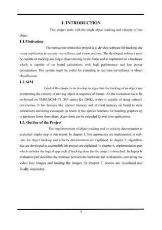
  • 33. 7. RESULTS Object tracking, the main application for security, surveillance and vision analysis, is evaluated on MATLAB/SIMULATION by using the code composer studio, the interface to deploy the algorithms from the workstation to TMS320C6416T. In this, a video is recorded using digital camera. The recorded video frames are converted into individual frame and then converted into Portable Gray Map (PGM) format images. C language code is implemented to convert the pixel values in the PGM format image into Hexadecimal values and store the values in the files, which are inputs for code composer studio. The implementation part starts when the images in Hexadecimal format are imported into code composer studio. In the implementation part, noise is removed for the imported images using median filter. The filtered images are used as input for the frame difference for the separation of foreground and background objects. A rectangular bounding box is plotted around the foreground objects produced from frame difference. By using the dimensions of rectangular bounding box, a centroid is plotted. The position of the centroid is stored in the array and the distance is calculated using Eucliden distance formula. The velocity of the object movement 33
  • 34. from frame to frame is calculated by using the distance and frame rate of the recorded video. The velocity is stored in the array. Velocity of moving object is in 2-dimension (since camera is static). Evaluation is now performed on TMS 320C6414T DSK and the values are visualised in the figured. Figure 7.1 shows the step by step process of people tracking a moving object. From this figure it is clear that the inputs and the output produced at each step. Fig 7.1: Block Diagram Of People Trackng SOURCE CODE FOR VIDEO TRACKING clear data disp('input video'); avi = aviread('samplevideo.avi'); video = {avi.cdata}; 34
  • 35. for a = 1:length(video) imagesc(video{a}); axis image off drawnow; end; disp('output video'); tracking(video); %% traking video program function d = tracking(video) if ischar(video) % Load the video from an avi file. avi = aviread(video); pixels = double(cat(4,avi(1:2:end).cdata))/255; clear avi else % Compile the pixel data into a single array pixels = double(cat(4,video{1:2:end}))/255; clear video end % Convert to RGB to GRAY SCALE image. nFrames = size(pixels,4); for f = 1:nFrames % F = getframe(gcf); % [x,map]=frame2im(F); % imwrite (x,'fln.jpg','jpg'); % end pixel(:,:,f) = (rgb2gray(pixels(:,:,:,f))); end rows=240; cols=320; nrames=f; for l = 2:nrames d(:,:,l)=(abs(pixel(:,:,l)-pixel(:,:,l-1))); 35
  • 36. k=d(:,:,l); % imagesc(k); % drawnow; % himage = imshow('d(:,:,l)'); % hfigure = figure; % impixelregionpanel(hfigure, himage); % datar=imageinfo(imagesc(d(:,:,l))); % disp(datar); bw(:,:,l) = im2bw(k, .2); bw1=bwlabel(bw(:,:,l)); imshow(bw(:,:,l)) hold on % % for h=1:rows % for w=1:cols % if(d(:,:,l)< 0.1) % d(h,w,l)=0; % end % end % % end % % disp(d(:,:,l)); % % size(d(:,:,l)) cou=1; for h=1:rows for w=1:cols if(bw(h,w,l)>0.5) % disp(d(h,w,l)); toplen = h; if (cou == 1) tpln=toplen; end cou=cou+1; break 36
  • 37. end end end disp(toplen); coun=1; for w=1:cols for h=1:rows if(bw(h,w,l)>0.5) leftsi = w; if (coun == 1) lftln=leftsi; coun=coun+1; end break end end end disp(leftsi); disp(lftln); % % drawnow; % % d = abs(pixel(:, :, l), pixel(:, :, l-1)); % % disp(d); % s = regionprops(bw1, 'BoundingBox'); % % centroids = cat(1, s.Centroid); % % ang=s.Orientation; % % plot(centroids(:,1), centroids(:,2), 'r*') % for r = 1 : length(s) % rectangle('Position',s(r).BoundingBox,'EdgeColor','r'); % % plot('position',s(r).BoundingBox,'faceregion','r'); % end % % disp(ang); % % imaqmontage(k); widh=leftsi-lftln; 37
  • 38. heig=toplen-tpln; widt=widh/2; disp(widt); heit=heig/2; with=lftln+widt; heth=tpln+heit; wth(l)=with; hth(l)=heth; disp(heit); disp(widh); disp(heig); rectangle('Position',[lftln tpln widh heig],'EdgeColor','r'); disp(with); disp(heth); plot(with,heth, 'g*'); drawnow; hold off end; % wh=square(abs(wth(2)-wth(nrames))); % ht=square(abs(hth(2)-hth(nrames))); % disp(wth(1 % distan=sqrt(wh+ht); % disp(distan); 38
  • 39. Fig:7.1.1. Input Sample Video Fig: 7.1.2.Output Sample Video Of Object Tracking 39
  • 40. 8. CONCLUSION Tracking of moving object is evaluated on MATLAB/SIMULATION which is a major application in security, surveillance and visionanalysis. The MATLAB/SIMULATION external memory is used to store the imported images on board and the implementation is done. The implementation is performed by removing noise in image and separating foreground and background objects. The object is visualized and its centroid is calculated. The distance it moved between frame to frame is stored and using this velocity is calculated with the frame rate of video. The velocity of moving object in 2-dimension (since the camera is static) is determined. In future, algorithms can be implemented on other hardware devices. These algorithms can also be extended for the used of real-time applications and object classifications. BIBLIOGRAPHY 40
  • 41. [1] Gimp software. http://www.gimp.org/downloads/. [2] Image video machine software. http://www.download.com/Image-Video-Machine/ 3000-2186_4-10359035.html. [3] Ulead video studio software. http://www.ulead.com/vs/. [4] MATLAB/SIMULATION technical reference. Technical Report 508035-0001 Rev. A, November 2004. [5] C. Kamath A. Gyaourova and S.-C. Cheung. Block matching for object tracking. https: // computation. llnl. gov/ casc/ sapphire/ pubs/ UCRL-TR-200271. pdf , October 2003. [6] David S. Bright. Removing shot noise from face image. http://www.nist.gov/ lispix/imlab/noise/shotfc.html, May 25 2004. [7] Berthold K. P. Horn and Brian G. Schunck. Determining optical _ow. ARTIFICIAL INTELLIGENCE, pages 389_407, 1992. [8] Jan F. Jørgensen. Mean filter in world wide web. http://www.imagemet.com/ WebHelp/hid_filters_smoothing_mean.htm. [9] Martin Mangard. Motion detection on embedded smart cameras. Master's thesis, Technische Universität Graz, 2006. [10] AshleyWalker Robert Fisher, Simon Perkins and ErikWolfart. Gaussian smoothing in world wide web. http://homepages.inf.ed.ac.uk/rbf/HIPR2/gsmooth.htm, 2003. [11] Ashley Walker Robert Fisher, Simon Perkins and Erik Wolfart. Mean _lter in world wide web. http://homepages.inf.ed.ac.uk/rbf/HIPR2/mean.htm, 2003. [12] Dr. Mike Spann. Image segmentation in world wide web. http://www.eee. bham.ac.uk/spannm/Teaching%20docs/Computer%20Vision%20Course/Image% 20Segmentation.ppt, Course resources for 2008. [13] Alper Yilmaz, Omar Javed, and Mubarak Shah. Object tracking: A survey. ACM Comput. Surv., 38(4):13, 2006. [14] Y. T. Zhou, V. Venkateswar, and R. Chellappa. Edge detection and linear feature extraction using a 2-d random field model. IEEE Trans. Pattern Anal. Mach. Intell., 11(1):84_95, 1989. 41