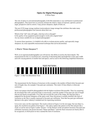
1. Optics for Digital Photography
A White Paper
The role of optics in conventional photography (with film materials) is very well known to professional
photographers. They know how to correctly estimate the relative values of exposure, aperture, picture
angle, perspective and its control, f stop, picture sharpness, depth of field, etc.
The new CCD image storage medium (semiconductor image storage) has attributes that make many
professional photographers feel insecure about their use:
Which of the "old" rules still apply, what has to be re-thought?
Is the quality of my equipment good enough to work with a digital body?
Are my lenses suitable for use in digital photography?
To answer these questions, it is helpful to be able to evaluate picture quality, and especially image
sharpness, by some repeatable measurement technique that can be documented.
1. What is "Picture Sharpness"?
Well, as an experienced photographer you will answer: the ability to resolve the finest details. The
measurement for this is a resolution test, consisting of alternating dark and bright bars of the same width
and with varying patterns of smaller bars and spaces, such as seen in the following simplified illustration.
Figure 1: A Bar Test (Resolution Test)
The measurement for the fineness of structures in this example is the number of black/white line pairs per
unit of length, thus, for example 5 line pairs per centimeter. This totals 10 lines (black or white) per
centimeter.
Such a test pattern should be photographed with the highest resolution film possible. Then, by examining
the developed film with a powerful loupe or microscope, count the number of line pairs per unit of length
that are just barely recognizable. If we take into account the scale of the image, this then provides a
judgment for the picture sharpness of the optics used. Since the picture is usually minified, this limit of
resolution on the film is usually expressed in line pairs per millimeter. Note that line pairs per millimeter
(lp/mm) is the optics' industry's standard unit for expressing resolution
Let us now carry out this experiment. The result is shown in Figure 2 on the next page. Our test object is,
again, the resolution test pattern from Figure 1. The optics capture this pattern on the film and provide a
result, as can be seen in Figure 2 under "picture." As the fineness of the test pattern increases (line pairs per
millimeter increases), the picture becomes "flatter and flatter," until the finest structures are barely able to
be recognized, at which point we have reached the limit of resolution.

2. Figure 2: The Imaging of Structure Details
Brightness distribution: 1 = white paper 0 =black printer
Modulation (MTF) = "Difference in brightness" Modulation as a function of the fineness of lines (No. of
line pairs/mm)

3. If we designate the brightness of pure white paper with a value equal to "1" and the darkness of black
printer's ink with value equal to "0" then the difference in brightness between light and dark bars becomes
smaller and smaller as the number of line pairs increase. This is illustrated in Figure 2 by the diagram
below it:
For the coarse structures, the difference between bright and dark is still equal to 1. For the medium
structures the difference drops to 0.65-0.35 = 0.3, therefore 30%. And for the very fine structures, the
difference is only 5%!
Actually, however, the goal is to capture also the very finest patterns with a great amount bright/
dark difference (high contrast or modulation), so that they remain easily visible!
The limit of resolution alone is therefore not an adequate measurement of picture sharpness; the modulation
with which the pattern is reproduced (in line pairs per millimeter) must also be considered. The higher the
modulation, the better the optics!
We must therefore indicate the modulation of the reproduction as a function of the fineness of the pattern
(in line pairs per millimeter) in a diagram.
This is shown in Figure 2, down at the bottom, where the modulation reproduced for the three line pairs per
millimeter shown in the example is drawn with circles.
The result of our recognition is the modulation transfer function, abbreviated "MTF".
The MTF represents the relationship between the fineness of the pattern (in Lp/mm) and their reproduced
modulation.
Now, a very important question must be clarified: up to what pattern fineness does a modulation transfer
makes sense at all, because what the eye can no longer see does not need to be transferred (imaged).
In this connection, we start from the assumption that the formation of an image does not exceed the printed
format DIN A4 (210 x 297 mm or 8.27 x 11.69 inches) , and that a picture recording format in a somewhat
small size (24 x 36 mm2) is used. This means a magnification of the picture format of about 7-7.5 times.
The usual distance for viewing a DIN A4 document will be about 25 cm ("clear seeing distance"). What
details can the human eye still recognize?
The answer from many practical experiments is: a maximum of 6 line pairs per millimeter (6 Lp/mm)
Converted to the photograph format, this means approximately 7 x 6 = 42 lp/mm, expressed when rounding
the numbers as 40 lp/mm.
In the case of high-quality printing on art printing papers (glossy coated papers), printing is usually done
with a raster width of 150 lines per inch up to a maximum of 200 lines per inch (with 256 shades of gray
and 45° angling).
This is therefore about 6-8 lines/mm and therefore 3-4 line pairs/mm. Consequently, even from this point
of view, the 6 lp/mm is a reasonable upper limit. Anything above that is neither resolved nor recognized by
the human eye. However, the highest possible modulation transfer (MTF) is definitely desirable and may be
perceived with this line pair number!
A very clear representation of these facts was given as early as 1976 by Heynacher and Köber[1], who's
explanation with sample images is highly recommended for reading.
In order to carry the pure indication of a resolution value completely to the limit, a simple calculation
example can be considered:

4. Assume that we use the highest resolution film with excellent optics, which together can reproduce about
75 lp/mm.
Enlarged by a factor of 7.5, this results in the resolution limit in the image of 10 Lp/mm, which the eye can
no longer resolve!
Decisively more important is the degree of the modulation reproduced up to the resolution limit of the eye;
that is 6 Lp/mm in the magnification or 6 x 7.5 = 45 Lp/mm on the film!
This example can also easily be transferred to other film formats. Thus, for the format of 9 x 12 cm (4 x 5
inches), the line pair number limit to be considered is at about 20 lp/mm, even with a substantially larger
final format.
You may now wonder what these tests with simple bar grids and patterns have to do with reality, where
complicated structures having soft tone transitions and fine surface details occur simultaneously, such as on
a sand surface lighted from the side. If we are to be scientifically accurate, the answer is fairly complicated,
but it can be reduced to a simple denominator. Every brightness and pattern distribution in the test subject
can be thought of as being composed of a sum of periodic structures of different fineness and orientation.
The bar tests are only a simple example. Under actual photographic conditions, instead of the abrupt bright-
dark transitions of our test patterns, only softer transitions have to be considered, with a "more harmonic"
progress and more precisely sinusoidal changes.
The sum of all these lines (line pairs/mm) of different orientation comprise the object structure. The object
is then offered to the lens for portrayal in the image plane. The lens weakens the contrast of the individual
components according to its modulation transfer function and produces an image, which corresponds more
or less well to the object.
In this regard, the answer to the question posed at the beginning, "What actually is picture sharpness?"
becomes apparent. Picture sharpness is:
- The highest possible modulation reproduction for coarse and fine object structures (expressed in line
pairs per mm), up to a maximum line pair number dependent on the application.
- This limit depends on the format of the photograph and the intended final enlargement and is
decisively affected by the highest line pair number that the eye can recognize in the final enlargement
(about 6 lp/mm).
Figure 3 summarizes this again graphically:
1. low modulation, high resolution Lp/mm
2. high modulation, less resolution = better quality
3. high modulation, high resolution = no improvement in quality

5. Figure 3: Different MTF Characteristics
2. Digital Photography Part I - Format Constraints
After the above discussions of image sharpness and modulation transfer, you will undoubtedly already
recognize the following principle for the requirements of digital photography, in that it is linked to the
format of the image sensor. The smallest representable image element of a semiconductor image sensor
(Charged Coupled Device or CCD) is called a "pixel," which is an abbreviation for the expression "picture
element." By loose analogy, this could be designated as the grain of digital photography. Unlike film grain,
the pixel has a strictly regular geometric structure and is arranged in rows with a square or rectangular
surface. Today's high-performance image sensors (at affordable prices) have pixel numbers of 2,000 x
2,000 pixels to 2,000 x 3,000 pixels. The size of these pixels are about 0.015 mm to 0.012 mm. This results
in a format of the image sensor of about 30 x 30 mm or 24 x 36 mm - or just about that of the 35mm film
format.
Therefore, we can transfer the results concerning image sharpness as follows:
The lens must transmit up to 40 Lp/mm with the highest possible modulation.
One precondition is important in this regard: The image sensor must transmit this line pair number
with the highest possible modulation as well!
The sensor can transmit these line pair numbers only if a dark bar falls specifically on a pixel and a bright
bar on the neighboring pixel.
Or, conversely:

6. The highest line pair number, which a sensor with a pixel dimension "p" can transmit, is equal to:
RMAX = Lp/mm
In the above examples, this is 33 Lp/mm (for pixel size 0.015 mm) and 40 Lp/mm (for pixel size 0.012
mm).
With the first-named sensor (pixel size .015 mm), you do not entirely achieve (according to our current
state of knowledge) the image quality sought (with a final image of about DIN A4), but with the second
sensor (pixel size .012 mm) you just achieve the image quality sought. It will be seen in the next section
that still further sensor-specific characteristics must be taken into consideration, which are connected with
regular pixel structure. But before that, we need to address a few additional points that are associated with
the changed format.
Further Format Related Considerations:
*Focal Length, Image Angles
In the past, if you have worked with a large-format camera (9 x 12 or 4 x 5 inch) and now wish to use a
digital body with one of the sensors we have discussed, then you must consider that the format, related to
the picture diagonal, has decreased in size by a factor of about 3.5. In order to obtain the customary image
angle, you must therefore use a 3.5-times shorter focal length.
Format 9 x 12 cm 24 x 36 mm
Focal lengths 90 mm 150 mm 210 mm 360 mm 25 mm 43 mm 60 mm 103 mm
Highest number of Lp/mm 20 Lp/mm (better than DIN A4 40 Lp/mm (for about DIN A4
final format) final format)
Table: Focal lengths for approximately the same image angle,
If work is to be done in digital photography with these sensors with perspective correction (shift and tilt) as
well, then the image circle diameter of this lens must of course be larger than the image diagonal (for
example, about 60 mm).
********
*Depth of field and corresponding Tables.
The depth of field depends upon the permissible circle of confusion diameter. This is standardized and, for
the 9 x 12 cm format, is 0.1 mm and for the 35-millimeter format, 0.033 mm. These numbers are based on
the assumption that the final enlargement (or the copy) has a 9 x 12 format. Then this circle of confusion
diameter can hardly be perceived by eye (at an observation distance of 25 cm). However, since we have
assumed a double-size final format, the circle of confusion diameter should be only half as big, in order to
maintain sufficient image quality even at the edge of the depth of field. Naturally, the depth of field is also
reduced by half.
Please note however:
As a result of the smaller format, the image scale is also decreased in order to portray the same object fully
sized on the format. If we refer to the format diagonals (in order to get away from the differing side ratios),
the following picture results:

7. Format Diagonal
9 x 12 cm = 150 mm
24 x 36 mm = 43.2 mm
The ratio of the diagonals is therefore approximately
V = 1 : 3.5
The imaging scale for the 35-millimeter format must also be reduced by this ratio. Using the depth of field
formulas, it can then be shown that the f-stop number can be decreased by the same factor V, with the same
depth of field T. Thus if, in the large picture format, you work with f-stop f/22, then in the case of the 35-
millimeter format you can obtain the same depth of field with the f-stop f/22 ¸ 3.5 = 6.3. This is an aperture
of 5.6 plus 1/3 of an aperture.
The following table should make this clearer on the basis of an example:
Large format f/22 d' = 50 µm 35 mm format f/6.3 d' = 15 µm
ß T/mm ß T/mm
1/10 1/20 1/30 242 924 2046 1/35 1/70 1/105 238 939 2103
KEY TO ABOVE CHART:
ß = Magnification (or image scale)
d' = Circle of Confusion
3. Digital Photography Part II - The Limits of Image Sensors
The tendency in the semiconductor industry to house smaller and smaller structures in the tiniest space has
its driving force in the fact that the cost of a component (for example, an image sensor) increases at least in
proportion to the surface area. Currently, the size of the smallest reproducible structures are 1/4 µm (that is,
1/4 of a thousandth of a millimeter!). In the research laboratories of the semiconductor industry, they are
working on achieving still smaller structures, down to 1/10 µm. It is therefore reasonable to assume that
this development will benefit semiconductor image sensors as well, with a lower limit for the pixel size
being imposed by a decreasing sensitivity. This limit will, however, not be smaller than 5 µm, as in modern
¼-inch format CCDs typically used in C-mount cameras.
Then there exists the possibility (1) of reducing the surface area of the sensor with the same number of
pixels, in order to make it less expensive, or (2) of increasing the number of pixels in the same surface in
order to increase image quality and push it in the direction of the medium format.
This should be explained by the example of the sensor with the 35-millimeter format and a pixel size of
12µm (2K x 3K sensor).
Decreasing the pixel size to 6 µm means:
In case (1): Reduction of the surface to 1/4 (12 x 18 mm)
Number of pixels 2K x 3K = 6 million pixels, as before
In case (2): Same surface (24 x 36 mm) as before, and
An increase of the number of pixels to 4K x 6K = 24 million pixels
In each case, as a result, the highest number of line pairs, which the new sensor can transmit is doubled,

8. Size (Pixel) Resolution
p1 12 µm = 0.012 mm => 40 Lp/mm = R1max
p2 6 µm = 0.006 mm => 80 Lp/mm = R2max
Another special fact about digital image memories must be taken into account; it has to do with the regular
arrangement of pixels as opposed to the irregular grain structure of a film.
If we examine more carefully the modulation transfer of the digital image memory in the vicinity of the
highest transferable pair of lines Rmax (maximum resolution), then we note that for greater numbers the
modulation does not suddenly fall to zero; instead, there is a characteristic decrease in the line pair number
reproduced. The following Figure 4 should clarify this.
Figure 4: The Reproduction of Structure Details over the Limit of Resolution of the Image Sensor

9. The bar test can be seen in the Figure at the top, as well as the associated brightness distribution between 1
and 0 of the bright and dark bars. On the horizontal axis, the dimensions of the pixels are shown, in the
example from pixel No. 1 through pixel No. 40. One recognizes that there are about 7 bright/dark bar pairs
(line pairs) for 10 pixels. The bar widths are now smaller than a pixel (by a factor of approximately 0.7), so
that a bright bar but also a certain portion of a dark bar falls onto a single pixel. The pixel can no longer
distinguish between these and averages the brightness (in approximately the same way as an integrating
exposure meter). Therefore, the succeeding pixels now have differently bright gray tones, depending on the
surface portion of the bright and dark bars on the pixel, as can be seen in the middle of Figure 4. The
brightness distribution below shows that now only three (roughly stepped) transitions from maximum
brightness to maximum darkness per 10 pixels occur. Actually, however, there should be 7 line pairs per 10
pixels, as in the test pattern. The line pair number reproduced therefore decreased instead of
increasing. The image no longer matches the object, it consists only of false information! If we consider
that the highest transferable line pair number is equal to 5 line pairs per 10 pixels, then we also recognize
the mathematical relationship for this characteristic information loss: the line pairs exceeding the maximum
line pair number of 5 Lp/10 pixels (7 Lp/10 pixels - 5 Lp/10 pixels = 2 Lp/10 pixels) are subtracted from
the maximum reproducible line pair number (5 Lp/10 pixels - 2 Lp/10 pixels = 3 Lp/10 pixels) and
therefore result in the actually reproduced (false) structure of 3 Lp/10 pixels. The modulation transfer
function is therefore mirrored at the maximum reproducible line pair number Rmax, as shown in
Figure 4, bottom.
Naturally, we are not interested in the reproduction of this false information and it would be ideal if the
modulation transferred would suddenly drop to zero at the maximum line pair number. Unfortunately, this
is not possible, either for the optics or the image sensor.
We must therefore pay attention that the total modulation transferred (from lens and image sensor) at the
maximum line pair number Rmax = (2 x p)-1 is sufficiently small, so that these disturbing patterns are of
no consequence. Otherwise, it can happen that good optics with high modulation are judged to be worse
than inferior optics with a lower modulation.
The total modulation transfer (from lens and semiconductor sensor) is composed of the product of the two
modulation transfer functions. This is also valid for the modulation at the maximum transferable line pair
number Rmax. For a typical semiconductor image sensor, the modulation at Rmax is about 30-50%.
Therefore it is reasonable to demand about 20% for the optics at this line pair number Rmax, so that the
false information will definitely lie below 10% (0.5 x 0.2 = 0.1).
Our knowledge from the format-bound arrangement must therefore be supplemented:
(1) The modulation transferred at the highest line pair number Rmax, which can be reproduced by the
sensor, must be sufficiently small so that no false information is transferred.
(2) On the other hand, the modulation transferred must be as high as possible at the highest identifiable line
pair number, determined by the format enlargement and the resolution power of the eye.
This contradiction can only be resolved if the limit line pair number of the sensor (Rmax) is significantly
higher than the maximum line pair number resolved by the eye. Let us explain this using the (hypothetical)
image sensor with a 6 µm pixel distance and 4K x 6K = 24 million pixels (format 24 x 36 mm) as example:
In this case the limit line pair number of the sensor (Rmax) is at 80 Lp/mm. At this line pair number the
modulation (from sensor and optics) must be low, as shown earlier in this paper. But the highest
identifiable line pair number for the 24 x 36 mm² format is only about 40 Lp/mm (with magnification 7x
and 6 Lp/mm resolving power of the eye), so that there is still sufficient reserve for the highest possible
MTF at this line pair number.
Independently of these considerations, we must also take into account that color fringes (resulting from
chromatic aberrations) are of course disturbing (as in classical photography). The color fringes should be
significantly smaller than a pixel size, which can only be achieved by using top quality lenses made with
special glass having so-called apochromatic (high color correction) construction.

10. 4. Lenses for Digital Photography - a New Series from Schneider Kreuznach
At Photokina '98, Schneider Kreuznach presented a new series of lenses which optimized for digital
photography. The new name -- DIGITAR -- should lead the way in digital photography.
The focal lengths range from 28 to 150 mm with image circle diameters of 60 mm and above, and are
therefore most suitable for high resolution digital photography with current image sensors. As a result of
their MTF values and the apochromatic correction, they are also largely suitable for image sensors of the
next generation.