Many sites along the Apulian coast (SE Italy) are composed of weathered and fractured carbonate rocks, affected by intense erosion and frequent sliding. A detailed research of the University of Bari (Andriani and Walsh, 2007) highlighted that from 1997 through 2003, the cliff retreat rate varied from 0.01 to 0.1 myr-1, mostly as a consequence of wave action. In the case of Polignano a Mare, a small town 30 km far from Bari, the erosive process seems to be seriously affecting the stability of buildings. Here, because of the bathymetry, the traditional rubble mound breakwaters are not suited. As an alternative, a rigid horizontal submerged plate on piles is here considered. Since there is no universally accepted theory nor formula to calculate the hydraulic performance of such kind of structure physical models have been constructed at HR Wallingford and subjected to random wave attacks. This paper discusses results of those tests.

1. SUBMERGED HORIZONTAL PLATE FOR COASTAL RETREATING
CONTROL: THE CASE OF POLIGNANO A MARE, ITALY.
M. Calabrese1, K. Powell2, M. Marrone3,
M. Buccino1
Many sites along the Apulian coast (SE Italy) are composed of weathered and fractured carbonate
rocks, affected by intense erosion and frequent sliding. A detailed research of the University of Bari
(Andriani and Walsh, 2007) highlighted that from 1997 through 2003, the cliff retreat rate varied
from 0.01 to 0.1 myr-1, mostly as a consequence of wave action. In the case of Polignano a Mare, a
small town 30 km far from Bari, the erosive process seems to be seriously affecting the stability of
buildings. Here, because of the bathymetry, the traditional rubble mound breakwaters are not suited.
As an alternative, a rigid horizontal submerged plate on piles is here considered. Since there is no
universally accepted theory nor formula to calculate the hydraulic performance of such kind of
structure physical models have been constructed at HR Wallingford and subjected to random wave
attacks. This paper discusses results of those tests.
INTRODUCTION
The main scope of a structural measure for coastal erosion control is indeed
reducing the intensity of wave attacks in the nearshore. Yet, in most of cases
also a small intrusion in the landscape is requested. For this reason underwater
barriers are now becoming rather popular, especially in sites, like the Italian
coasts, where tidal range is small. Submerged barriers are traditionally
multilayered rubble mound breakwaters that force the waves to break and reduce
their power. Generally they are located on a limited depth and may be both
narrow and wide crested, depending on the degree of wave energy which is
considered to fit a given design situation.
Clearly, as soon as the depth of placement increases, the use of traditional
breakwaters becomes anti-economical and non conventional solutions have to be
considered.
This may be the case of Polignano a Mare, a small town 30 km far from Bari
(Italy), where the erosion process is of such a severity to affect the safety of
buildings. As many sites along the Apulian coasts, Polignano a Mare is located
on weathered and fractured carbonate rocks that experienced intense erosion
and frequent sliding. Here the sea bottom is 25m depth at a few meters from the
coastline and accordingly the construction of traditional barriers is strongly
discouraged.
As an alternative, a rigid horizontal plate on piles is being considered by HR
Wallingford. Since no well accepted theory nor empirical formula exists to
predict the hydraulic response of such a structure (Patarapanich and Cheong,
1989; Yu et al., 2002), ad hoc random wave tests have been conducted.
1Hydraulic department, University of Naples “Federico II, Via Claudio, Naples, Italy. Email: calabres@unina.it,
buccino@unina.it
2HR Wallingford, Howbery park, OX , Wallingford, Email: k.powell@hrwallingford.co.uk
3Engineer, Email: marcomarrone83@hotmail.it

2. This paper analyses results of those experiments, with the aim of providing
engineers with two simple predictive methods: one permits of estimating the rate
of energy that is reflected back by the structure and the other allows of
calculating the wave height transmitted off the barrier.
FACILITIES AND DATA DESCRIPTION
The models have been tested in the random wave flume of the HR Wallingford’s
Flume Hall. The flume was 45 m long, 1 m wide and 1.5 m high.
Waves were first calibrated in the model, before the placement of the structure,
with the aim of reproducing the same wave conditions as those recorded in
Polignano a Mare. With this purpose, a (short) signal sample was first adjusted
to ensure the spectral significant wave height, Hm0, was within +/-5% of the
target value. Then, a long (1000 waves) non-repeating wave sequence was run to
simulate the actual incident sea-state; main wave parameters are reported in
Table 1.
Table 1 – Results of wave calibration
Period H1/10 H1/3 Hm0 Tp Tm
of
return (m) (m) (m) (s) (s)
1 in 1 4.91 3.95 4.06 8.98 7.44
1 in 10 6.25 5.02 5.18 9.95 8.52
1 in 50 7.20 5.81 6.00 11.60 8.78
After the calibration, the plate was built in the flume at a distance of 10m from
the wave paddle. The width of the structure, B (Figure 1), ranged from 25 and
55m (prototype scale); two depths of submergence, d’, have been tested, namely
2,5 and 5m. Altogether, 42 tests were run.
H'
HI HT
L L' LT
d'
B
d
Fig. 1 – Structure scheme

3. GLOBAL FEATURES OF THE WAVE MOTION
The coefficient of reflection
The reflection coefficient, Kr, square root of the reflected to incident spectral
areas, has been estimated through the Mansard and Funke’s separation
technique (1980), which requires the simultaneous acquisition of the wave
elevation process at three different positions along the propagation’s direction.
From a physical point of view, wave reflection is likely related to the presence
of a pulsating flow driven by the phase shift between the incident and the
transmitted wave. Following Graw (1992), we may reason the momentum flux
of this current to act more or less like a wall that impedes the propagation of the
pressure wave below the plate. Thus, a coherent functional form of the
coefficient of reflection might be:
 2B 
K r  A  sen  (2)
 RL 
in which A represents the maximum of Kr, which is attained at the point of phase
opposition, and R defines the structural condition where such a critical situation
occurs; in this regard previous literature seems to indicate R should not be far
from 2, so that the maximum reflection would correspond to kB=π. Here the
following empirical expressions have been obtained:
 H 
A  tanh 204 si2  (3)
 gT p 
 
0 , 57
 d 
R  9,5 2  (4)
 gT 
 p 
Note that Equation (4) gives values of R around 2 only for relatively deep water
(d/L0p, from 0.2 to 0.4, being L0p the peak deepwater wavelength), while the
maximum reflection would be attained for shorter structures as the depth of
placement becomes shallow. Fig. 2 shows the comparison with the experimental
data. Together with the line of perfect agreement, two semi bands corresponding
to an error of 15% are reported in the graph.

4. 0,9
Dati
Kr, estim.. Perfect match
-15%
+15%
0,6
0,3
0
0 0,3 0,6 Kr, meas. 0,9
Fig. 2 – Comparison between the formula 2 and the experimental data
However, as shown in the previous figure, present data oscillate in a quite
narrow range around the value 0.7; consequently, some further indication on the
reliability of the proposed equation has to be achieved using other available
data. For this purpose experiments by Yu et al. (1995) have been employed,
although they have been performed using regular waves. The tests refer to a
structure placed on a depth of 20cm, with a submergence of 6cm. Wave height
and period were kept constant (H = 1.8cm, T = 0.8s), while only the plate width
was varied. The comparison is displayed in Figure 3. The graph shows a fair
match only in the first cycle of variation of Kr, where the main peak appears to
be correctly estimated. On the other hand data exhibit a progressive damping not
predicted in the model. More experiments are recommended to further
investigate this item.
0,6
Kr Eq. 2 Yu et al. Data
0,4
0,2
0
0 0,4 0,8 1,2 1,6
B/L
Fig. 3 – Comparison between the Eq. 2 and the data by Yu et al. (1990) (regular
waves)

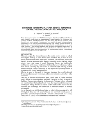
5. Calculation of the significant transmitted wave height
A predictive model for the transmitted, spectrally defined, wave heights, Hm0,t or
Hrms,t is of course important to engineering aims, since these waves are
proportional, at least for linear waves, to the time averaged wave energy leeward
the structure. Obviously, the latter rules most of the shadow-zone
hydrodynamics, including solid transport process, wave run-up as well as the
wave power transferred to any structures lying in the protected area.
It is well known the spectral wave heights can be generally defined as follows:
H m0
H m0  4 m0 ; H rms  8  m0  (5)
2
being m0 the area of the power spectrum.
The calculation method proposed below might be defined as semi-empirical or
“conceptual”; it starts from a quite schematic modeling of main phenomena that
govern wave transmission process and includes a unique free parameter to be
estimated from experimental data. This parameter basically represents the lag of
phase, say ε, between the waves that enter the protected area from above the
plate and those passing below. Breaking process is modeled according to Dally,
Dean and Dalrymple (1985); moreover, an equivalence between regular and the
irregular wave trains is established, by simply substituting the “wave period
averaging operator” by an averaging “in the ensemble domain ”, that is among
the different waves which belong to the sea state (Thornton and Guza, 1983).
Accordingly, under the hypothesis that the power spectrum is narrow enough to
neglect the differences among the single wave periods, we have, for the incident
energy flux:
Pi  g  H 2 f H dH  cg  f p , d   gH rmscg  f p , d 
1  1 2
(6)
8 0 8
in which f(H) is the probability density function (pdf) of the incident wave
height, Hrms is the root mean square wave height and cg(fp,d) is the linear (peak)
group celerity, calculated at the depth of placement d. At the structure, the
incident wave power splits into two parts, one propagating below the plate, Piu,
and another that overpasses the structure, Pio (Fig. 4).
z
x
d'
Pio
Relection Transmission
region region
B
d
Pi Pt
Piu
Pr
Fig. 4 – Scheme of the redistribution of the incident power Pi

6. Regarding the former, we assume it to equal the time averaged energy flux, per
unit of span, through a section of height (d – d’). Consistently with the general
approach above discussed, we first calculate that quantity for a single wave and
then we average the result on the wave ensemble. Consequently we obtain:

Piu   Piu f H dH
H
(7)
0
in which PiuH is the under-passing power for a single wave that is given by:
1 T d '
Piu  0 dt d pi ui dz
H H H
(8)
T
where pi represents the (incident) dynamic component of pressure, ui is the
horizontal component of wave velocity and the prime H has been introduced just
to highlight that the calculated quantity refers to the single wave. Using linear
wave theory one readily gets:
1 1  d  d '2k  senh2k d  d '
Piu  gH i2c 
H
 (9)
8 2 senh2kd  
in which c is the incident phase speed and k represents the wave number, k=2π/L
(L is the incident wavelength). Finally, by invoking the hypothesis of narrow
banded spectrum, we have:
Piu 
1
gH rmsi c 
 
1  d  d '2k p  senh 2k p d  d ' 

2
senh2k p d 
(10)
8 2 

in which the subscript p indicates a “peak quantity” and i stands for “incident”.
Note that as a consequence of having adopted the linear wave theory in the
calculations, equation (10) gives no flux below the plate when d’=0. This
hypothesis limits the application of the model to the case of a plate not very
close to the mean sea level. The power Piu is supposed to undergo no remarkable
dissipation, but it will not entirely propagate to the protected area, due to
reflection effects. Accordingly the energy flux transmitted below the structure
will be equal to:
Ptu  Piu  K r2 Pi (11)
It is worth underlining that the coefficient of reflection, Kr, calculated by the
formulas (2) – (4), is already a global quantity referred to the ensemble and then
it does not need require any statistical manipulation.
Now it is clear that the part of the incident power that overtops the structure
equals:
Pio  Pi  Piu (12)
Obviously this portion of flux is remarkably diminished by wave breaking. As
already mentioned, here we suppose, in agreement with Dally, Dean and
Dalrymple (1985), the average power density dissipated by a single breaker to
be proportional to the difference between the local wave energy flux, say PHo,
and a stable value, say Ps; moreover dissipation is thought to be inversely

7. proportional to the available depth, d’ (Fig. 4). This leads to the following
expression:
D  l
Po
H
 Ps  (13)
d'
in which l is a coefficient of proportionality that Dally, Dean and Dalrymple
fixed to the value 0,15. Altogether the energy balance equation above the plate,
for the single wave, can be t written as follows:
dPoH
 l o

P H  Ps  (14)
dx d'
Since Ps does not vary along x, as the plate is horizontal, variables can be
separated. Hence we have:

d PoH  Ps 
 l
dx

Po  Ps
H
 d'
(15)
Integrating between 0 and B with the initial condition that PoH– Ps=PHio – Ps for
x=0 (the suffix “i" indicates the incident value of the flux above the plate), we
obtain:
 
 B
Pto B   Ps  Pio  Ps exp   0.15 
H H
(16)
 d' 
Moving from the single wave to the whole sea state, we will notice that the
energy flux in the plate’s terminal section will be equal to the Equation (19) only
for those waves breaking on the structure; on the other hand the transmitted flux
will be equal to PioH for the waves that will not break. The mean value of the
power transmitted above the structure will be then equal to:
 
Pto   Pto B  f b H dH  Pio  f nb H dH
H H
(17)
0 0
in which fb and fnb are the pdf of the breaking and non breaking waves
respectively. In agreement with Thornton and Guza (1983), the easiest way to
estimate such functions is to consider them proportional to the general wave
height pdf, f(H):
 f b H dH  Pb f H dH

 f nb H dH  1  Pb  f H dH
(18)
where Pb is the percentage of breaking waves. Finally we have:
Pto  Pb  Ptob  1  Pb Ptonb (19)
in which Ptob represents the transmitted energy flux for breaking waves:

 B
Ptob   Pto B  f H dH  Ps  Pio  Ps  exp   0,15 
H
(20)
0  d' 
while for the energy flux connected to the non-breaking waves, Ptonb, we will
simply set:

8. Ptonb  Pio (21)
In the previous integration we considered the stable flux, Ps, as independent of
the wave height. Basically we set:
1
Ps  gH b2 C gpd' (22)
8
where Cgpd’ represents the linear peak group speed corresponding to the depth of
submergence d’. As far as the incipient breaking wave height, Hb, is concerned,
the well known Mc Cowen criterion has been employed:
H b  0,78d ' (23)
As regards to the percentage of breaking waves, Pb, it has been assumed it to be
simply equal to the exceedance probability of, Hb, under the hypothesis that
overpassing waves at the seaward edge of the plate are Rayleigh-distributed:
 H2 
Pb  exp   b 
 8m  (24)
 0o 
in which m0o is the specific energy of the wave motion above the plate at the
leading edge of the structure; it is equal to:
Pio
m0 o  (25)
gc gp,d '
Now, the wave field at the back of the structure will be composed of two
different subsets of waves, respectively coming from above and below the plate.
They propagate in the same direction but with different phases owing to the lag
of celerity above and below the scaffolding. Thus we may describe the single
wave elevation process as follows:
cos  p t   tu cos p t   
H to H
 t H  t   (26)
2 2
in which Htu and Hto represent respectively the underpassing and overpassing
transmitted wave heights, while the symbol ε indicates their difference of phase.
Finally to calculate the transmitted wave energy m0t, we introduce the
fundamental relation, valid for linear sea states:
m0  VAR     2 (27)
in which VAR indicates the variance operator and the “overbar” symbol
indicates a time average. Following the simplified approach previously
proposed, the calculation of m0 will be performed in two steps, namely:
1. Firstly we calculate the η variance referred to the single wave by an average
over a wave period:
T
1 2 H 
 t2 H  
T
 t dt (28)
o

9. 2. then we estimate the overall sea state energy by averaging t2H  over the
ensemble of waves, that is among the different wave heights:
m0t  t2  E t   
2 H
(29)

 

It can be easily shown that aforementioned steps lead to:
 
m0 t  E  2  H  
8
H rms,to  H rms,tu  2H rms,to H rms,tu cos  
1 2 2
(30)
that holds under the hypothesis that the skewness of the transmitted wave pdf is
rather small. Hrms,to and Hrms,tu can be simply obtained as
Pto
H rms,to  8m0,to  8 (31)
C gpd
Ptu
H rms,tu  8m0,tu  8 (32)
C gpd
In the Equation (30) ε has been treated as a free parameter and its value has been
optimized experiment by experiment. Then a multiple regression analysis has
been performed in order to relate the optimized values to the main structural and
hydraulic parameters. The following final equation has been found:
  1,77 exp  0,7011  k p d ' k p B 
' ' 0, 291
(33)
where k’p represents the peak frequency wave number calculated at the
submergence level d’. Note that Equation (33) realistically returns a null phase
shift either for extremely short or deeply submerged structures.
The Fig.(8) shows the comparison with the experimental data in terms of
Hrms=8m0t. The agreement can be considered reasonable. The maximum
difference between the measured and the calculated values are of about 20% and
the global determination index is 81%.

10. 5
Ht, meas. Data
Perfect match
-20%
4 +20%
3
2
1
0
0 1 2 3 4 5
Ht, estim.
Fig. 8 – Comparison among the measured and the estimated values of the wave
heights
SUMMARY
The paper has presented results of hydraulic model tests conducted at HR
Wallingford on a rigid submerged plate on piles. The structure has been
originally thought as a measure for defending the rocky coast of Polignano a
Mare (Italy) from a structural erosive process. The experiments were run using
random sea states representative of the Apulian climate.
The data have been used to derive a predictive method for calculating two
leading hydraulic variables, namely the reflection coefficient and the transmitted
“energetic” (rms, roughly speaking) wave height. The latter is of course of
interesting for every engineer as it is strongly related to the entire shadow-zone
hydrodynamics. As a conclusion of the work a step by step scheme is here
proposed for application scopes.
As far as the reflection coefficient Kr is concerned, Eq. (2)-(4) have to be used.
However caution is recommended when applying the formulas to plates wider
than half the incident peak wavelength.
Regarding the transmitted wave energy the calculation procedure can be
summarized as follows.
a) calculate the phase shift  through Eq.(33); b) calculate Ptu by means of (6),
(10) and (11); c) calculate Pio through Eq.(12) and then Pb by (24) and (25); d)
calculate Ptob and Ptonb by (20),(21) and (22); e) calculate Pto through Eq.(19); f)
calculate Hrms,tu and Hrms,to by means of (31) and (32). Finally the transmitted
wave energy m0t can be obtained through Eq. (30).
REFERENCES:
Andriani G., Walsh N. (2007), “Rocky coast geomorphology and erosional processes: a case study
along the Murgia coastline south of Bari, Apulia – SE Italy” Geomorphology Vol 87, 224 – 238.

11. Graw, K. (1992) “The submerged plate as a wave filter”, Coastal Eng. J., pp.1153-1160.
Mansard, E.P.D. e Funke, E.R., (1980), “The measurement of incident and reflected spectra using
a least square method”, Proc. 17th ICCE, Sydney, pp. 154 – 172
Marrone M. (2008), Master Thesys: “Indagine sperimentale sulla trasmissione a tergo di una
piastra sommersa” Federico II Naples University, Hydraulic geotechnical and environmental
engineering department (in Italian)
Patarapanich M., Cheong H. (1989), “Reflection and transmission characteristics of regular and
random waves from a submerged horizontal plate”, Coastal Eng., Vol. 13, 161 – 182.
Yu X., (2002), “Functional Performance of a submerged and essentially horizontal plate for
offshore wave control: a review”, Coastal Eng. J., Vol. 44, No. 2, 127 – 144.
Yu, X., Isobe, M. and Watanabe, A. (1995), Wave breaking over submerged horizontal plate, J.
Waterway Port Coastal Ocean Eng., 121, 2, March/April, pp. 105-113