We report successful synthesis of low band gap inorganic polyphosphide and TiO2 heterostructures with the aid of short-way transport reactions. Binary and ternary polyphosphides (NaP7, SnIP, and (CuI)3P12) were successfully reacted and deposited into electrochemically fabricated TiO2 nanotubes. Employing vapor phase reaction deposition, the cavities of 100 μm long TiO2 nanotubes were infiltrated; approximately 50% of the nanotube arrays were estimated to be infiltrated in the case of NaP7. Intensive characterization of the hybrid materials with techniques including SEM, FIB, HR-TEM, Raman spectroscopy, XRD, and XPS proved the successful vapor phase deposition and synthesis of the substances on and inside the nanotubes. The polyphosphide@TiO2 hybrids exhibited superior water splitting performance compared to pristine materials and were found to be more active at higher wavelengths. SnIP@TiO2 emerged to be the most active among the polyphosphide@TiO2 materials. The improved photocatalytic performance might be due to Fermi level re-alignment and a lower charge transfer resistance which facilitated better charge separation from inorganic phosphides to TiO2.

1. Supporting Information
Vapor growth of binary and ternary phosphorus-based semiconductors
into TiO2 nanotube arrays and application in visible light driven water
splitting
Ebru Üzer,a Pawan Kumar,b† Ryan Kisslinger,b† Piyush Kar,b Ujwal Kumar Thakur,b Karthik Shankar, b,* and Tom
Nilgesa,*
a.Department of Chemistry, Technical University of Munich, Lichtenbergstr. 4, 85748 Garching b. München, Germany; E-mail: tom.nilges@lrz.tum.de
b.Department of Electrical and Computer Engineering, 9211-116 Street NW, Edmonton, Alberta, Canada T6G 1H9; E-mail: kshankar@ualberta.ca
†Contributed equally
1. Experimental details
Fabrication of TiO2 nanotube membranes
TiO2 nanotube membranes were fabricated through anodization.1 Titanium foil was used as both the anode and
cathode; the anode was 4 cm long and 1 cm wide, while the cathode was 2 cm long and 0.5 cm wide. Both the
cathode and anode were 0.89 mm thick. The electrolyte was comprised of 97:3 v/v ethylene glycol and deionized
water, with 0.03 wt.% NH4F added in. The electrolyte was stirred vigorously before anodization. The anode and
cathode were spaced 2 cm in the solution, and the 100 mL beaker containing the electrolyte submerged in a water
bath for cooling. A voltage of 60 V was applied for 3 d to create the nanotube arrays; they were then dipped in
methanol for cleaning, and the 0.89 mm thick sides of the anodized pieces scratched off with a razor to allow them
to delaminate during subsequent air drying. To open the bottoms of the nanotubes and clean the tops of any debris,
the delaminated nanotube arrays (membranes) were subjected to reactive ion etching using Oxford PlasmaPro
NGP80. An SF6 etch using a pressure of 20 mTorr and a forward power of 250 W was used for 200 s on the top and
300 s on the bottom (see Results and Discussion for explanation of our top versus bottom terminology). An oxygen
cleaning using a pressure of 150 mTorr and a forward power of 225 W for 10 min was used on each side.
Synthesis of hybrid NaPx@TiO2 nanotube membranes
The chemical vapour deposition of NaP7 and NaP15 on TiO2 nanotube membranes was synthesized according to
literature procedures.2 A mixture of the elements sodium and red phosphorus in the atomic ratio of 1:7 was
prepared by transferring red Phosphorus (452.1 mg, 99.999+%, Chempur) and Sodium (47.9 mg, 99,95% in oil,
Aldrich) into a silica-glass tube (0.8 cm inner diameter, 8 cm length). Into the previously graphitized glass tube,
purified CuI (10 mg) together with TiO2 nanotube membranes was added. The ampoule was sealed under vacuum
(p < 10−3 mbar) and placed horizontally in the chamber of a muffle furnace to obtain a temperature gradient of
approx. 10 K. By locating the starting materials in the hot zone of a Nabertherm muffle furnace (L3/11/330) and TiO2
nanotube membranes in the colder zone, a dissolution via gas phase and deposition on the TiO2 nanotube
membranes was attempted. The furnace was set to 823 K within 10 h and held at this temperature for 7 d. The
products were formed after cooling down by switching off the furnace. Deposition of thin red-brown fibres on the
TiO2 nanotube arrays were observed. Red, block-like crystals of NaP7 were formed simultaneously.
Purification of the mineralizer CuI was carried out by solving CuI (98+%, Chempur) in concentrated HI (57 %, Riedel
de Häen) and following precipitation in water. The precipitate was purified by washing twice with water and ethanol
and subsequently dried under vacuum.
Synthesis of hybrid SnIP@TiO2 nanotube membranes
The preparation of hybrid SnIP@TiO2 nanotube membranes was carried out following the bulk-SnIP literature
procedure.3 The starting materials Sn (107.8 mg, 99,999%, Chempur), SnI4 (189.6 mg, synthesized according to
literature procedures),4 and red phosphorus (37.5 mg, 99.999+%, Chempur) were pressed into a pellet (diameter:
10 mm, 25 MPa for 15 min). The pellet and TiO2 nanotube membranes were transferred into a silica glass tube, the
ampoule was sealed under vacuum (p < 10−3 mbar) and placed horizontally in a Nabertherm muffle furnace
(L3/11/330). The materials were located at the hot zone at 923 K and the membranes at the colder zone of the
furnace. Cooling the melt down to 773 K within 15 h at a rate of 2 K h-1 and of 1 K h-1 to room temperature led to
deposition of SnIP onto the TiO2 nanotube membranes.
Electronic Supplementary Material (ESI) for Nanoscale Advances.
This journal is © The Royal Society of Chemistry 2019

2. Synthesis of (CuI)3P12@TiO2 nanotube membranes
The synthesis of (CuI)3P12@TiO2 nanotube membranes was attained according to literature procedures.5 Purified CuI
(181.8 mg) and red Phosphorus (118.2 mg, 99.999+%, Chempur) were pressed into a pellet (diameter 10 mm,
25 MPa for 15 min). The pellet was placed in a silica glass tube (0.8 cm inner diameter, 8 cm length) with TiO2
nanotube membranes, located at the opposite side. The ampoule was sealed under vacuum (p < 10−3 mbar) and laid
horizontally in a Nabertherm muffle furnace (L3/11/330) so that the starting materials are located at the hot zone
of the furnace and the TiO2 nanotube membranes at the colder zone. The furnace was heated to 773 K within 8 h,
with a holding period of 48 h, cooled down to 673 K within 24 h and held at this temperature for 11 d. Room
temperature was reached within 24 h.
CuI was purified as it was mentioned in a previous paragraph.
Synthesis of polyphosphide@TiO2 nanotube hybrids
TiO2 nanotube membranes were prepared by electrochemical anodization of titanium foil to produce an ordered
array of parallel-aligned TiO2 nanotubes. The membranes had two distinct sides: a side that was exposed to the
electrolyte during the anodization process (top side) and a side that was delaminated from the underlying titanium
substrate (bottom side). Owing to the fluoride etching process during anodization, the top side had thinner sidewalls
and thus large inner tube diameter. The nanotube bottoms had an average inner diameter of 67±9 nm (n = 50
nanotubes), shown in Figure 1b; the nanotube tops had an average inner diameter of 120±13 nm (n = 50 nanotubes),
shown in Figure 1c. To maximize the probability of deposition inside of the tubes, the nanotubes were placed top
side up in the ampoule. To fabricate hybrid semiconducting materials, we succeeded in filling the anatase-type TiO2
nanotubes with binary NaP7/NaP15, and ternary (CuI)3P12, SnIP using a short-way transport reaction; this reaction is
adapted from the so-called mineralization-principle used for the synthesis of a plethora of phosphorus-containing
compounds. Notably, owing to the TiO2 nanotube structure necessary to deposit sodium polyphosphides on and
inside the membranes, the structure withstood the thermal treatment and led to deposition of respective
polyphosphides onto and into the membranes.
1.1 Physicochemical characterization
X-ray powder diffraction
X-ray powder data were collected on a Stoe STADI P diffractometer (Cu-Kα1 radiation, λ = 1.54060 Å, Ge-
monochromator) fitted with a Mythen 1 K detector (Fa. Dectris). An external calibration was performed using a
silicon standard (a = 5.43088 Å). Phase analysis and indexing was carried out with the program package Stoe
WinXPOW.6
Scanning Electron Microscopy (SEM) and Energy Dispersive X-ray spectroscopy (EDS).
TiO2 nanotubes and according nanofibers were investigated via Scanning Electron Microscopy with a SEM JCM-6000
NeoScop TM (JEOL, 5900LV, Si(Li) detector). The compositions of the hybrid compounds were determined semi-
quantitatively by EDS measurements (Energy Dispersive X-ray Spectroscopy, Röntec). The samples were applied with
an acceleration voltage of 15 kV. The measured composition is in good agreement with the composition achieved
from structure refinement.
Scanning Transmission Electron Microscope (STEM) and Energy Dispersive X-ray spectroscopy (EDS).
STEM-EDS analysis was performed on a JEOL JEM-ARM200cF STEM, which is equipped with a cold Field-Emission
Gun (cFEG) and a probe Cs corrector. EDS maps were acquired with a Silicon Drift (SDD) EDS detector at an
acceleration voltage of 200 kV.
Helium Ion Microscope (with Ga-FIB)
For SEM and Auger analysis, samples were prepared using a Zeiss ORION NanoFab Helium Ion Microscope, equipped
with a Ga-FIB column. The cross section of TiO2 nanotubes was milled and polished with a 30 keV Ga-FIB at beam
currents of 1.5 nA.
Raman spectroscopy
Raman studies were performed at 300 K by using a Renishaw inVia RE04 Raman Microscope fitted with a Nd:YAG
laser ( = 532 nm) and a CCD detector. A laser power of 250 mW was applied recording a total number of 500 scans.

3. Auger electron spectroscopy
SEM and Auger measurements were performed using a JAMP-9500F Auger microprobe (JEOL) at the Alberta Centre
for Surface Engineering and Science, University of Alberta. A Schottky Field emitter was used to generate an electron
probe diameter of about 3 to 8 nm at the sample. Sample cleaning was conducted using argon ion sputtering, over
an area of 500 µm2 with a sputtering rate of 15 nm/min as calibrated using SiO2. The SEM and Auger imaging were
performed at an accelerating voltage of 2 kV and emission current of 20 mA. The working distance used was 24 mm.
The sample was rotated 30 degrees away from the primary electron beam to face the electron energy analyzer. For
the Auger spectroscopy and imaging a M5 lens with 0.6 % energy resolution was applied.
X-ray Photoelectron spectroscopy (XPS) and ultraviolet photoelectron spectroscopy (UPS)
The surface chemical composition and oxidation state of materials was determined with X-ray photoelectron
spectroscopy (XPS) by using Axis-Ultra, Kratos Analytical instrument equipped with monochromatic Al-Kα source
(15 kV, 50 W) and photon energy of 1486.7 eV under ultra-high vacuum (UHV ∼10−8 Torr). The binding energy of
C1s of adventitious hydrocarbon (BE ≈ 284.8 eV) was used as standard to assign binding energy (BE) of other
elements by carbon correction. The obtained raw data was deconvoluted in various peak components using CasaXPS
and acquired .csv file were plotted using origin 8.5. To determine the band structure of materials the work function
spectra and valence band spectra of materials were determined by using ultraviolet photoemission spectroscopy
(UPS) with Axis-Ultra, Kratos Analytical instrument and He I line (21.21 eV) of He discharge lamp source.
Additionally, valence band position of bare TiO2 nanotubes was determined with XPS valence band spectra acquired
on Axis-Ultra, Kratos Analytical instrument under ultrahigh vacuum conditions.
Diffuse reflectance UV-Vis (DR-UV-Vis)
Diffuse reflectance UV-Vis spectra to determine UV-Vis absorption profile of materials was acquired on a Perkin
Elmer Lambda-1050 UV–Vis-NIR spectrophotometer equipped with an integrating sphere accessory.
Kelvin Probe Force Microscopy (KPFM)
To discern the charge separation dynamics and validate formation of heterojunction between polyphosphides and
TiO2, the surface potential (SP) or contact potential difference (CPD) of materials was measured using peak force
KPFM (Kelvin probe force microscopy) using Dimension Fast Scan Atomic Force microscope (Bruker Nanoscience
Division, Santa Barbara, CA, USA). For measurements, the materials were deposited on FTO, and a Pt-coated
SiNSCM-PIT cantilever of 2.5 4.4 N/m stiffness was employed to perform the KPFM experiments. Samples were
grounded with the AFM chuck with the help of conductive copper tape. The measurement was performed at zero
tip bias and Pt tip was calibrated by measuring the CPD of HOPG and the Pt tip using following expression:
EF (tip) = 4.6 eV (Work function of HOPG) + VCPD (HOPG and Pt tip)
1.2 Electrochemical characterization
Analytical grade KOH (99.0%), anhydrous Na2SO4 (99.0%), titanium (IV)-isopropoxide (99.99%), were procured from
Sigma Aldrich and used without any further purification. Conductive Fluorine doped tin oxide (FTO) glass
(transmittance 80-82%) was purchased from Hartford Tec Glass Company. The surface of FTO was cleaned by
ultrasonication in water, methanol and acetone for 10 min to remove any residual organics. All the solvent/water
used in the measurements were of HPLC grade.
Photo-electrochemical measurements
The electrochemical properties of the materials were determined by using a CHI660E series electrochemical
workstation in a three-electrode configuration. The photoactive materials deposited on FTO glass containing a TiO2
blocking layer was assigned as anode (working electrode), while Pt sputtered glass and Ag/AgCl was used as cathode
(counter electrode) and as reference electrode respectively. To ensure an equal amount of photocatalytic materials
on the photoanodes, an identical amount of materials, dispersed in methanolic solution was drop-casted on the
exact same area of TiO2 seed layer containing FTO glass. The photoelectrochemical measurements were performed
in 0.1 M KOH aqueous electrolyte. Linear sweep voltammetry (LSV) to measure the materials photocurrent density
was performed by sweeping voltage from –1.0 V to +0.8 V vs Ag/AgCl at a scan rate of 10 mV/sec. The photoanode
was irradiated with solar simulated light (AM1.5 G) having a power density of 100 mW m–2 at the sample surface by
using Newport, Oriel instrument USA, model 67005, solar simulator. To determine visible light response at higher
wavelengths and incident photon-to-current efficiency (IPCE) the samples were irradiated with monochromatic 450
and 505 nm wavelength LEDs having 54.15 and 40.48 mW cm–2 incident power density at the sample surface. Mott-
Schottky plots to calculate flat band potential were extracted from impedance-potential values measure in 0.5 M
Na2SO4 solution in a potential range of –1.0 to +1.0 V at 1 K frequency. Electrochemical impedance spectroscopy
(EIS) to draw Nyquist plots and equivalent circuit under dark and 1 Sun irradiation was performed using a three

4. electrodes configuration at a bias of –0.5 V vs Ag/AgCl in 0.1 M KOH, with an AC amplitude of 0.005 V at frequency
value 1 Hz - 100 kHz.
To investigate the photo-electrochemical performance an approx. 20 nm thick TiO2 blocking layer was spin casted
on cleaned FTO glass using titanium isopropoxide solution according to our previous report just by changing the
dilution of the solution three times.6 The deposition of photoactive materials on TiO2 coated FTO was done by
dispersing materials in very dilute aqueous solution of titanium isopropoxide and drop casting followed by heating
at approx. 150 ºC for 1 h. In this way the materials stick strongly on the TiO2 coated FTO substrate. The materials
deposited on FTO glass function as photoanode (working electrode) and Pt and Ag/AgCl was used as counter
(cathode) and reference electrodes, respectively. The photo-electrochemical water splitting experiments were
performed by immersing the electrodes in 0.1 M KOH solution. The samples were irradiated under solar simulated
light (AM1.5 G) having a power density of 100 mW cm–2 at the sample surface and photocurrent density was
measured in function of applied voltage by sweeping bias from –1.0 V to +0.8 V. Further, photocurrent response at
higher wavelength (monochromatic 450 and 505 nm light) was measured using LEDs and with power density on the
sample surface was 54.15 and 40.48 mW cm-2.

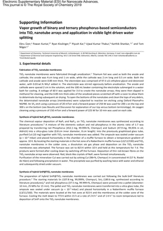
5. Figure S2. Selected point AES spectra on FIB-milled NaPx@TiO2 nanotube specimen. The according peaks at spot 1 (seeming hole) are P LVV (115 eV), C KLL
(266 eV), Ti LMM (381 eV, 416 eV), O KLL (482 eV, 503 eV), a weak peak at 979 eV potentially caused by Na KLL.
2. Results
NaP7@TiO2 nanotubes
P-XRD analysis
Figure S1. a) and b) Powder X-ray diffraction patterns of NaP7 (main fraction) and NaP15 (minor fraction) substantiate the formation of the two polyphosphides
on the membrane.
AES analysis
SnIP@TiO2 nanotubes

6. P-XRD analysis
Figure S3. Powder X-ray diffraction patterns confirm the formation of crystalline SnIP onto the membrane.
(CuI)3P12@TiO2 nanotubes
The gas-phase based synthesis was furthermore applied for the ternary polyphosphide (CuI)3P12. According to
calculations (CuI)3P12 and its structurally related compounds Cu2I3P3, and (CuI)2P14 show a band gap range of 1.0 -
1.1 eV.7 Downsizing quantum confinement effects such as in single and isolated phosphorus --strands
1
∞[𝑃10]𝑃2[
without the CuI-matrix lead to bandgaps of 2.3 - 2.9 eV.7 A growth of such isolated strands can be achieved by the
infiltration in hollow TiO2 nanotubes.
The polyphosphide substructure consists of condensed five- and six-membered ring fragments attached to a
polymer subunit in the CuI matrix.5 In line with Baudler’s rules the one-dimensional infinite phosphorus chains
in the (CuI)3P12 structure are more stable than the structurally related Cu2I3P3 with infinite chains
1
∞([𝑃10]𝑃2[)0
inhibiting additional four-membered rings.8-11 In Figure S4a the (CuI)3P12 - crystal structure consisting of
1
∞[𝑃 0
12]
separated CuI and polymeric phosphorus tubes along the b-axis is demonstrated. A microscopic image of the TiO2
nanotube membranes show the surface covered with dark blue fibres of (CuI)3P12 (Figure S4b). The SEM image in
Figure S4c confirms preservation of the nanotube structure after gas phase synthesis procedure as well as the
according elemental composition (Table S3). Powder X-ray diffraction verifies the growth of (CuI)3P12 on top of the
TiO2 nanotube membranes (Figure S4d).
Figure S4. a) Crystal structure of (CuI)3P12 with CuI and polymeric P units. b) A TiO2 nanotube membrane reacted with (CuI)3P12 via gas phase. c) Cross section and
surface of (CuI)3P12@TiO2 nanotube membranes. d) Powder X-ray diffraction patterns confirm the formation of crystalline (CuI)3P12 onto the membrane.
Raman imaging of the razor-cut cross section of hybrid (CuI)3P12@TiO2 nanotube membranes cutting demonstrates
the successful growth of (CuI)3P12 crystals up to 22 µm in distance to the membrane-top side (Figure S5).

7. Figure S5. Raman spectroscopy on (CuI)3P12@TiO2 membranes. a) Corresponding membrane cross section of measured specimen. b) From top to down:
Reference Raman spectrum of measured (CuI)3P12 crystals, spectra of a (CuI)3P12@TiO2 membrane cross section measured at approx. 22 μm in distance to the
surface (membrane-top side and a fresh TiO2 membrane (anatase, grey). c) A zoom in into the significant bands between 300 and 550 cm-1 of the (CuI)3P12 Raman
spectrum.
STEM images show a ranged bundle of non-decayed TiO2 nanotubes taken after separation by an ultrasonication
process. The image scale displays a size of ~90-100 nm per tube. An infiltration is shown by distribution of Ti and P
along, with Cu and I according to elemental mapping is illustrated along the tube length of the nanotube bundle
(see Figure S6a).
Figure S6. a) STEM bright-field image of TiO2 nanotubes separated from a membrane by an ultrasonication procedure. b) Elemental mapping of overlaid elements
Ti (representing TiO2), P, Cu and I. The elemental mapping images of c) Ti, d) P, e) Cu and f) I substantiating P, Cu and I distributed along the length of a TiO2
nanotube bundle.
XPS analysis
High resolution X-ray photoelectron spectroscopy (HR-XPS) was performed to investigate the surface chemical
composition, binding energy and oxidation state of the elements. XPS elemental survey scan of NaP7, TiO2 and
NaP7@TiO2 reveals the presence of all elements in NaP7 (Na1s, P2p), TiO2 (Ti2p, O1s) and NaP7@TiO2 (Na1s, P2p,
Ti2p, O1s) (Figure S7a). HR-XPS in Ti2p region for TiO2 reveal two peak components at BE ≈ 459.46 and 465.27 eV
assigned to Ti2P3/2 and Ti2p1/2 splitting, demonstrating presence of anatase form TiO2 with Ti4+ in crystal lattice
(Figure S7b).12 The peak position of Ti2P3/2 and Ti2p1/2 components does not change in hybrid NaP7@TiO2 suggesting
anatase phase TiO2 remains intact during deposition step. The deconvoluted HR-XPS spectra of TiO2 nanotubes in
O1s region shows two peak components at 530.98 and 532.70 eV. The strong peak at 530.98 eV was originated from
lattice oxygens bonded to Ti in crystal (Ti-O-Ti), while relatively weak shoulder peak at 532.70 eV was assigned to
non-lattice adventitious oxygen and surface –OH groups. Additionally, two peak components in O1s spectra
cantered at 530.98 and 532.70 eV for TiO2 remains unchanged in and NaP7@TiO2 which reveal robust nanotube

8. structure even after vapor phase deposition of NaP7 on TiO2 (Figure S7c).13 However, the increase in peak intensity
of 532.70 eV exhibit increase in adventitious oxygen which might be due to partial surface oxidation of phosphide
to various P-O moieties (PxOy). The peak positioned at 1063.74 eV in Na1s HR-XPS spectra for NaP7 originated from
electrostatically bonded Na+ to the phosphide backbone.14-17 Surprisingly, The Na1s peak in NaP7@TiO2 was shifted
to higher binding energy which might be due to partial charge transfer from NaP7 to the surface of TiO2 and partial
doping of TiO2 surface with Na ions (Figure S7d). Additionally, HR-XPS of NaP7 in P 2p region show two peaks centred
at BE ≈ 130.15 and 134.16 eV. The peak at 129.86 eV can be further deconvoluted into two peak components located
at BE≈129.90 and 130.77 eV and might have originated due to coexistence of two phases NaP7 (dominant fraction)
and NaP15 (both responsible for the 129.86 eV peak due to comparable polyphosphide substructures and
crystallographically non-equivalent P species)16, 17 The peak at 134.16 eV was originated due to partially oxidized
surfaces (phosphate formation, PxOy). A significant increase of the peak positioned at 130.15 eV appears in the
NaP7@TiO2 nanocomposite. The increase signal intensity might be due to a reduced oxidation tendency of the
polyphosphide in the hybrid (Figure S7e).
Figure S7. a) Elemental survey scan of TiO2 nanotube membranes (green), NaP7 (pink) and NaP7@TiO2 (navy blue) and HR-XPS spectra of TiO2 and NaP7@TiO2, b)
in Ti2p region, c) in O1s region, d) in Na1s region, e) in P2p region.
Like NaP7, the elemental survey scan of (CuI)3P12, TiO2 nanotube membrane and hybrid (CuI)3P12@TiO2 confirms
presence of all the relevant elements in (CuI)3P12 (Cu, I and P), TiO2 and (CuI)3P12@TiO2 (Cu, I, P, Ti and O) (Figure S8a).
The high resolution XPS (HR-XPS) core level spectra of TiO2 in Ti2p region can be deconvoluted into two peak
components located at binding energy 459.46 and 465.27 eV assigned to Ti2p3/2 and Ti2p1/2 components of Ti4+
oxidation state of anatase phase TiO2 (Figure S8b).18, 19 After solid state vapour phase deposition of (CuI)3P12 on TiO2
nanotube membranes ((CuI)3P12@TiO2) the binding energy of Ti2p3/2 and Ti2p1/2 components doesn’t change, which
confirms that the chemical nature of TiO2 doesn’t change during deposition of (CuI)3P12. The HR-XPS spectra of TiO2
in O1s region can be deconvoluted into two peak components at 530.48 and 532.64 eV. The origin of the stronger
peak at BE ≈ 530.48 eV was attributed to lattice oxygens (Ti-O-Ti), while smaller peak component located at
532.68 eV was originated due to presence of non-lattice adventitious oxygen and surface –OH groups (Figure S8c).20
For (CuI)3P12@TiO2, the binding energy of O1s peak components corresponding to lattice oxygen and adventitious
oxygens remains identical; however, the intensity of non-lattice bounded peak components are increased
significantly which might be due to the affinity of (CuI)3P12 to moisture and oxidation of surface phosphorous to

9. phosphates (PxOy). HR-XPS spectra of bare (CuI)3P12 in Cu2p region displayed two peak components at
BE ≈ 932.91 eV and 952.55 eV, attributed to Cu2p3/2 and Cu2p1/2 components of Cu present in the +1 oxidation state
(Figure S8d).21, 22 Furthermore, the absence of any shoulder peak in Cu2p XPS at higher binding energies confirms
the presence of Cu1+ atoms in identical chemical environment.23 The Cu2p HR-XPS remains the same for the hybrid
of (CuI)3P12@TiO2, which demonstrates successful solid-state deposition of (CuI)3P12 on TiO2 nanotubes. Two peak
components in HR-XPS scan in I3d region corresponded to I3d5/2 and I3d3/2 at BE of 631.42 and 619.94 eV show a
presence of I- coordinated to Cu1+ composing Cu-I-Cu bridges of polymeric structure (Figure S8e).24, 25 The binding
energy of the I3d peak component in (CuI)3P12@TiO2 gets shifted slightly to higher binding energy which might be
due to chemical interaction of outer coordinated iodine with electronegative oxygen of TiO2. Additionally, the single
peak component in P2p region (134.95 eV) of (CuI)3P12 might be originated due contribution from oxidized P atoms
present in the form of phosphate (PxOy) and the presence single phase Cu and iodine bonded phosphide chain
(Figure S8f).26, 27 However, considering high signal intensity we inferred phosphides were main contributor to this
signal. Further the peak located at 134.95 eV can be split into two peak components centred at 134.39 and 135.27
eV for 2p3/2 and 2p1/2 peak components. Similar to the I3d peak, the P2p peak component gets shifted to higher
binding energies due to the slight charge transfer from phosphorous helix to TiO2 surface.
Figure S8. a) Elemental survey scan of TiO2 nanotube membranes (orange), (CuI)3P12 (navy blue) and (CuI)3P12@TiO2 (green), HR-XPS core level spectra of TiO2
and (CuI)3P12@TiO2, b) in Ti2p region, c) in O1s region, and HR-XPS spectra of (CuI)3P12 and (CuI)3P12@TiO2 d) in Cu2p region, e) in I3d region and f) in P2p region.
(CuIP ⇒ (CuI)12P3).
The elemental survey scan of SnIP, TiO2 and SnIP@TiO2 displayed all peaks of composing elements present in SnIP
(Sn3d, I3d, P2p), TiO2 (Ti2p, O1s) and SnIP@TiO2 (Sn3d, I3d, P2p, Ti2p, O1s) (Figure S9a). The HR-XPS spectra of the
bare SnIP samples in Sn3d region displayed two deconvoluted peaks at 487.51 and 495.88 eV attributed to Sn3d5/2
and Sn3d3/2 components, revealing a presence of chemically equivalent Sn present in +2 oxidation state
(Figure S9b).28, 29 The HR-XPS spectra of SnIP showed two peak components at binding energies 619.87 and
631.37 eV in I3d region assigned to I3d5/2 and I3d3/2 peak component of I- composing the SnIP helix (Figure S9c).30, 31
Additionally, HR-XPS spectra of SnIP in P2p region show two peaks at 134.01 eV (deconvoluted into two components,
2p3/2-133.73 eV and 2p1/2-134.71 eV) for crystallographic non-equivalent P of SnIP and 139.77 eV (Phosphate,
surface oxidation product PxOy) (Figure S9d).32, 33 The binding energies corresponding to Sn2p, I3d and P2p peak
components remain fairly constant after fabrication of SnIP on TiO2 (SnIP@TiO2) which signify the absence of any
chemical interaction between SnIP and TiO2 (Figure S9b-d). The HR-XPS core level spectra in Ti2p region for TiO2

10. nanotubes displays two peak components at 466.43 and 465.23 eV assigned to Ti2p3/2 and Ti2p1/2, revealing the Ti4+
states in anatase TiO2 lattice (Figure S9e).34 The HR-XPS spectra in O1s region of TiO2 deconvoluted into two peak
components gave peak at BE≈ 531.86 and 532.74 eV corresponding to lattice bounded oxygen and adventitious
surface adsorbed oxygen (Figure S9f).35 After gas-phase deposition of SnIP on TiO2 nanotube membranes the signal
for Ti2p disappeared which was assumed due to coverage of TiO2 nanotube membrane with SnIP materials resulting
in suppression of the signals at the measured area (Figure S9e). While the O1s signal get slightly shifted to lower
binding energies (530.98 eV) and the peak component at 532.74 eV gets increased, showing some oxidation of SnIP
phosphorus to P-O (PxOy) functionalities and surface adsorbed adventitious oxygen.36
Figure S9. a) Elemental survey scan of TiO2 nanotube membranes (purple), SnIP (red) and SnIP@TiO2 (yellow) and HR-XPS core level spectra of TiO2
and SnIP@TiO2, b) in Sn3d region, c) in I3d region, d) in P2p region, e) in Ti2p region and f) in O1s region.

11. Diffuse reflectance spectroscopy
Figure S10. UV-Vis DRS spectra of a) TiO2 nanotubes (black),NaP7 (blue), NaP7@TiO2 (red), b) TiO2 (black), SnIP (blue), SnIP@TiO2 (red), c) TiO2 (black), (CuI)3P12
(blue), (CuI)3P12@TiO2 (red) and Tauc plot for determination of optical band gap of d) TiO2 (black), NaP7 (blue), NaP7@TiO2 (red) e) TiO2 (black), SnIP (blue),
SnIP@TiO2 (red), f) TiO2 (black), (CuI)3P12 (red), (CuI)3P12@TiO2 (blue). (CuIP ⇒ (CuI)12P3).

12. Figure S11. a) - l) Photocurrent density vs applied voltage plot with on-off cycles of TiO2 nanotubes vs NaP7, NaP7@TiO2, SnIP, SnIP@TiO2, (CuI)3P12, (CuI)3P12@TiO2.
(CuIP ⇒ (CuI)12P3).

13. a b c
d e f
Figure S12. a) – f) Photocurrent density vs applied voltage plot of TiO2 nanotubes, (CuI)3P12@TiO2, NaP7, NaP7@TiO2, SnIP and SnIP@TiO2 under the illumination
of LED 425 and 505 nm. (CuIP ⇒ (CuI)12P3).
Interface photon-to-current performance
Investigations on semiconductor/interface performance revealed following diagnostic efficiencies of the
materials.37, 38
Applied bias photon-to-current efficiency (ABPE):
The applied bias photon-to-current efficiency percentage (ABPE%) which demonstrates photo-conversion efficiency
under applied bias of the photoanode was determined by plotting a graph between ABPE% and applied voltage on
RHE (reversible hydrogen electrode) scale. The ABPE% was calculated by using following expression:
ABPE (%) = [J (mA cm–2) x (1.23–Vb)/ P (mW cm–2)] x 100
(1)
Where, J is the current density, Vb is the applied voltage at RHE scale and P is the power density of the incident light.
The applied voltage on Ag/AgCl scale was converted to RHE scale by using following expression.
VRHE = VAg/AgCl + 0.059 pH + V0
Ag/AgCl
(2)
Where = 0.197 V.
𝑉 0
𝐴𝑔/𝐴𝑔𝐶𝑙
Incident photon-to-current efficiency (IPCE) also referred as external quantum efficiency (EQE):
The IPCE which is a measure of the obtained photocurrent (number of electrons collected) per incident photon flux
as a function of wavelength was calculated at 0.6 V vs Ag/AgCl (1.23 V vs RHE, thermodynamic water splitting
potential) by irradiating samples with a 505 nm wavelength LED (40.48 mW cm–2). The IPCE values were calculated
using the following expression.
IPCE% = [1240 x J (mA cm–2)/λ (nm) x P (mW cm–2)] x 100
(3)
Where, J is the photocurrent density, λ is the wavelength of incident light in nm, and P is the power density of the
incident light.
Absorbed photon-to-current efficiency percentage (APCE%) also referred to as internal quantum efficiency (IQE):
Since IPCE is a measure to incident photons conversion efficiency, it doesn’t take the loss of photons being
unabsorbed by the materials into account. So, absorbed photon-to-current efficiency percentage (APCE%) which

14. define the photocurrent collected per incident photon absorbed is used to demonstrate device performances. The
APCE% can be calculated by following formulas:
APCE% = (IPCE/LHE) x 100
(4)
Where, LHE is the light harvesting efficiency or absorbance which is a number of electron-hole pairs produced as
fraction per incident photon flux. By considering that each absorbed photon produces equal electron hole pairs, the
value of LHE or absorptance calculated by Beer’s law can be expressed by following equation.
LHE or absorptance = (1-10-A)
APCE% = [1240 x J (mA cm–2)/λ (nm) x P (mW cm–2) x (1-10-A)] x 100
(5)
Where, J is photocurrent density, λ is wavelength of incident light in nm, P is the power density of incident light, LHE
is light harvesting efficiency and A is absorbance at measured wavelength.
Semiconductor-electrolyte interface
Electrochemical impedance spectroscopy
Semiconductor electrolyte interfacial (SEI) behaviour of NaP7 and NaP7@TiO2, SnIP, SnIP@TiO2, (CuI)3P12,
(CuI)3P12@TiO2 were analysed using electrochemical impedance spectroscopy (EIS), whereby Nyquist plots
were obtained, between frequencies of 1 and 10,000 Hz at -0.4 V vs Ag/AgCl, using dark and one-sun conditions. EIS
Nyquist plots (Figure S13a, b and c) clearly indicate higher charge transfer resistance in dark conditions when
compared to those in one-sun illumination condition. Equivalent circuit diagram representing the Nyquist plots is
shown in Figure S13d, wherein in RS, RC, RT, CSC, and CH are electrolyte resistance, charge transfer resistance, charge
transport resistance, space charge capacitance, and electrochemical double-layer (Helmholtz) capacitance,
respectively. Q is a constant phase element with coefficient n. The values of circuit parameters are listed in Table
S4. As obtained by equivalent circuit model, RC was the same (i.e. 10 ohms) (CuI)3P12 and SnIP, as it was (i.e. 1 ohm)
for SnIP@TiO2 and NaP7@TiO2. RC for (CuI)3P12@TiO2 and NaP7 were rather high at 50 and 30 ohms, respectively.
Calculated recombination lifetime ( , using (6) values are listed in Table S5, and indicate reasonably long-lived holes
𝜏
for all samples, and particularly for SnIP and NaP7.
Figure S13. Nyquist plots measured in 0.1 M KOH, under dark conditions and AM1.5 G light irradiation (100 mW cm−2) a) TiO2 nanotubes (black and magenta),
NaP7 (light and dark blue), NaP7@TiO2 (light and dark red), b) TiO2 (black and magenta), SnIP (dark and light green), SnIP@TiO2 (light and dark red), c) TiO2 (black
and magenta), (CuI)3P12 (light and dark blue), (CuI)3P12@TiO2 (light and dark red). d) Equivalent circuit diagram of the EIS Nyquist plots shown in a, b and c. (CuIP
⇒ (CuI)12P3).
𝜏 = 𝑅𝑇𝐶𝑆
𝐶
(6)
1
𝐶 2
𝑆
𝐶
=
2
𝑒
𝜀 0𝜀𝑟𝑁𝐷
{(𝑉 ‒ 𝑉𝐹
𝐵 ) ‒
𝑘
𝑇
𝑒 }
(7)
𝑁𝐷 =
2
𝑒
𝜀 0𝜀𝑟
{
𝑑𝑉
𝑑𝐶 2
𝑆
𝐶
}
(8)

15. 𝑊 = {
2𝜑𝜀0𝜀𝑟
𝑒𝑁𝐷
}0
.
5
(9)
Impedance-potential analysis
Further insights about SEI of the samples were gained via Mott Schottky’s equations (eq. (7) and (8)), which were
used to calculate charge carrier concentration ( ), and flat band potential ( ). In eq. (7) and (8), CSC is space-
𝑁𝐷 𝑉𝐹𝐵
charge capacitance per unit area; the dielectric constant of the samples, which may be assumed to be 45, i.e.
𝜀𝑟
same as that of anatase TiO2.39, 40 is carrier concentration; is the vacuum permittivity (8.854 ×10−14 F cm−1);
𝑁𝐷 𝜀0 𝑘
is the Boltzmann constant (1.381 ×10−23 J K−1); T is the temperature in (298 K); e is the electron charge
(1.602×10−19 C); is the flat band potential; and V is the applied potential. , the charge carrier concentration,
𝑉𝐹𝐵 𝑁𝐷
is calculated from the slope (term within the bracket in eq. (8) of the Mott Schottky’s plots (Figure S14), using eq. (8).
, is the point of intersection of the slope of the Mott Schottky’s plot with the potential axis, as shown in Figure
𝑉𝐹𝐵
S14. and of the samples are listed in Table S5. of the order of 1020 cm-3, is well known for anatase TiO2
41
𝑁𝐷 𝑉𝐹𝐵 𝑁𝐷
of the composites of (CuI)3P12 and SnIP with TiO2 decreased, as it did for bare (CuI)3P12 and SnIP, while that of
𝑁𝐷
NaP7@TiO2 increased slightly from bare TiO2 nanotube arrays, while that for bare NaP7 decreased slightly. Width of
depletion layer, W, is calculated using eq. (9) at 1.23 V vs RHE in eq. (9), where is the potential drop across the
𝜑
space layer. W is highest for SnIP and SnIP@TiO2 indicating maximum band bending in those samples due to the
lower carrier concentration.
Figure S14. Mott-Schottky plots, linear fit of plot intersecting on abscissa reveal flat band potential of a) TiO2 nanotubes (black), NaP7 (blue), NaP7@TiO2 (red), b)
TiO2 (black), SnIP (blue), SnIP@TiO2 (red), c) TiO2 (black), (CuI)3P12 (blue), (CuI)3P12@TiO2 (red) in 0.5 M Na2SO4. (CuIP ⇒ (CuI)12P3).
Figure S15. XPS valance band spectra of TiO2 nanotube membranes showing the position of valance band maxima (VBmax) below Fermi level.
Kelvin Probe Force Microscopy (KPFM) Mesurement
To understand the dynamics of charge carrier separation and probe heterojunction formation between
polyphosphides and TiO2, surface potential (SP) difference of materials was determined using Kelvin Probe Force

16. Microscopy (KPFM) (Figure S16). The AFM topographical images of the samples displayed rough morphology and
evidential presence of nanotube arrays (Figure S16a-d). The surface potential (SP) map of bare TiO2, NaP7@TiO2,
CuIP@TiO2 and SnIP@TiO2 deposited on FTO under dark condition is displayed in Figure S16a-d. The surface
potential map of the samples shows uniform charge distribution at all sample surfaces. For bare TiO2 nanotubes
some bright region was observed which demonstrates electron rich surface of n-type TiO2 nanotubes. Furthermore,
the surface potential map contrast of SnIP@TiO2 sample was slightly higher than other hybrid materials (NaP7@TiO2
and CuIP@TiO2) which demonstrates higher electronic density of these materials. The surface potential distribution
of bare TiO2 was found to be ~38 mV, while SP of polyphosphide@TiO2 hybrids, NaP7@TiO2, CuIP@TiO2 and
SnIP@TiO2 was calculated to be ~ 27, 26, and 31 mV. A slightly negative shift of SP distribution of hybrid samples
was corroborated to the lowering of work function value of nanohybrids. The lowering of WF (work function) value
is attributed to the uplifting of the Fermi level of polyphosphides during Fermi level alignment in heterojunction
formation because of charge carrier gradients (in-built electric field). The evident change in WF values and band
structure clearly suggests successful formation of heterojunction between the materials.
Figure S16. Topographical AFM images and surface potential map of a) TiO2 nanotube, b) NaP7@TiO2, c) (CuI)3P12@TiO2, d) SnIP@TiO2 and e) surface potential
distribution of bare TiO2 nanotubes (black), NaP7@TiO2 (red), (CuI)3P12@TiO2 (blue) and SnIP@TiO2 (green) samples deposited on FTO under dark conditions.
Figure S17. Left side: Plausible mechanism of charge separation in inorganic phosphides@TiO2 heterojunction. Right side: Hybrid materials including
heterojunction formation between TiO2 nanotubes and different polyphosphides (NaP7, SnIP and (CuI)3P12) for PEC-water-oxidation. (CuIP ⇒ (CuI)12P3).

17. EDS analysis
Table S1. Elemental analysis of deposited crystals found on both sides of the membranes and different spots along the razor cut cross section of NaPx@TiO2
membranes via EDS-measurements. Elemental composition in at.% with corresponding molar ratio deriving from the Na and P content and normalized to the Na
content. Atomic percent of Ti is representing Ti in TiO2.
EDS - NaPx Na (at%) P (at%) Ti (at%)
NaP7 12.5 87.5 NaP7
NaP15 6.25 93.75 NaP15
NaP7 measured, crystal 12.0(4) 87.9(1) - Na0.96P7.03
NaP15 measured, crystal 5.6(8) 94.4(2) - Na0.9P15.1
NaPx@TiO2 cross section 1 3.6(2) 16.4(2) 80.1(2) NaP4.5
NaPx@TiO2 cross section 2 1.5(1) 13.5(1) 85.0(3) NaP9
Table S2. Elemental analysis of deposited crystals found on both sides of the membranes and different spots along the razor cut cross section of SnIP@TiO2
membranes via EDS-measurements. Elemental composition in at% with corresponding molar ratio deriving from the Sn, I and P content and normalized to the P
content. Atomic percent of Ti is representing Ti in TiO2.
EDS - SnIP Sn (at%) I (a%) P (at%) Ti (at%)
SnIP 1 1 1 SnIP
SnIP measured, crystal 37.8(3) 26.3(3) 35.7(1) - SnI0.7P
SnIP@TiO2 cross section 1 13.2(2) 9.4(2) 20.2(2) 57.1(4) SnI0.7P
SnIP@TiO2 cross section 2 10.5(6) 7.4(4) 18.6(8) 63.5(2) Sn0.6I0.4P
Table S3. Elemental analysis of deposited crystals found on both sides of the membranes and different spots along the razor cut cross section of (CuI)3P12@TiO2
membranes via EDS-measurements. Elemental composition in at% with corresponding molar ratio deriving from the Cu, I and P content and normalized to the P
content. Atomic percent of Ti is representing Ti in TiO2.
EDS - (CuI)3P12 Cu (at%) I (at%) P (at%) Ti (at%)
CuI)3P12 16.67 16.67 66.67 Cu3I3P12
(CuI)3P12 measured, crystal 14.7(4) 16.1(3) 69.1(3) - Cu2.6I2.8P12
(CuI)3P12@TiO2 cross section 1 2.4(3) 2.5(3) 24.5(3) 72.6(5) Cu1.2I1.2P12
(CuI)3P12@TiO2 cross section 2 16.5(5) 13.2(6) 69.0(5) 73.0(8) Cu2.9I2.3P12

18. Electrochemical impedance spectroscopy and impedance-potential analysis
Table S4. Values of electrolyte resistance RS, charge transfer resistance RC, charge transport resistance RT, space charge capacitance CSC, electrochemical double-
layer (Helmholtz) capacitance CH and constant phase element Q with coefficient n for (CuI)3P12, (CuI)3P12@TiO2, SnIP, SnIP@TiO2, NaP7, NaP7@TiO2, obtained by
fitting the Nyquist plots to the equivalent circuit (Figure S13).
Sample RS (Ohm) CSC (F) RT (Ohm) CH (F) RC (Ohm) Q (Fs-1 + n) n
(CuI)3P12 16 9.00x10-8 21 1.25x10-5 10 5.50x10-4 0.35
(CuI)3P12@TiO2 16 6.00x10-8 31 1.85x10-5 50 5.80x10-4 0.39
SnIP 16 1.00x10-7 30 1.00x10-5 10 4.75x10-4 0.45
SnIP@TiO2 16 1.10x10-7 22 6.00x10-6 1 9.50x10-4 0.50
NaP7 16 2.00x10-7 16 1.50x10-5 30 2.00x10-4 0.54
NaP7@TiO2 16 8.50x10-8 22 1.50x10-5 1 2.10x10-4 0.52
Table S5. Values of charge carrier concentration , flat band potential , width of depletion layer W and calculated recombination lifetime τ for (CuI)3P12,
𝑁𝐷 𝑉𝐹
𝐵
(CuI)3P12@TiO2, SnIP, SnIP@TiO2, NaP7, NaP7@TiO2 and TiO2, obtained by fitting the Nyquist plots to the equivalent circuit (Figure S13).
Sample ND (cm-3) VFB
(V vs Ag/AgCl)
VFB
(V vs NHE at pH-0)
W (nm) τ (µs)
(CuI)3P12 3.88x1020 -0.721 -0.522 113.18 1.90
(CuI)3P12@TiO2 3.83x1020 -0.692 -0.493 157.14 1.90
SnIP 1.69x1020 -0.730 -0.531 712.80 3.00
SnIP@TiO2 1.05x1020 -1.930 -1.731 922.89 2.40
NaP7 4.75x1020 -0.670 -0.471 376.09 3.20
NaP7@TiO2 5.62x1020 -0.780 -0.581 118.95 1.90
TiO2 5.05x1020 -0.702 -0.503 197.42 -
Table S6. Binding energies of different element and species present in TiO2 nanotubes, NaP7, NaP7@TiO2, (CuI)3P12, (CuI)3P12@TiO2, SnIP, SnIP@TiO2.
Sample Ti2p
(Ti2p3/2)
(Ti2p1/2)
O1s
(Olatt.)
(-OH)
Na1s
(Na1s)
Cu2p
(Cu 2p3/2)
(Cu2p1/2)
Sn3d
(Sn3d5/2)
(Sn3d3/2)
I3d
(I3d5/2)
(I3d3/2)
P2p
(P2p3/2)
(P2p1/2)
(PxOy)
TiO2 459.46
465.27
530.98
532.70
- -
-
-
-
-
-
-
-
-
NaP7 -
-
-
-
1063.74 -
-
-
-
- 129.90
130.77
134.56
NaP7@TiO2 459.46
465.27
530.98
532.70
1071.83 -
-
-
-
- 130.00
130.98
133.82
(CuI)3P12 -
-
-
-
- 932.91
952.55
-
-
619.94
631.42
134.39
135.27
-
(CuI)3P12@TiO2 459.46
465.27
530.48
532.64
- 932.91
952.55
-
-
620.30
631.89
134.40
135.33
-
SnIP -
-
-
-
- -
-
487.51
495.88
619.87
631.37
133.73
134.71
139.77
SnIP@TiO2 -
-
530.98
532.74
- -
-
487.51
495.88
619.87
631.37
133.94
134.83
139.77
All binding energy values are in eV.

19. References
1. G. K. Mor, K. Shankar, M. Paulose, O. K. Varghese and C. A. Grimes, Nano Lett., 2006, 6, 215-218.
2. C. Grotz, M. Köpf, M. Baumgartner, L. A. Jantke, G. Raudaschl-Sieber, T. F. Fässler and T. Nilges, Z. Anorg. Allg. Chem.,
2015, 641, 1395-1399.
3. D. Pfister, K. Schaefer, C. Ott, B. Gerke, R. Poettgen, O. Janka, M. Baumgartner, A. Efimova, A. Hohmann, P. Schmidt, S.
Venkatachalam, L. van Wuellen, U. Schuermann, L. Kienle, V. Duppel, E. Parzinger, B. Miller, J. Becker, A. Holleitner, R.
Weihrich and T. Nilges, Adv. Mater. (Weinheim, Ger.), 2016, 28, 9783-9791.
4. W. G. Palmer, Experimental inorganic chemistry, Cambridge University Press, Cambridge, 1962.
5. A. Pfitzner and E. Freudenthaler, Angew. Chem. Int. Ed., 1995, 34, 1647-1649.
6. U. K. Thakur, A. M. Askar, R. Kisslinger, B. D. Wiltshire, P. Kar and K. Shankar, Nanotechnology, 2017, 28, 274001.
7. M. P. Baumgartner, Technische Universität München, 2017.
8. M. Baudler, Angew. Chem., 1982, 94, 520-539.
9. M. Baudler, Angew. Chem., 1987, 99, 429-451.
10. M. Baudler and K. Glinka, Chem. Rev., 1993, 93, 1623-1667.
11. S. Böcker and M. Häser, Z. Anorg. Allg. Chem., 1995, 621, 258-286.
12. G. Yang, D. Chen, H. Ding, J. Feng, J. Z. Zhang, Y. Zhu, S. Hamid and D. W. Bahnemann, Appl. Catal. B, 2017, 219, 611-
618.
13. M. Wang, B. Nie, K.-K. Yee, H. Bian, C. Lee, H. K. Lee, B. Zheng, J. Lu, L. Luo and Y. Y. Li, Chem. Commun., 2016, 52,
2988-2991.
14. W.-J. Kwak, Z. Chen, C. S. Yoon, J.-K. Lee, K. Amine and Y.-K. Sun, Nano Energy, 2015, 12, 123-130.
15. T. Kajita and T. Itoh, Phys. Chem. Chem. Phys., 2018, 20, 2188-2195.
16. J. Song, C. Zhu, B. Z. Xu, S. Fu, M. H. Engelhard, R. Ye, D. Du, S. P. Beckman and Y. Lin, Adv. Energy Mater., 2017, 7,
1601555.
17. X. Zhong, Y. Jiang, X. Chen, L. Wang, G. Zhuang, X. Li and J.-g. Wang, J. Mater. Chem. A, 2016, 4, 10575-10584.
18. Y. Zhou, C. Chen, N. Wang, Y. Li and H. Ding, J. Phys. Chem. C, 2016, 120, 6116-6124.
19. R. Kumar, S. Govindarajan, R. K. Siri Kiran Janardhana, T. N. Rao, S. V. Joshi and S. Anandan, ACS Appl. Mater.
Interfaces, 2016, 8, 27642-27653.
20. F. Amano, M. Nakata, A. Yamamoto and T. Tanaka, J. Phys. Chem. C, 2016, 120, 6467-6474.
21. I.-H. Tseng, W.-C. Chang and J. C. Wu, Appl. Catal., B, 2002, 37, 37-48.
22. C. S. Chen, A. D. Handoko, J. H. Wan, L. Ma, D. Ren and B. S. Yeo, Catal. Sci. Technol., 2015, 5, 161-168.
23. C. S. Chen, J. H. Wan and B. S. Yeo, J. Phys. Chem. C, 2015, 119, 26875-26882.
24. D. S. Bhachu, S. J. Moniz, S. Sathasivam, D. O. Scanlon, A. Walsh, S. M. Bawaked, M. Mokhtar, A. Y. Obaid, I. P. Parkin
and J. Tang, Chem. Sci., 2016, 7, 4832-4841.
25. M. J. Islam, D. A. Reddy, N. S. Han, J. Choi, J. K. Song and T. K. Kim, Phys. Chem. Chem. Phys., 2016, 18, 24984-24993.
26. D. Hanlon, C. Backes, E. Doherty, C. S. Cucinotta, N. C. Berner, C. Boland, K. Lee, A. Harvey, P. Lynch and Z.
Gholamvand, Nat. Commun., 2015, 6, 8563.
27. Z. Niu, J. Jiang and L. Ai, Electrochem. Commun., 2015, 56, 56-60.
28. G. G. Ninan, C. S. Kartha and K. Vijayakumar, Sol. Energy Mater. Sol. Cells, 2016, 157, 229-233.
29. W. Gao, K. Zielinski, B. N. Drury, A. D. Carl and R. L. Grimm, J. Phys. Chem. C, 2018, 122, 17882-17894.
30. M. Yan, Y. Hua, F. Zhu, W. Gu, J. Jiang, H. Shen and W. Shi, Appl. Catal. B, 2017, 202, 518-527.
31. J. C.-R. Ke, D. J. Lewis, A. S. Walton, B. F. Spencer, P. O'Brien, A. G. Thomas and W. R. Flavell, J. Mater. Chem. A, 2018.
32. X.-D. Wang, Y.-F. Xu, H.-S. Rao, W.-J. Xu, H.-Y. Chen, W.-X. Zhang, D.-B. Kuang and C.-Y. Su, Energy Environ. Sci., 2016,
9, 1468-1475.
33. H. Tabassum, W. Guo, W. Meng, A. Mahmood, R. Zhao, Q. Wang and R. Zou, Adv. Energy Mater., 2017, 7, 1601671.
34. S. G. Ullattil and P. Periyat, J. Mater. Chem. A, 2016, 4, 5854-5858.
35. H. Zhao, M. Wu, J. Liu, Z. Deng, Y. Li and B.-L. Su, Appl. Catal. B, 2016, 184, 182-190.
36. M. S. Milien, U. Tottempudi, M. Son, M. Ue and B. L. Lucht, J. Electrochem. Soc., 2016, 163, A1369-A1372.
37. Z. Chen, H. N. Dinh and E. Miller, Photoelectrochemical water splitting, Springer, 2013.
38. X. Zhang, B. Zhang, K. Cao, J. Brillet, J. Chen, M. Wang and Y. Shen, J. Mater. Chem. A, 2015, 3, 21630-21636.
39. H. Wang, Y. Liang, L. Liu, J. Hu and W. Cui, J. Hazard. Mater., 2018, 344, 369-380.
40. A. Muñoz, Q. Chen and P. Schmuki, J. Solid State Electrochem., 2007, 11, 1077-1084.
41. F. Y. Oliva, L. a. B. Avalle, E. Santos and O. R. Cámara, J. Photochem. Photobiol., A, 2002, 146, 175-188.