Este documento presenta notas de clase sobre mecánica cuántica. Contiene una introducción a los espacios vectoriales lineales y sus propiedades, incluyendo subespacios vectoriales, bases y dimensiones. También cubre espacios de Hilbert, operadores normales y autoadjuntos, y la notación de Dirac para representar vectores y operadores cuánticos. El documento proporciona una base sólida para comprender los fundamentos matemáticos de la mecánica cuántica.

![ÍNDICE GENERAL 13
26.10.2.Estado base de un sistema de partı́culas idénticas independientes . . . . . . . . . . . . . . . 611
26.11.
Predicciones fı́sicas del postulado de simetrización . . . . . . . . . . . . . . . . . . . . . . . . . . . 613
26.11.1.Predicciones sobre partı́culas aparentemente idénticas . . . . . . . . . . . . . . . . . . . . . 615
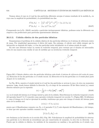
26.11.2.Colisión elástica de dos partı́culas idénticas . . . . . . . . . . . . . . . . . . . . . . . . . . . 616
26.12.
Situaciones en las cuales se puede ignorar el postulado de simetrización . . . . . . . . . . . . . . . 617
26.12.1.Partı́culas idénticas ubicadas en regiones espaciales distintas . . . . . . . . . . . . . . . . . . 617
26.12.2.Identificación de partı́culas por su dirección de espı́n . . . . . . . . . . . . . . . . . . . . . . 619
27.Átomos de muchos electrones y aproximación de campo central 620
27.1. Aproximación de campo central . . . . . . . . . . . . . . . . . . . . . . . . . . . . . . . . . . . . . . 621
27.2. Configuraciones electrónicas de los átomos . . . . . . . . . . . . . . . . . . . . . . . . . . . . . . . . 624
28.El átomo de Helio 626
28.1. Configuraciones del átomo de Helio . . . . . . . . . . . . . . . . . . . . . . . . . . . . . . . . . . . . 626
28.1.1. Degeneración de las configuraciones . . . . . . . . . . . . . . . . . . . . . . . . . . . . . . . 627
28.2. Efecto de la repulsión electrostática . . . . . . . . . . . . . . . . . . . . . . . . . . . . . . . . . . . . 629
28.2.1. Base de E (n, l; n′, l′) adaptada a las simetrı́as de W . . . . . . . . . . . . . . . . . . . . . . 629
28.2.2. Restricciones impuestas por el postulado de simetrización . . . . . . . . . . . . . . . . . . . 631
28.2.3. Términos espectrales generados por la repulsión electrostática . . . . . . . . . . . . . . . . . 633
28.3. Términos espectrales que surgen de la configuración 1s, 2s . . . . . . . . . . . . . . . . . . . . . . . 634
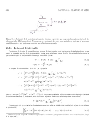
28.3.1. La integral de intercambio . . . . . . . . . . . . . . . . . . . . . . . . . . . . . . . . . . . . . 636
28.3.2. Análisis del papel del postulado de simetrización . . . . . . . . . . . . . . . . . . . . . . . . 637
28.3.3. Hamiltoniano efectivo dependiente del espı́n . . . . . . . . . . . . . . . . . . . . . . . . . . . 638
28.4. Términos espectrales que surgen de otras configuraciones excitadas . . . . . . . . . . . . . . . . . . 640
28.5. Validez del tratamiento perturbativo . . . . . . . . . . . . . . . . . . . . . . . . . . . . . . . . . . . 640
28.6. Estructura fina del átomo de helio y multipletes . . . . . . . . . . . . . . . . . . . . . . . . . . . . . 641
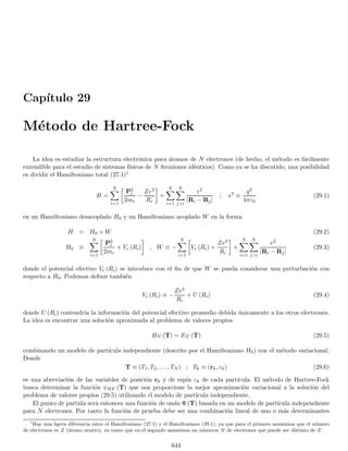
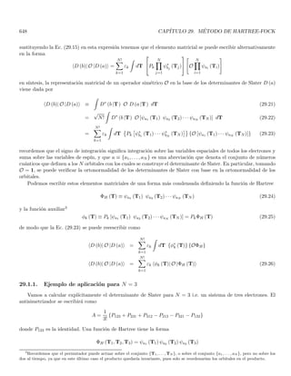
29.Método de Hartree-Fock 644
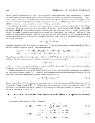
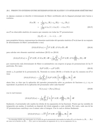
29.1. Producto interno entre determinantes de Slater y un operador simétrico . . . . . . . . . . . . . . . 646
29.1.1. Ejemplo de aplicación para N = 3 . . . . . . . . . . . . . . . . . . . . . . . . . . . . . . . . 648
29.2. Valor esperado de la energı́a . . . . . . . . . . . . . . . . . . . . . . . . . . . . . . . . . . . . . . . . 649
29.2.1. Valor esperado de H(0) . . . . . . . . . . . . . . . . . . . . . . . . . . . . . . . . . . . . . . . 650
29.2.2. Valor esperado de H(1) . . . . . . . . . . . . . . . . . . . . . . . . . . . . . . . . . . . . . . . 651
29.2.3. Valor esperado de H = H(0) + H(1) . . . . . . . . . . . . . . . . . . . . . . . . . . . . . . . . 653
29.2.4. Interpretación fı́sica de los términos directo y de intercambio . . . . . . . . . . . . . . . . . 653
29.3. Método de Hartree-Fock para una capa cerrada . . . . . . . . . . . . . . . . . . . . . . . . . . . . . 654
29.3.1. Minimización de E [D] con ligaduras . . . . . . . . . . . . . . . . . . . . . . . . . . . . . . . 655
29.3.2. Cálculo de δF [ψ, ψ∗
] . . . . . . . . . . . . . . . . . . . . . . . . . . . . . . . . . . . . . . . 656
29.4. Operadores de Hartree-Fock . . . . . . . . . . . . . . . . . . . . . . . . . . . . . . . . . . . . . . . . 658
29.5. Interpretación de la ecuación de Hartree-Fock . . . . . . . . . . . . . . . . . . . . . . . . . . . . . . 659
29.6. Solución por iteración de la ecuación de HF . . . . . . . . . . . . . . . . . . . . . . . . . . . . . . . 659
29.7. Determinación del valor Fı́sico de la energı́a . . . . . . . . . . . . . . . . . . . . . . . . . . . . . . . 660](https://image.slidesharecdn.com/cuantica-220626164623-64979fb3/85/cuantica-pdf-13-320.jpg)
![1.2. ALGEBRAIC PROPERTIES 15
Example 1.2 The set Rn (Cn) of all n-tuples of real (complex) numbers is a real (complex) linear space under
the following linear operations
x ≡ (x1, x2, . . . , xn) ; y ≡ (y1, y2, . . . , yn)
αx ≡ (αx1, αx2, , αxn) ; x + y ≡ (x1 + y1, x2 + y2, . . . , xn + yn)
Example 1.3 The set of all bounded continuous real functions defined on a given interval [a, b] of the real line,
with the linear operations defined pointwise as
(f + g) (x) = f (x) + g (x) ; (αf) (x) = αf (x) ; x ∈ [a, b]
We can see that a linear or vector space forms an abelian group whose elements are the vectors, and with
addition as the law of combination. However, the vector space introduce an additional structure by considering
multiplication by scalars which is not a group property.
Some very important kinds of vector spaces are the ones containing certain sets of functions with some specific
properties. We can consider for example, the set of functions defined on certain interval with some condition of
continuity integrability etc. For instance, in quantum mechanics we use a vector space of functions.
1.2. Algebraic properties
Some algebraic properties arise from the axioms:
The origin or identity 0 must be unique. Assuming another identity 0′ we have that x + 0′ = 0′ + x = x for
all x ∈ V. Then 0′ = 0′ + 0 = 0. Hence 0′ = 0.
The additive inverse of any vector x is unique. Assume that x′ is another inverse of x then
x′
= x′
+ 0 = x′
+ (x+ (−x)) = x′
+ x
+ (−x) = 0 + (−x) = −x
⇒ x′
= −x
xi + xk = xj + xk ⇒ xi = xj to see it, we simply add −xk on both sides. This property is usually called the
rearrangement lemma.
α · 0 = 0 we see it from α · 0 + αx = α · (0 + x) = αx = 0 + αx and applying the rearrangement lemma.
0 · x = 0 it proceeds from 0 · x + αx = (0 + α) x = αx = 0 + αx and using the rearrangement lemma.
(−1) x = −x we see it from x+ (−1) x = 1 · x + (−1) x = (1 + (−1)) x = 0x = 0 = x+ (−x) and the
rearrangement lemma.
αx = 0 then α = 0 or x = 0; for if α 6= 0 we can multiply both sides of the equation by α−1 to give
α−1 (αx) = α−10 ⇒ α−1α
x = 0 ⇒ 1x = 0 ⇒ x = 0. If x 6= 0 we prove that α = 0 by assuming α 6= 0 and
finding a contradiction. This is inmediate from the above procedure that shows that starting with α 6= 0 we arrive
to x = 0.
It is customary to simplify the notation in x+(−y) and write it as x−y. The operation is called substraction.
1.3. Vector subspaces
Definition 1.1 A non-empty subset M of V is a vector subspace of V if M is a vector space on its own right
with respect to the linear operations defined in V .
This is equivalent to the condition that M contains all sums, negatives and scalar multiples. The other pro-
perties are derived directly from the superset V . Further, since −x = (−1) x it reduces to say that M must be
closed under addition and scalar multiplication.
When M is a proper subset of V it is called a proper subspace of V . The zero space {0} and the full space V
itself are trivial subspaces of V .
The following concept is useful to study the structure of vector subspaces of a given vector space,](https://image.slidesharecdn.com/cuantica-220626164623-64979fb3/85/cuantica-pdf-15-320.jpg)
![16 CAPÍTULO 1. LINEAR OR VECTOR SPACES
Definition 1.2 Let S = {x1, .., xn} be a non-empty finite subset of V , then the vector
x = α1x1 + α2x2 + . . . + αnxn (1.1)
is called a linear combination of the vectors in S.
We can redefine a vector subspace by saying that a non-empty subset M of V is a linear subspace if it is closed
under the formation of linear combinations. If S is a subset of V we can see that the set of all linear combinations
of vectors in S is a vector subspace of V , we denote this subspace as [S] and call it the vector subspace spanned by
S. It is clear that [S] is the smallest subspace of V that contains S. Similarly, for a given subspace M a non-empty
subset S of M is said to span M if [S] = M. Note that the closure of a vector space under an arbitrary linear
combination can be proved by induction from the closure property of vector spaces under linear operations. Notice
additionally, that the proof of induction only guarantees the closure under any finite sum of terms, if we have an
infinite sum of terms (e.g. a series) we cannot ensure that the result is an element of the space, this is the reason
to define linear combinations as finite sums. If we want a property of closure under some infinite sums additional
structure should be added as we shall see later.
Suppose now that M and N are subspaces of V . Consider the set M + N of all sums of the form x + y with
x ∈ M and y ∈ N. Since M and N are subspaces, this sum is the subspace spanned by the union of both subspaces
M + N = [M ∪ N]. It could happen that M + N = V in this case we say that V is the sum of M and N. In turn
it means that every vector in V is expressible as a sum of a vector in M plus a vector in N. Further, in some cases
any element z of V is expressible in a unique way as such a sum, in this case we say that V is the direct sum of
M and N and it is denoted by
V = M ⊕ N
we shall establish the conditions for a sum to become a direct sum
Theorem 1.1 Let a vector space V be the sum of two of its subspaces V = M +N. Then V = M ⊕N ⇔ M ∩N =
{0}
Proof: Assume first that V = M ⊕ N, we shall suppose that ∃ z 6= 0 with z ∈ M ∩ N, and deduce a
contradiction from it. We can express z in two different ways z = z + 0 with z ∈ M and 0 ∈ N or z = 0 + z with
0 ∈ M and z ∈ N. This contradicts the definition of a direct sum.
Now assume M ∩ N = {0}, by hypothesis V = M + N so that any z ∈ V can be expressed by z = x1 + y1
with x1 ∈ M and y1 ∈ N. Suppose that there is another decomposition z = x2 + y2 with x2 ∈ M and y2 ∈ N.
Hence x1 + y1 = x2 + y2 ⇒ x1 − x2 = y1 − y2; but x1 − x2 ∈ M and y1 − y2 ∈ N. Since they are equal, then both
belong to the intersection so x1 − x2 = y1 − y2 = 0 then x1 = x2 and y1 = y2 showing that the decomposition
must be unique. QED.
When two vector subspaces of a given space have only the zero vector in common, it is customary to call them
disjoint subspaces. It is understood that it does not correspond to disjointness in the set-theoretical sense, after all
two subspaces of a given space cannot be disjoint as sets, since any subspace must contain 0. Thus no confusion
arises from this practice.
The concept of direct sum can be generalized when more subspaces are involved. We say that V is the direct
sum of a collection of subspaces {M1, .., Mn} and denote it as
V = M1 ⊕ M2 ⊕ . . . ⊕ Mn
when each z ∈ V can be expressed uniquely in the form
z = x1 + x2 + . . . + xn ; xi ∈ Mi
In this case if V = M1 +..+Mn, this sum becomes a direct sum if and only if each Mi is disjoint from the subspace
spanned by the others. To see it, it is enough to realize that
V = M1 + M2 + .. + Mn = M1 + [M2 + .. + Mn] = M1 + [∪n
i=2Mi]](https://image.slidesharecdn.com/cuantica-220626164623-64979fb3/85/cuantica-pdf-16-320.jpg)
![1.4. DIMENSION AND BASES IN VECTOR SPACES 17
then V = M1 ⊕ [M2 + .. + Mn] if and only if M1 ∩ [∪n
i=2Mi] = {0}, proceeding similarly for the other M′
is we
arrive at the condition above. Note that this condition is stronger than the condition that any given Mi is disjoint
from each of the others.
The previous facts can be illustrated by a simple example. The most general non-zero proper subspaces of R3
are lines or planes that passes through the origin. Thus let us define
M1 = {(x1, 0, 0)} , M2 = {(0, x2, 0)} , M3 = {(0, 0, x3)}
M4 = {(0, x2, x3)} , M5 = {(x1, 0, x3)} , M6 = {(x1, x2, 0)}
M1, M2, M3 are the coordinate axes of R3 and M4, M5, M6 are its coordinate planes. R3 can be expressed by direct
sums of these spaces in several ways
R3
= M1 ⊕ M2 ⊕ M3 = M1 ⊕ M4 = M2 ⊕ M5 = M3 ⊕ M6
for the case of R3 = M1⊕M2⊕M3 we see that the subspace spanned by M2 and M3 i.e. M2+M3 = [M2 ∪ M3] = M4
is disjoint from M1. Similarly M2 ∩[M1 ∪ M3] = {0} = M3 ∩[M1 ∪ M2]. It is because of this, that we have a direct
sum.
Now let us take M3, M6 and M′ defined as a line on the plane M4 that passes through the origin making an
angle θ with the axis x3 such that 0 θ π/2, since R3 = M3 + M6 it is clear that
R3
= M3 + M6 + M′
; M3 ∩ M6 = M3 ∩ M′
= M6 ∩ M′
= {0} (1.2)
however this is not a direct sum because M3 + M6 = R3 so that M′ ∩ (M3 + M6) 6= {0}. Despite each subspace
is disjoint from each other, there is at least one subspace that is not disjoint from the subspace spanned by the
others. Let us show that there are many decompositions for a given vector z ∈ R3 when we use the sum in (1.2).
Since R3 = M3 +M6 a possible decomposition is z = x+y +0 with x ∈ M3, y ∈ M6, 0 ∈ M′. Now let us take an
arbitrary non-zero element w of M′; clearly M3 +M6 = R3 contains M′ so that w = x′ +y′with x′ ∈ M3, y′ ∈ M6.
Now we write z = x + y = (x − x′) + (y − y′) + x′ + y′ then z = (x − x′) + (y − y′) + w. We see that (x − x′) is
in M3 and (y − y′) is in M6. Now, since w ∈ M′ and w 6= 0 this is clearly a different decomposition with respect
to the original one. An infinite number of different decompositions are possible since w is arbitrary.
Finally, it can be proved that for any given subspace M in V it is always possible to find another subspace N in
V such that V = M ⊕N. Nevertheless, for a given M the subspace N is not neccesarily unique. A simple example
is the following, in R2 any line crossing the origin is a subspace M and we can define N as any line crossing the
origin as long as it is not collinear with M; for any N accomplishing this condition we have V = M ⊕ N.
1.4. Dimension and bases in vector spaces
Definition 1.3 Let V be a vector space and S = {x1, .., xn} a finite non-empty subset of V . S is defined as
linearly dependent if there is a set of scalars {α1, .., αn} not all of them zero such that
α1x1 + α2x2 + .. + αnxn = 0 (1.3)
if S is not linearly dependent we say that it is linearly independent, this means that in Eq. (1.3) all coefficients αi
must be zero. Thus linear independence of S means that the only solution for Eq. (1.3) is the trivial one. When
non-trivial solutions exists the set is linearly dependent.
¿What is the utility of the concept of linear independence of a given set S? to see it, let us examine a given
vector x in [S], each of these vectors arise from linear combinations of vectors in S
x = α1x1 + α2x2 + .. + αnxn ; xi ∈ S (1.4)](https://image.slidesharecdn.com/cuantica-220626164623-64979fb3/85/cuantica-pdf-17-320.jpg)
![18 CAPÍTULO 1. LINEAR OR VECTOR SPACES
we shall see that for the ordered set S = {x1, .., xn} the corresponding ordered set {α1, .., αn} associated with x
by Eq. (1.4) is unique. Suppose there is another decomposition of x as a linear combination of elements of S
x = β1x1 + β2x2 + .. + βnxn ; xi ∈ S (1.5)
substracting (1.4) and (1.5) we have
0 = (α1 − β1) x1 + (α2 − β2) x2 + .. + (αn − βn) xn
but linear independence require that only the trivial solution exists, thus αi = βi and the ordered set of coefficients
is unique. This is very important for the theory of representations of vector spaces. The discussion above permits
to define linearly independence for an arbitrary (not necessarily finite) non-empty set S
Definition 1.4 An arbitrary non-empty subset S ⊆ V is linearly independent if every finite non-empty subset of
S is linearly independent in the sense previously established.
As before, an arbitrary non-empty set S is linearly independent if and only if any vector x ∈ [S] can be written
in a unique way as a linear combination of vectors in S.
The most important linearly independent sets are those that span the whole space i.e. [S] = V this linearly
independent sets are called bases. It can be checked that S is a basis if and only if it is a maximal linearly
independent set, in the sense that any proper superset of S must be linearly dependent. We shall establish
without proof a very important theorem concerning bases of vector spaces
Theorem 1.2 If S is a linearly independent set of vectors in a vector space V , there exists a basis B in V such
that S ⊆ B.
In words, given a linearly independent set, it is always possible to add some elements to S for it to become
a basis. A linearly independent set is non-empty by definition and cannot contain the null vector. Hence, we see
that if V = {0} it does not contain any basis, but if V 6= {0} and we can take a non-zero element x of V , the set
{x} is linearly independent and the previous theorem guarantees that V has a basis that contains {x}, it means
that
Theorem 1.3 Every non-zero vector space has a basis
Now, since any set consisting of a single non-zero vector can be enlarged to become a basis it is clear that any
non-zero vector space contains an infinite number of bases. It worths looking for general features shared by all
bases of a given linear space. Tne first theorem in such a direction is the following
Theorem 1.4 Let S = {x1, x2, .., xn} be a finite, odered, non-empty subset of the linear space V . If n = 1 then
S is linearly dependent⇔ x1 = 0. If n 1 and x1 6= 0 then S is linearly dependent if and only if some one of the
vectors x2, ..., xn is a linear combination of the vectors in the ordered set S that precede it.
Proof: The first assertion is trivial. Then we settle n 1 and x1 6= 0. Assuming that one of the vectors xi in
the set x2, ..., xn is a linear combination of the preceding ones we have
xi = α1x1 + ... + αi−1xi−1 ⇒ α1x1 + ... + αi−1xi−1 − 1 · xi = 0
since the coefficient of xi is 1, this is a non-trivial linear combination of elements of S that equals zero. Thus S is
linearly dependent. We now assume that S is linearly dependent hence the equation
α1x1 + ... + αnxn = 0](https://image.slidesharecdn.com/cuantica-220626164623-64979fb3/85/cuantica-pdf-18-320.jpg)
![1.6. LINEAR TRANSFORMATIONS OF A VECTOR SPACE INTO ITSELF 21
associativity and distributivity properties can easily be derived
T (UV ) = (TU) V ; T (U + V ) = TU + TV
(T + U) V = TV + UV ; α (TU) = (αT) U = T (αU)
we prove for instance
[(T + U) V ] (x) = (T + U) (V (x)) = T (V (x)) + U (V (x))
= (TV ) (x) + (UV ) (x) = (TV + UV ) (x)
commutativity does not hold in general. It is also possible for the product of two non-zero linear transformations
to be zero. An example of non commutativity is the following: we define on the space P of polynomials p (x) the
linear operators M and D
M (p) ≡ xp ; D (p) =
dp
dx
⇒ (MD) (p) = M (D (p)) = xD (p) = x
dp
dx
(DM) (p) = D (M (p)) = D (xp) = x
dp
dx
+ p
and MD 6= DM. Suppose now the linear transformations on R2 given by
Ta ((x1, x2)) = (x1, 0) ; Tb ((x1, x2)) = (0, x2) ⇒ TaTb = TbTa = 0
thus Ta 6= 0 and Tb 6= 0 but TaTb = TbTa = 0.
Another natural definition is the identity operator I
I (x) ≡ x
we see that I 6= 0 ⇔ V 6= {0}. Further
IT = TI = T
for every linear operator T on V . For any scalar α the operator αI is called scalar multiplication since
(αI) (x) = αI (x) = αx
it is well known that for a mapping of V into V ′ to admit an inverse of V ′ into V requires to be one-to-one and
onto. In this context this induces the definition
Definition 1.9 A linear transformation T on V is non-singular if it is one-to-one and onto, and singular other-
wise.
When T is non-singular its inverse can be defined so that
TT−1
= T−1
T = I
it can be shown that when T is non-singular T−1 is also a non-singular linear transformation.
For future purposes the following theorem is highly relevant
Theorem 1.9 If T is a linear transformation on V , then T is non-singular⇔ T (B) is a basis for V whenever B
is.](https://image.slidesharecdn.com/cuantica-220626164623-64979fb3/85/cuantica-pdf-21-320.jpg)
![1.7. NORMED VECTOR SPACES 23
Definition 1.10 A normed vector space N is a vector space in which to each vector x there corresponds a real
number denoted by kxk with the following properties: (1) kxk ≥ 0 and kxk = 0 ⇔ x = 0.(2) kx + yk ≤ kxk + kyk
(3) kαxk = |α| kxk
As well as allowing to define a length for vectors, the norm permits to define a distance between two vectors
x and y in the following way
d (x, y) ≡ kx − yk
it is easy to verify that this definition accomplishes the properties of a metric
d (x, y) ≥ 0 and d (x, y) = 0 ⇔ x = y
d (x, y) = d (y, x) ; d (x, z) ≤ d (x, y) + d (y, z)
in turn, the introduction of a metric permits to define two crucial concepts: (a) convergence of sequences, (b)
continuity of functions of N into itself (or into any metric space).
We shall examine both concepts briefly
1.7.1. Convergent sequences, cauchy sequences and completeness
If X is a metric space with metric d a given sequence in X
{xn} = {x1, .., xn, ...}
is convergent if there exists a point x in X such that for each ε 0, there exists a positive integer n0 such that
d (xn, x) ε for all n ≥ n0. x is called the limit of the sequence. A very important fact in metric spaces is that
any convergent sequence has a unique limit.
Further, assume that x is the limit of a convergent sequence, it is clear that for each ε 0 there exists n0 such
that m, n ≥ n0 ⇒ d (x, xm) ε/2 and d (x, xn) ε/2 using the properties of the metric we have
m, n ≥ n0 ⇒ d (xm, xn) ≤ d (xm, x) + d (x, xn)
ε
2
+
ε
2
= ε
a sequence with this property is called a cauchy sequence. Thus, any convergent sequence is a cauchy sequence.
The opposite is not necessarily true. As an example let X be the interval (0, 1] the sequence xn = 1/n is a cauchy
sequence but is not convergent since the point 0 (which it wants to converge to) is not in X. Then, convergence
depends not only on the sequence itself, but also on the space in which it lies. Some authors call cauchy sequences
“intrinsically convergent” sequences.
A complete metric space is a metric space in which any cauchy sequence is convergent. The space (0, 1] is not
complete but it can be made complete by adding the point 0 to form [0, 1]. In fact, any non complete metric space
can be completed by adjoining some appropiate points. It is a fundamental fact that the real line, the complex
plane and Rn, Cn are complete metric spaces.
We define an open sphere of radius r centered at x0 as the set of points such that
Sr (x0) = {x ∈ X : d (x, x0) r}
and an open set is a subset A of the metric space such that for any x ∈ A there exists an open sphere Sr (x) such
that Sr (x) ⊆ A.
For a given subset A of X a point x in X is a limit point of A if each open sphere centered on x contains at
least one point of A different from x.
A subset A is a closed set if it contains all its limit points. There is an important theorem concerning closed
metric subspaces of a complete metric space
Theorem 1.11 Let X be a complete metric space and Y a metric subspace of X. Then Y is complete⇔it is
closed.](https://image.slidesharecdn.com/cuantica-220626164623-64979fb3/85/cuantica-pdf-23-320.jpg)
![26 CAPÍTULO 1. LINEAR OR VECTOR SPACES
Though we do not provide a proof, it is important to note that this result requires the explicit use of com-
pleteness (it is not valid for a general normed space). We see then that completeness gives us another desirable
property in Physics: if a given transformation is continuous and its inverse exist, this inverse transformation is
also continuous.
Let us now turn to projectors on Banach spaces. For general vector spaces projectors are defined as idempotent
linear transformations. For Banach spaces we will required an additional structure which is continuity
Definition 1.16 A projector in a Banach space B, is defined as an idempotent operator on B
The consequences of the additional structure of continuity for projectors in Banach spaces are of particular
interest in quantum mechanics
Theorem 1.13 If P is a projection on a Banach space B, and if M and N are its range and null space. Then
M and N are closed subspaces of B such that B = M ⊕ N
The reciprocal is also true
Theorem 1.14 Let B be a banach space and let M and N be closed subspaces of B such that B = M ⊕ N. If
z = x + y is the unique representation of a vector z in B with x in M and y in N. Then the mapping P defined
by P (z) = x is a projection on B whose range and null space are M and N respectively.
These properties are interesting in the sense that the subspaces generated by projectors are closed subspaces
of a complete space, and then they are complete by themselves. We have already said that dealing with complete
subspaces is particularly important in quantum mechanics.
There is an important limitation with Banach spaces. If a closed subspace M is given, though we can always
find many subspaces N such that B = M ⊕ N there is not guarantee that any of them be closed. So there is not
guarantee that M alone generates a projection in our present sense. The solution of this inconvenience is another
motivation to endow B with an additional structure (inner product).
Finally, the definition of the conjugate N∗ of a normed linear space N, induces to associate to each operator
in the normed linear space N and operator on N∗ in the following way. Let us form a complex number c0 with
three objects, an operator T on N, a functional f on N and an element x ∈ N, we take this procedure: we map
x in T (x) and then map this new element of N into the scalar c0 through the functional f
x → T (x) → f (T (x)) = c0
Now we get the same number with other set of three objects an operator T∗ on N∗, a functional f on N (the
same functional of the previous procedure) and an element x ∈ N (the same element stated before), the steps are
now the following, we start with the functional f in N∗ and map it into another functional through T∗, then we
apply this new functional to the element x and produce the number c0. Schematically it is
f → T∗
(f) → [T∗
(f)] (x) = c0
with this we are defining an apropiate mapping f′ such that f′ (x) gives our number. In turn it induces an operator
on N∗ that maps f in f′ and this is the newly defined operator T∗ on N∗. In summary this definition reads
[T∗
(f)] (x) ≡ f (T (x)) (1.12)
where f is a functional on N i.e. an element in N∗, T an operator on N and x an element of N. If for a given
T we have that Eq. (1.12) holds for f and x arbitrary, we have induced a new operator T∗ on N∗ from T. It can
be shown that T∗ is also linear and continuous i.e. an operator. When inner product is added to the structure,
this operator becomes much simpler.](https://image.slidesharecdn.com/cuantica-220626164623-64979fb3/85/cuantica-pdf-26-320.jpg)
![32 CAPÍTULO 1. LINEAR OR VECTOR SPACES
1.9.3. The conjugate and the adjoint of an operator
A really crucial aspect of the theory of Hilbert spaces in Physics is the theory of operators (continuous linear
transformations of H into itself), we shall see later that observables in quantum mechanics appear as eigenvalues
of some of these operators.
We have defined the conjugate of an operator for Banach spaces but they are still too general to get a rich
structural theory of operators. The natural correspondence between H and H∗ will provide a natural relation
between a given operator on H and its corresponding conjugate operator on H∗.
Let T be an operator on a Banach space B. We defined an operator on B∗ denoted T∗ and called the conjugate
of T by Eq. (1.12)
[T∗
(f)] (x) = f (T (x)) (1.32)
and Eqs. (1.13, 1.14) says that T → T∗ is an isometric isomorphism (as vector spaces) between the spaces of linear
operators on H and H∗. We shall see that the natural correspondence between H and H∗ permits to induce in
turn an operator T† in H from the operator T∗ in H∗. The procedure is the following: starting from a vector y in
H we map it into its corresponding functional fy, then we map fy by the operator T∗ to get another functional
fz then we map this functional into its (unique) corresponding vector z in H the scheme reads
y → fy → T∗
fy = fz → z (1.33)
the whole process is a mapping of y to z i.e. of H into itself. We shall write it as a single mapping of H into itself
in the form
y → z ≡ T†
y
the operator T† induced in this way from T∗ is called the adjoint operator. Its action can be understood in the
context of H only as we shall see. For every vector x ∈ H we use the definition of T∗ Eq. (1.32) to write
[T∗
(fy)] (x) = fy (T (x)) = (y, Tx)
[T∗
fy] (x) = fz (x) = (z, x) =
T†
y, x
where we have used Eqs. (1.29, 1.33), so that
(y, Tx) =
T†
y, x
∀x, y ∈ H (1.34)
we can see that Eq. (1.34) defines T† uniquely and we can take it as an alternative definition of the adjoint operator
associated with T. It can also be verified that T† is indeed an operator, i.e. that it is continuous and linear. We
can also prove the following
Theorem 1.28 The adjoint operation T → T† is a one-to-one onto mapping with these properties
(T1 + T2)†
= T†
1 + T†
2 , (αT)†
= α∗
T†
,
T†
†
= T
(T1T2)†
= T†
2 T†
1 ;
T†
= kTk ;
T†
T
=
TT†
= kTk2
0∗
= 0 , I∗
= I (1.35)
If T is non-singular then T† is also non-singular and
T†
−1
= T−1
†](https://image.slidesharecdn.com/cuantica-220626164623-64979fb3/85/cuantica-pdf-32-320.jpg)
![1.10. NORMAL OPERATORS 33
Notice for instance that T†
†
= T implies that
(Ty, x) =
y, T†
x
∀x, y ∈ H (1.36)
We define the commutator of a couple of operators T1, T2 as
[T1, T2] ≡ T1T2 − T2T1
this operation has the following properties
[T1, T2] = − [T2, T1] (1.37)
[αT1 + βT2, T3] = α [T1, T3] + β [T2, T3] (1.38)
[T1, αT2 + βT3] = α [T1, T2] + β [T1, T3] (1.39)
[T1T2, T3] = T1 [T2, T3] + [T1, T3] T2 (1.40)
[T1, T2T3] = T2 [T1, T3] + [T1, T2] T3 (1.41)
[[T1, T2] , T3] + [[T3, T1] , T2] + [[T2, T3] , T1] = 0 (1.42)
such properties can be proved directly from the definition, Eq. (1.37) shows antisymmetry and Eqs. (1.38, 1.39)
proves linearity. Finally, relation (1.42) is called the Jacobi identity.
It can be seen that the space of operators on a Hilbert space H (called ß(H)) is a Banach space and more
generally a Banach Algebra. This organization permits an elegant theory of the operators on Hilbert spaces.
The theory of quantum mechanics works on a Hilbert space. In addition, the most important operators on
the Hilbert space in quantum mechanics are self-adjoint and unitary operators, which are precisely operators that
have a specific relation with their adjoints.
1.10. Normal operators
Definition 1.21 An operator on a Hilbert space H that commutes with its adjoint
N, N†
= 0 is called a normal
operator
There are two reasons to study normal operators (a) From the mathematical point of view they are the most
general type of operators for which a simple structure theory is possible. (b) they contain as special cases the most
important operators in Physics: self-adjoint and unitary operators.
It is clear that if N is normal then αN is. Further, the limit N of any convergent sequence of normal operators
{Nk} is also normal
NN†
− N†
N
≤
NN†
− NkN†
k
+
NkN†
k − N†
kNk
+
N
†
kNk − N†
N
=
NN†
− NkN†
k
+
N†
kNk − N†
N
→ 0
then NN† − N†N = 0 and N is normal then we have proved
Theorem 1.29 The set of all normal operators on H is a closed subset of ß(H) that is closed under scalar
multiplication
It is natural to wonder whether the sum and product of normal operators is normal. They are not, but we can
establish some conditions for these closure relations to occur
Theorem 1.30 If N1 and N2 are normal operators on H with the property that either commutes with the adjoint
of the other, then N1 + N2 and N1N2 are normal.](https://image.slidesharecdn.com/cuantica-220626164623-64979fb3/85/cuantica-pdf-33-320.jpg)
![34 CAPÍTULO 1. LINEAR OR VECTOR SPACES
The following are useful properties for the sake of calculations in quantum mechanics
Theorem 1.31 An operator N on H is normal ⇔ kNxk =
N†x
∀x ∈ H
Theorem 1.32 If N is a normal operator on H then
N2
= kNk2
1.11. Self-Adjoint operators
We have said that the space of operators on a Hilbert space H (called ß(H)), is a special type of algebra (a
Banach Algebra) which has an algebraic structure similar to the one of the complex numbers, except for the fact
that the former is non-commutative. In particular, both are complex algebras with a natural mapping of the space
into itself of the form T → T† and z → z∗ respectively. The most important subsystem of the complex plane is the
real line defined by the relation z = z∗, the corresponding subsystem in ß(H) is therefore defined as T = T†, an
operator that accomplishes that condition is called a self-adjoint operator. This is the simplest relation that can
be established between an operator and its adjoint. It is clear that self-adjoint operators are normal. Further, we
already know that 0† = 0 and I† = I thus they are self-adjoint. A real linear combination of self-adjoint operators
is also self-adjoint
(αT1 + βT2)†
= α∗
T†
1 + β∗
T†
2 = αT†
1 + βT†
2
further, if {Tn} is a sequence of self adjoint operators that converges to a given operator T, then T is also
self-adjoint
T − T†
≤ kT − Tnk +
Tn − T†
n
+
T†
n − T†
= kT − Tnk + kTn − Tnk +
T†
n − T†
= kT − Tnk +
(Tn − T)†
= kT − Tnk + k(Tn − T)k = 2 kT − Tnk → 0
shows that T − T† = 0 so that T = T† this shows the following
Theorem 1.33 The self-adjoint operators in ß(H) are a closed real linear subspace of ß(H) and therefore a real
Banach space which contains the identity transformation
Unfortunately, the product of self-adjoint operators is not necessarily self-adjoint hence they do not form an
algebra. The only statement in that sense is the following
Theorem 1.34 If T1, T2 are self-adjoint operators on H, their product is self-adjoint if and only if [T1, T2] = 0
It can be easily proved that T = 0 ⇔ (x, Ty) = 0 ∀x, y ∈ H. It can be seen also that
Theorem 1.35 If T is an operator on a complex Hilbert space H then T = 0 ⇔ (x, Tx) = 0 ∀x ∈ H.
It should be emphasized that the proof makes explicit use of the fact that the scalars are complex numbers
and not merely the real system.
The following theorem shows that the analogy between self-adjoint operators and real numbers goes beyond
the simple analogy from which the former arise
Theorem 1.36 An operator T on H is self-adjoint⇔ (x, Tx) is real ∀x ∈ H.
An special type of self-adjoint operators are the following ones
Theorem 1.37 A positive operator on H is a self-adjoint operator such that (x, Tx) ≥ 0, ∀x ∈ H. Further, if
(x, Tx) ≥ 0, and (x, Tx) = 0 ⇔ x = 0 we say that the operator is positive-definite.](https://image.slidesharecdn.com/cuantica-220626164623-64979fb3/85/cuantica-pdf-34-320.jpg)
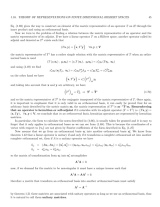
![1.14. THEORY OF REPRESENTATIONS IN FINITE-DIMENSIONAL VECTOR SPACES 39
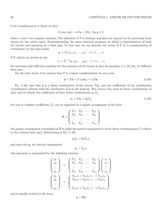
the last equality appears in matrix notation where T is the matrix representative of the linear operator T in the
ordered basis ui. Similarly, x and y are the coordinate representatives of the intrinsic vectors in the same ordered
basis. Eq. (1.49) shows clearly how to construct the matrix T, i.e. applying the operator to each vector in the
basis, and writing the new vectors as linear combinations of the basis. The coefficient of the i − th new vector
associated to the j − th element of the basis gives the element Tji in the associated matrix. Observe that for a
matrix representative to be possible, the linearity was fundamental in the procedure.
On the other hand, since we are looking for an isomorphism among linear transformations on V and the set
of matrices (as an algebra), we should define linear operations and product of matrices in such a way that these
operations are preserved in the algebra of linear transformations. In other words, if we denote by [T] the matrix
representative of T in a given ordered basis we should find operations with matrices such that
[T1 + T2] = [T1] + [T2] ; [αT] = α [T] ; [T1T2] = [T1] [T2]
we examine first the product by a scalar, according to the definition (1.7) we have
(αT) (ui) = α (Tui) = α (ujTji) = uj (αTji) ⇒
(αT) (ui) = uj (αTji) ⇒ (uj) (αT)ji = uj (αTji)
using linear independence we obtain the algorithm for scalar multiplication
(αT)ji = αTji
Now for the sum we use the definition 1.6
(T + U) uj = Tuj + Uuj = uiTij + uiUij = ui (Tij + Uij) ⇒
(T + U) uj = ui (Tij + Uij) ⇒ ui (T + U)ij = ui (Tij + Uij)
and along with linear independence it leads to
(T + U)ij = (Tij + Uij)
Moreover, for multiplication (composition) we use definition 1.9
(TU) ui = T (Uui) = T (ujUji) = UjiT (uj) = Uji (Tuj) = Uji (ukTkj) ⇒
(TU) ui = (TkjUji) uk ⇒ uk (TU)ki = uk (TkjUji)
linear independence gives
(TU)ki = TkjUji (1.50)
It can be easily shown that the matrix representations of the operators 0 and I are unique and equal in any
basis, they correspond to [0]ij = 0 and [I]ij = δij.
Finally, we can check from Eq. (1.49) that the mapping T → [T] is one-to-one and onto. It completes the proof
of the isomorphism between the set of linear transformations and the set of matrices as algebras.
On the other hand, owing to the one-to-one correspondence T ↔ [T] and the preservation of all operations, we
see that non-singular linear transformations (i.e. invertible linear transformations) should correspond to invertible
matrices. We denote
T−1
the matrix representative of T−1, and our goal is to establish the algorithm for this
inverse matrix, the definition of the inverse of the linear transformation is
TT−1
= T−1
T = I
since the representation of the identity is always [I]ij = δij, the corresponding matrix representation of this
equation is
[T]ik
T−1
kj
=
T−1
ik
[T]kj = δij (1.51)
this equation can be considered as the definition of the inverse of a matrix if it exists. A natural definition is then](https://image.slidesharecdn.com/cuantica-220626164623-64979fb3/85/cuantica-pdf-39-320.jpg)
![40 CAPÍTULO 1. LINEAR OR VECTOR SPACES
Definition 1.26 A matrix which does not admit an inverse is called a singular matrix. Otherwise, we call it a
non-singular matrix.
Since T−1 is unique, the corresponding matrix is also unique, so the inverse of a matrix is unique when it exists.
A necessary and sufficient condition for a matrix to have an inverse is that its determinant must be non-zero.
The algebra of matrices of dimension n × n is called the total matrix algebra An, the preceding discussion can
be summarized in the following
Theorem 1.51 if B = {u1, .., un} is an ordered basis of a vector space V of dimension n, the mapping T → [T]
which assigns to every linear transformation on V its matrix relative to B, is an isomorphism of the algebra of
the set of all linear transformations on V onto the total matrix algebra An.
Theorem 1.52 if B = {u1, .., un} is an ordered basis of a vector space V of dimension n, and T a linear
transformation whose matrix relative to B is [aij]. Then T is non-singular ⇔ [aij] is non-singular and in this case
[aij]−1
=
T−1
.
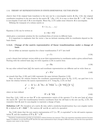
1.14.2. Change of coordinates of vectors under a change of basis
We have already seen that any vector space has an infinite number of bases. Notwithstanding, once a given
basis is obtained, any other one can be found by a linear transformation of the original basis.
Let {uj} be our “original” ordered basis and
n
u′
j
o
any other ordered basis. Each u′
i is a linear combination
of the original basis
u′
i = aijuj i = 1, . . . , n (1.52)
linear independence of {ui} ensures the uniqueness of the coefficients aij. The natural question is whether we
require any condition on the matrix representation aij in Eq. (1.52) to ensure that the set
n
u′
j
o
be linearly inde-
pendent. If we remember that there is a one-to-one correspondence between matrices and linear transformations
we see that aij must correspond to a (unique) linear transformation A. In this notation Eq. (1.52) becomes
u′
i = Auj (1.53)
now appealing to theorem 1.9 we see that
n
u′
j
o
is a basis if and only if A is non-singular, but A is non-singular
if and only if [A]ij = aij is a non-singular matrix. Thus Eq. (1.53) can be written in matrix notation as
u′
= Au (1.54)
the new set {u′
i} is a basis if and only if the matrix A is non-singular. Any vector x can be written in both bases
x = xiui = x′
iu′
i = x′
iaijuj = x′
jajiui (1.55)
and owing to the linear independence of ui
xi = x′
jaji = ãijx′
j ; ãij ≡ aji
where ãij ≡ aji indicates the transpose of the matrix A. In matrix form we have
u′
= Au , x = Ãx
′
(1.56)
and using Eq. (1.56) we get
x′
= Ã−1
x (1.57)](https://image.slidesharecdn.com/cuantica-220626164623-64979fb3/85/cuantica-pdf-40-320.jpg)
![44 CAPÍTULO 1. LINEAR OR VECTOR SPACES
Gram-Schmidt process for orthonormalization of linearly independent sets
From the previous discussion, it is very clear that complete orthonormal sets posses many advantages with
respect to other sets of linearly independent vectors. It leads us to study the possibility of finding an orthonormal set
from a given set of linearly independent vectors in a Hilbert space. The so-called Gram-Schmidt orthonormalization
process starts from an arbitrary set of independent vectors {x1, x2, .., xn, ...} on H and exhibits a recipe to construct
a corresponding orthonormal set {u1, u2, .., un, ...} with the property that for each n the vector subspace spanned
by {u1, u2, .., un} is the same as the one spanned by {x1, x2, .., xn}.
The gist of the procedure is based on Eqs. (1.24, 1.64). We start by normalizing the vector x1
u1 =
x1
kx1k
now we substract from x2 its component along u1 to obtain x2 − (u1, x2) u1 and normalized it
u2 =
x2 − (u1, x2) u1
kx2 − (u1, x2) u1k
it should be emphasized that x2 is not a scalar multiple of x1 so that the denominator above is non-zero. It is
clear that u2 is a linear combination of x1, x2 and that x2 is a linear combination of u1, u2. Therefore, {u1, u2}
spans the same subspace as {x1, x2}. The next step is to substract from x3 its components in the directions u1
and u2 to get a vector orthogonal to u1 and u2 according with Eq. (1.24). Then we normalize the result and find
u3 =
x3 − (u1, x3) u1 − (u2, x3) u2
kx3 − (u1, x3) u1 − (u2, x3) u2k
once again {u1, u2, u3} spans the same subspace as {x1, x2, x3}. Continuing this way we clearly obtain an ortho-
normal set {u1, u2, .., un, ...} with the stated properties.
Many important orthonormal sets arise from sequences of simple functions over which we apply the Gram-
Schmidt process
In the space L2 of square integrable functions associated with the interval [−1, 1], the functions xn (n =
0, 1, 2, ..) are linearly independent. Applying the Gram Schmidt procedure to this set we obtain the orthonormal
set of the Legendre Polynomials.
In the space L2 of square integrable functions associated with the entire real line, the functions xne−x2/2
(n = 0, 1, 2, ..) are linearly independent. Applying the Gram Schmidt procedure to this set we obtain the normalized
Hermite functions.
In the space L2 associated with the interval [0, +∞), the functions xne−x (n = 0, 1, 2, ..) are linearly indepen-
dent. Orthonormalizing it we obtain the normalized Laguerre functions.
Each of these orthonormal sets described above can be shown to be complete in their corresponding Hilbert
spaces.
1.16.1. Linear operators in finite dimensional Hilbert spaces
First of all let us see how to construct the matrix representation of a linear operator by making profit of the
inner product. Eq. (1.49) shows us how to construct the matrix representation of T in a given basis by applying
the operator to each element ui of such a basis
Tui = ujTji ⇒ (uk, Tui) = (uk, ujTji)
⇒ (uk, Tui) = Tjimkj
if the basis is orthonormal then mkj = δkj and
Tki = (uk, Tui) (1.69)](https://image.slidesharecdn.com/cuantica-220626164623-64979fb3/85/cuantica-pdf-44-320.jpg)
![(1.75)
so that if we multiply an n × n matrix by a scalar, the determinant is
|αA| = αn
|A| (1.76)
in particular
|−A| = (−1)n
|A| (1.77)
another important property is the trace of the matrix defined as the sum of its diagonal elements
TrA = aii (1.78)
we emphasize the sum over repeated indices. We prove that
Tr [AB] = Tr [BA] (1.79)
in this way
Tr [AB] = (AB)ii = aikbki = bkiaik = (BA)kk = Tr [BA]
it is important to see that the trace is cyclic invariant, i.e.
Tr
h
A(1)
A(2)
. . . A(n−2)
A(n−1)
A(n)
i
= Tr
h
A(n)
A(1)
A(2)
. . . A(n−2)
A(n−1)
i
= Tr
h
A(n−1)
A(n)
A(1)
A(2)
. . . A(n−2)
i
(1.80)](https://image.slidesharecdn.com/cuantica-220626164623-64979fb3/85/cuantica-pdf-100-320.jpg)

![48 CAPÍTULO 1. LINEAR OR VECTOR SPACES
In particular, the product of a column vector (m × 1 matrix) with a m × m matrix in the form xA cannot be
defined. Nevertheless, the product of the transpose of the vector (row vector) and the matrix A in the form e
xA
can be defined. In a similar fashion, the product Ae
x cannot be defined but Ax can. From these considerations
the quantities Ax and e
xA correspond to a new column vector and a new row vector respectively.
From the dimensions of the rectangular matrices we see that
Am×n ⇒ e
An×m and Bn×d ⇒ e
Bd×n
and the product AB is defined. However, their transposes can only be multiplied in the opposite order, i.e. in the
order e
B e
A. Indeed, it is easy to prove that, as in the case of square matrices, the transpose of a product is the
product of the transpose of each matrix in the product, but with the product in the opposite order. Applying this
property it can be seen that
]
(Ax) = e
x e
A ; ]
(e
xA) = e
Ax
where we have taken into account that the transpose of the transpose is the original matrix.
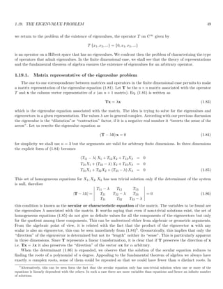
1.19. The eigenvalue problem
If T is a linear transformation on a vector space of finite dimension n, the simplest thing that the linear
transformation can do to a vector is to produce a “dilatation” or “contraction” on it, eventually changing the
“sense” of the “arrow” but keeping its “direction”. In algebraic words, certain vectors can be transformed by
T into a scalar multiple of itself. If x is a vector in H this operation is given by
Tx = λx (1.81)
a non-zero vector x such that Eq. (1.81) holds, is called an eigenvector of T, and the corresponding scalar λ is
called an eigenvalue of T. Each eigenvalue has one or more eigenvectors associated with it and to each eigenvector
corresponds a unique eigenvalue.
Let us assume for a moment that the set of eigenvalues for a given T is non-empty. For a given λ consider the
set M of all its eigenvectors together with the vector 0 (which is not an eigenvector), we denote this vectors as
x
(λ)
i . M is a linear subspace of H, we see it by taking an arbitrary linear combination of vectors in M
T
αix
(λ)
i
= αiT
x
(λ)
i
= αiλx
(λ)
i = λ
αix
(λ)
i
⇒
T
αix
(λ)
i
= λ
αix
(λ)
i
such that a linear combination is also an eigenvector with the same eigenvalue. Indeed, for Hilbert spaces it can
be shown that M is a closed vector subspace of H. As any vector space, M has many basis and if H is finite
dimensional, complete orthonormal sets are basis. The dimension of M is thus the maximum number of linearly
independent eigenvectors associated with λ. M is called the vector eigenspace generated by the eigenvalue λ. This
discussion induces the following
Definition 1.29 A given eigenvalue λ in Eq. (1.81) is called n−fold degenerate if n is the dimension of the
eigenspace M of H generated by λ. In other words, n is the maximum number of linearly independent eigenvectors
of λ. If n = 1 we say that λ is non-degenerate.
Even for non-degenerate eigenvalues we always have an infinite number of eigenvectors, for if x(λ) is an eigen-
vector, then αx(λ) is also an eigenvector for any scalar α. Eq. (1.81) can be written equivalently as
(T − λI) x = 0 (1.82)](https://image.slidesharecdn.com/cuantica-220626164623-64979fb3/85/cuantica-pdf-118-320.jpg)
![1.23. COMPLETE SETS OF COMMUTING OBSERVABLES (C.S.C.O.) 59
thus the matrix representation of A(p) is λpI for any orthonormal set complete in Mp (not neccesarily the original).
Now let us see the matrix representative of the restriction B(p) of B on Mp, writing this representation in our
original orthonormal set
B
(p)
ij = ui
p, Buj
p
since B is a self-adjoint operator this matrix is self-adjoint, and according to theorem 1.65 they can always be
diagonalized by a unitary transformation, which in turn means that there exists an orthonormal set
vi
p
in Mp
for which the matrix representative of B(p) is diagonal, hence
B
(p)
ij = vi
p, Bvj
p
= B
(p)
i δij
which means that the new orthonormal set complete in Mp consists of eigenvectors of B
Bvi
p = B
(p)
i vi
p
and since Mp contains only eigenvectors of A, it is clear that
vi
p
is an orthonormal set complete in Mp that
are common eigenvectors of A and B. Proceeding in this way with all eigensubspaces of A with more than one
dimension, we obtain a complete orthonormal set in H in which the elements of the set are common eigenvectors
of A and B.
It is important to emphasize that for a given Mp the orthonormal set chosen a priori does not in general consist
of eigenvectors of B, but it is always possible to obtain another orthonormal set that are eigenvectors of B and
by definition they are also eigenvectors of A.
Now let us prove that if A and B are observables with a complete orthonormal set of common eigenvectors
then they commute. Let us denote the complete orthonormal set of common eigenvectors as ui
n,p then
ABui
n,p = bpAui
n,p = anbpui
n,p
BAui
n,p = anBui
n,p = anbpui
n,p
therefore
[A, B] ui
n,p = 0
since ui
n,p form a complete orthonormal set, then [A, B] = 0.
It is also very simple to show that if A and B are commuting observables with eigenvalues an and bp and with
common eigenvectors ui
n,p then
C = A + B
is also an observable with eigenvectors ui
n,p and eigenvalues cn,p = an + bp.
1.23. Complete sets of commuting observables (C.S.C.O.)
Consider an observable A and a complete orthonormal set
ui
n
of the Hilbert space that consists of eigenvectors
of A. If none of the eigenvalues of A are degenerate then the eigenvalues determine the eigenvectors in a unique
way (within multiplicative constant factors). All the eigensubspaces Mi are one-dimensional and the complete
orthonormal set is simply denoted by {un}. This means that there is only one complete orthonormal set (except
for multiplicative phase factors) associated with the eigenvectors of the observable A. We say that A constitutes
by itself a C.S.C.O.
On the other hand, if some eigenvalues of A are degenerate, specifying an is not enough to determine a
complete orthonormal set for H because any orthonormal set in the eigensubspace Mn can be part of such a
complete orthonormal set. Thus the complete orthonormal set determined by the eigenvectors of A is not unique
and it is not a C.S.C.O.](https://image.slidesharecdn.com/cuantica-220626164623-64979fb3/85/cuantica-pdf-141-320.jpg)
![1.26. DISCRETE ORTHONORMAL BASIS 63
let us mention some important linear oprators on functions ψ (r) ∈ ̥.
The parity opeartor defined as
Πψ (x, y, z) = ψ (−x, −y, −z)
the product operator X defined as
Xψ (x, y, z) = xψ (x, y, z)
and the differentiation operator with respect to x denoted as Dx
Dxψ (x, y, z) =
∂ψ (x, y, z)
∂x
it is important to notice that the operators X and Dx acting on a function ψ (r) ∈ ̥, can transform it into a
function that is not square integrable. Thus it is not an operator of ̥ into ̥ nor onto ̥. However, the non-physical
states obtained are frequently useful for practical calculations.
The commutator of the product and differentiation operator is of central importance in quantum mechanics
[X, Dx] ψ (r) =
x
∂
∂x
−
∂
∂x
x
ψ (r) = x
∂
∂x
ψ (r) −
∂
∂x
[xψ (r)]
= x
∂
∂x
ψ (r) − x
∂
∂x
ψ (r) − ψ (r)
[X, Dx] ψ (r) = −ψ (r) ∀ψ (r) ∈ ̥
therefore
[X, Dx] = −I (1.105)
1.26. Discrete orthonormal basis
The Hilbert space L2 (and thus ̥) has a countable infinite dimension, so that any authentic basis of ̥ must
be infinite but discrete. A discrete orthonormal basis {ui (r)} with ui (r) ∈ ̥ should follows the rules given in
section 1.9.1. Thus orthonormality is characterized by
(ui, uj) =
Z
d3
r u∗
i (r) uj (r) = δij
the expansion of any wave function (vector) of this space is given by the Fourier expansion described by Eq. (1.27)
ψ (r) =
X
i
ciui (r) ; ci = (ui, ψ) =
Z
d3
r u∗
i (r) ψ (r) (1.106)
using the terminology for finite dimensional spaces we call the series a linear combination and ci are the components
or coordinates, which correspond to the Fourier coefficients. Such coordinates provide the representation of ψ (r)
in the basis {ui (r)}. It is very important to emphasize that the expansion of a given ψ (r) must be unique for
{ui} to be a basis, in this case this is guranteen by the form of the Fourier coefficients.
Now if the Fourier expansion of two wave functions are
ϕ (r) =
X
j
bjuj (r) ; ψ (r) =
X
i
ciui (r)
The scalar product and the norm can be expressed in terms of the components or coordinates of the vectors
according with Eqs. (1.65, 1.66)
(ϕ, ψ) =
X
i
b∗
i ci ; (ψ, ψ) =
X
i
|ci|2
(1.107)
and the matrix representation of an operator T in a given orthonormal basis {ui} is obtained from Eq. (1.69)
Tij ≡ (ui, Tuj)](https://image.slidesharecdn.com/cuantica-220626164623-64979fb3/85/cuantica-pdf-145-320.jpg)
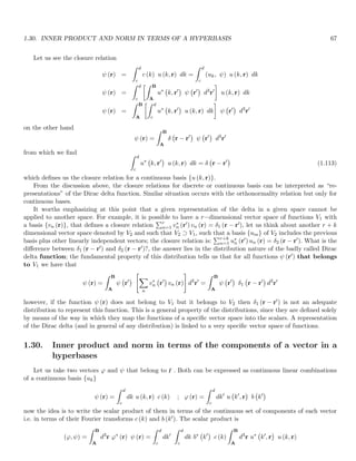
![64 CAPÍTULO 1. LINEAR OR VECTOR SPACES
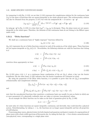
1.26.1. Función delta de Dirac
Como veremos a continuación la función delta de Dirac es un excelente instrumento para expresar el hecho
de que un conjunto ortonormal dado sea completo. También es útil para convertir densidades puntuales, lineales
y superficiales, en densidades volumétricas equivalentes. Es importante enfatizar que la función delta de Dirac
mas que una función es una distribución. En el lenguaje del análisis funcional, es una uno-forma que actúa en
espacios vectoriales de funciones, asignándole a cada elemento del espacio, un número real de la siguiente forma:
Sea V el espacio vectorial de las funciones definidas en el dominio (b, c) con ciertas propiedades de continuidad,
derivabilidad, integrabilidad, etc. La distribución delta de Dirac es un mapeo que asigna a cada elemento f (x) de
V un número real con el siguiente algoritmo8
Z c
b
f (x) δ (x − a) dx =
f (a) si a ∈ (b, c)
0 si a /
∈ [b, c]
mencionaremos incidentalmente que con esta distribución es posible escribir una densidad de carga (o masa)
puntual (ubicada en r0) como una densidad volumétrica equivalente
ρ (r) = qδ r′
− r0
(1.108)
esta densidad reproduce adecuadamente tanto la carga total como el potencial y el campo que genera, una vez
que se hagan las integrales apropiadas.
Hay varias sucesiones de distribuciones que convergen a la función Delta de Dirac, una de las mas utilizadas
es la sucesión definida por
fn (x − a) =
n
√
π
e−n2(x−a)2
(1.109)
se puede demostrar que al tomar el lı́mite cuando n → ∞ se reproduce la definición y todas las propiedades básicas
de la distribución delta de Dirac. Nótese que todas las distribuciones gaussianas contenidas en esta sucesión tienen
área unidad y están centradas en a. De otra parte, a medida que aumenta n las campanas gaussianas se vuelven
más agudas y más altas a fin de conservar el área, para valores n suficientemente altos, el área se concentra en
una vecindad cada vez más pequeña alrededor de a. En el lı́mite cuando n → ∞, toda el área se concentra en un
intervalo arbitrariamente pequeño alrededor de a.
Algunas propiedades básicas son las siguientes:
1.
R ∞
−∞ δ (x − a) dx = 1
2.
R ∞
−∞ f (x) ∇δ (r − r0) dV = − ∇f|r=r0
3. δ (ax) = 1
|a| δ (x)
4. δ (r − r0) = δ (r0 − r)
5. xδ (x) = 0
6. δ x2 − e2
= 1
2|e| [δ (x + e) + δ (x − e)]
Vale enfatizar que debido a su naturaleza de distribución, la función delta de Dirac no tiene sentido por sı́ sola,
sino únicamente dentro de una integral. Por ejemplo cuando decimos que δ (ax) = 1
|a| δ (x), no estamos hablando
8
Es usual definir la “función” delta de Dirac como δ (r) =
∞ si r = 0
0 si r 6= 0
y
R
δ (x) dx = 1. Esta definición se basa en una
concepción errónea de la distribución delta de Dirac como una función. A pesar de ello, hablaremos de ahora en adelante de la función
delta de Dirac para estar acorde con la literatura.](https://image.slidesharecdn.com/cuantica-220626164623-64979fb3/85/cuantica-pdf-146-320.jpg)
![66 CAPÍTULO 1. LINEAR OR VECTOR SPACES
1.28. Introduction of hyperbases
In the case of discrete basis each element ui (r) is square integrable and thus belong to L2 and in general to ̥
as well. As explained before, it is sometimes convenient to use some hyperbases in which the elements of the basis
do not belong to either L2 or ̥, but in terms of which a function in ̥ can be expanded, the hyperbasis {u (k, r)}
will have in general a continuous cardinality with k denoting the continuous index that labels each vector in the
hyperbasis. According to our previous discussions the Fourier expansions made with this hyperbasis are not series
but integrals, these integrals will be called continuous linear combinations.
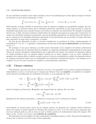
1.29. Closure relation with hyperbases
In the hyperbasis {u (k, r)}, k is a continuous index defined in a given interval [c, d]. Such an index makes
the role of the index n in discrete bases. We shall see that a consistent way of expressing orthonormality for this
continuous basis is9
(uk, uk′ ) =
Z B
A
u∗
(k, r) u k′
, r
d3
r = δ k − k′
(1.111)
we show it by reproducing the results obtained with discrete bases. Expanding an arbitrary function ψ (r) of our
Hilbert space as a continuous linear combination of the basis gives
ψ (r) =
Z d
c
c (k) u (k, r) dk
then we have
(uk′ , ψ) =
uk′ ,
Z d
c
c (k) u (k, r) dk
=
Z d
c
c (k) (uk′ , uk) dk
=
Z d
c
c (k) δ k − k′
dk = c k′
from which the fourier coefficients of the continuous expansion are evaluated as
c k′
= (uk′ , ψ) (1.112)
when the Fourier coefficients are associated with continuous linear combinations (integrals) they are usually called
Fourier transforms. In this case, a vector is represented as a continuous set of coordinates or components, where
the components or coordinates are precisely the Fourier transforms.
Therefore, in terms of the inner product, the calculation of the Fourier coefficients in a continuous basis
(Fourier transforms) given by Eq. (1.112) coincides with the calculation of them with discrete bases Eq. (1.106).
Eq. (1.112) in turn guarantees that the expansion for a given ordered continuous bases is unique10. Those facts
in turn depends strongly on our definition of orthonormality in the continuous regime Eq. (1.111) showing the
consistency of such a definition. After all, we should remember that hyperbases are constructed as useful tools
and not as physical states, in that sense we should not expect a “truly orthonormality relation” between them11.
9
From now on we shall say continuous bases, on the understanding that they are indeed hyperbases.
10
Remember that for a given set of vectors to constitute a basis, it is important not only to be able to expand any vector with
the elements of the set, it is also necessary for the expansion of each vector to be unique. In normal basis (not hyperbasis) this is
guaranteed by the linear independence, in our continuous set it is guranteed by our definition of orthonormality in such a set.
11
It is clear for example that with r = r′
the “orthonormality” relation diverge, so it is not a normalization in the mathematical
sense.](https://image.slidesharecdn.com/cuantica-220626164623-64979fb3/85/cuantica-pdf-148-320.jpg)
![70 CAPÍTULO 1. LINEAR OR VECTOR SPACES
1.32. Tensor products of vector spaces, definition and properties
Let V1 and V2 be two vector spaces of dimension n1 and n2. Vectors and operators on each of them will be
denoted by labels (1) and (2) respectively.
Definition 1.34 The vector space V is called the tensor product of V1 and V2
V ≡ V1 ⊗ V2
if there is associated with each pair of vectors x (1) ∈ V1 and y (2) ∈ V2 a vector in V denoted by x (1) ⊗ y (2) and
called the tensor product of x (1) and y (2), and in which this correspondence satisfies the following conditions:
(a) It is linear with respect to multiplication by a scalar
[αx (1)] ⊗ y (2) = α [x (1) ⊗ y (2)] ; x (1) ⊗ [βy (2)] = β [x (1) ⊗ y (2)] (1.123)
(b) It is distributive with respect to addition
x (1) + x′
(1)
⊗ y (2) = x (1) ⊗ y (2) + x′
(1) ⊗ y (2)
x (1) ⊗
y (2) + y′
(2)
= x (1) ⊗ y (2) + x (1) ⊗ y′
(2) (1.124)
(c) When a basis is chosen in each space, say {ui (1)} in V1 and {vj (2)} in V2, the set of vectors ui (1) ⊗ vj (2)
constitutes a basis in V . If n1 and n2 are finite, the dimension of the tensor product space V is n1n2.
An arbitrary couple of vectors x (1), y (2) can be written in terms of the bases {ui (1)} and {vj (2)} respectively,
in the form
x (1) =
X
i
aiui (1) ; y (2) =
X
j
bjvj (2)
Using Eqs. (1.123, 1.124) we see that the expansion of the tensor product is given by
x (1) ⊗ y (2) =
X
i
X
j
aibjui (1) ⊗ vj (2)
so that the components of the tensor product of two vectors are the products of the components of the two vectors of
the product. It is clear that the tensor product is commutative i.e. V1 ⊗V2 = V2 ⊗V1 and x (1)⊗y (2) = y (2)⊗x (1)
On the other hand, it is important to emphasize that there exist in V some vectors that cannot be written
as tensor products of a vector in V1 with a vector in V2. Nevertheless, since {ui (1) ⊗ vj (2)} is a basis in V any
vector in V can be expanded in it
ψ =
X
i
X
j
cijui (1) ⊗ vj (2) (1.125)
in other words, given a set of n1n2 coefficients of the form cij it is not always possible to write them as products
of the form aibj of n1 numbers ai and n2 numbers bj, we cannot find always a couple of vectors in V1 and V2 such
that ψ = x (1) ⊗ y (2).
1.32.1. Scalar products in tensor product spaces
If there are inner products defined in the spaces V1 and V2 we can define an inner product in the tensor product
space V . For a couple of vectors in V of the form x (1) ⊗ y (2) the inner product can be written as
x′
(1) ⊗ y′
(2) , x (1) ⊗ y (2)
= x′
(1) , x (1)
(1)
y′
(2) , y (2)
(2)](https://image.slidesharecdn.com/cuantica-220626164623-64979fb3/85/cuantica-pdf-152-320.jpg)
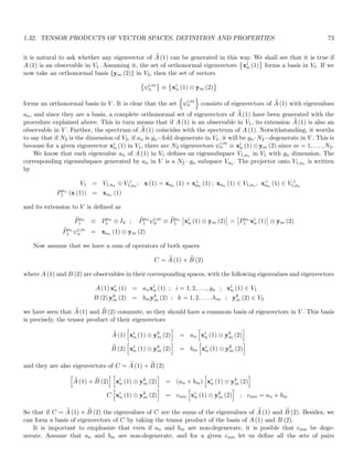
![1.32. TENSOR PRODUCTS OF VECTOR SPACES, DEFINITION AND PROPERTIES 71
where the symbols (, )(1) and (, )(2) denote the inner product of each of the spaces of the product. From this, we can
see that if the bases {ui (1)} and {vj (2)} are orthonormal in V1 and V2 respectively, then the basis {ui (1) ⊗ vj (2)}
also is
(ui (1) ⊗ vj (2) , uk (1) ⊗ vm (2)) = (ui (1) , uk (1))(1) (vj (2) , vm (2))(2) = δikδjm
Now, for an arbitrary vector in V , we use the expansion (1.125) and the basic properties of the inner product
(ψ, φ) =
X
i
X
j
cijui (1) ⊗ vj (2) ,
X
k
X
m
bkmuk (1) ⊗ vm (2)
=
X
i,j
c∗
ij
X
k,m
bkm (ui (1) ⊗ vj (2) , uk (1) ⊗ vm (2)) =
X
i,j
c∗
ij
X
k,m
bkmδikδjm
(ψ, φ) =
X
i,j
c∗
ijbij
it is easy to show that with these definitions the new product accomplishes the axioms of an inner product.
1.32.2. Tensor product of operators
Consider a linear transformation A (1) defined in V1, we associate with it a linear operator e
A (1) acting on V
as follows: when e
A (1) is applied to a tensor of the type x (1) ⊗ y (2) we define
e
A (1) [x (1) ⊗ y (2)] = [A (1) x (1)] ⊗ y (2)
when the operator is applied to an arbitrary vector in V , this definition is easily extended because of the linearity
of the transformation
e
A (1) ψ = e
A (1)
X
i
X
j
cijui (1) ⊗ vj (2) =
X
i
X
j
cij
e
A (1) [ui (1) ⊗ vj (2)]
e
A (1) ψ =
X
i
X
j
cij [A (1) ui (1)] ⊗ vj (2) (1.126)
the extension e
B (2) of a linear transformation in V2 is obtained in a similar way
e
B (2) ψ =
X
i
X
j
cijui (1) ⊗ [B (2) vj (2)]
finally, if we consider two operators A (1) , B (2) defined in V1 and V2 respectively, we can define their tensor
product A (1) ⊗ B (2) as
[A (1) ⊗ B (2)] ψ =
X
i
X
j
cij [A (1) ui (1)] ⊗ [B (2) vj (2)] (1.127)
it is easy to show that A (1) ⊗ B (2) is also a linear operator. From Eqs. (1.126, 1.127) we can realize that the
extension of the operator A (1) on V1 to an operator e
A (1) on V can be seen as the tensor product of A (1) with
the identity operator I (2) on V2. A similar situation occurs with the extension e
B (2)
e
A (1) = A (1) ⊗ I (2) ; e
B (2) = I (1) ⊗ B (2) (1.128)
Now let us put the operators A (1)⊗B (2) and e
A (1) e
B (2) to act on an arbitrary element of a basis {ui (1) ⊗ vj (2)}
of V
[A (1) ⊗ B (2)] ui (1) ⊗ vj (2) = [A (1) ui (1)] ⊗ [B (2) vj (2)]
h
e
A (1) e
B (2)
i
ui (1) ⊗ vj (2) = e
A (1) {ui (1) ⊗ [B (2) vj (2)]} = [A (1) ui (1)] ⊗ [B (2) vj (2)]](https://image.slidesharecdn.com/cuantica-220626164623-64979fb3/85/cuantica-pdf-153-320.jpg)
![72 CAPÍTULO 1. LINEAR OR VECTOR SPACES
therefore, the tensor product A (1) ⊗ B (2) coincides with the ordinary product of two operators e
A (1) and e
B (2)
on V
A (1) ⊗ B (2) = e
A (1) e
B (2)
additionally, it can be shown that operators of the form e
A (1) and e
B (2) commute in V . To see it, we put their
products in both orders to act on an arbitrary vector of a basis {ui (1) ⊗ vj (2)} of V
h
e
A (1) e
B (2)
i
ui (1) ⊗ vj (2) = e
A (1) {ui (1) ⊗ [B (2) vj (2)]} = [A (1) ui (1)] ⊗ [B (2) vj (2)]
h
e
B (2) e
A (1)
i
ui (1) ⊗ vj (2) = e
B (2) {[A (1) ui (1)] ⊗ vj (2)} = [A (1) ui (1)] ⊗ [B (2) vj (2)]
therefore we have h
e
A (1) , e
B (2)
i
= 0 or A (1) ⊗ B (2) = B (2) ⊗ A (1)
an important special case of linear operators are the projectors, as any other linear operator, the projector in V is
the tensor product of the projectors in V1 and V2. Let M1 and N1 be the range and null space of a projector in
V1 and M2, N2 the range and null space of a projector in V2
V1 = M1 ⊕ N1 ; x (1) = xM (1) + xN (1) ; xM (1) ∈ M1, xN (1) ∈ N1 ; P1 (x (1)) = xM (1)
V2 = M2 ⊕ N2 ; y (2) = yM (2) + yN (2) ; yM (2) ∈ M2, yN (2) ∈ N2 ; P2 (y (2)) = yM (2)
(P1 ⊗ P2) (x (1) ⊗ y (2)) = [P1x (1)] ⊗ [P2y (2)] = xM (1) ⊗ yM (2)
for an arbitrary vector we have
(P1 ⊗ P2) ψ = (P1 ⊗ P2)
X
i
X
j
cijui (1) ⊗ vj (2) =
X
i
X
j
cij [P1ui (1)] ⊗ [P2vj (2)]
(P1 ⊗ P2) ψ =
X
i
X
j
cijui,M (1) ⊗ vj,M (2)
finally, as in the case of vectors, there exists some operators on V that cannot be written as tensor products of
the form A (1) ⊗ B (2).
1.32.3. The eigenvalue problem in tensor product spaces
Let us assume that we have solved the eigenvalue problem for an operator A (1) of V1. We want to seek for
information concerning the eigenvalue problem for the extension of this operator to the tensor product space V .
For simplicity, we shall assume a discrete spectrum
A (1) xi
n (1) = anxi
n (1) ; i = 1, 2, . . . , gn ; xi
n (1) ∈ V1
where gn is the degeneration associated with an. We want to solve the eigenvalue problem for the extension of
this operator in V = V1 ⊗ V2
e
A (1) ψ = λψ ; ψ ∈ V1 ⊗ V2
from the definition of such an extension, we see that a vector of the form xi
n (1) ⊗ y (2) for any y (2) ∈ V2 is an
eigenvector of e
A (1) with eigenvalue an
e
A (1)
xi
n (1) ⊗ y (2)
=
A (1) xi
n (1)
⊗ y (2) = anxi
n (1) ⊗ y (2) ⇒
e
A (1)
xi
n (1) ⊗ y (2)
= an
xi
n (1) ⊗ y (2)](https://image.slidesharecdn.com/cuantica-220626164623-64979fb3/85/cuantica-pdf-154-320.jpg)
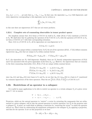
![74 CAPÍTULO 1. LINEAR OR VECTOR SPACES
{(nj, mj) : j = 1, . . . , q} such that anj + bmj = cnm. In that case, the eigenvalue cnm is q−fold degenerate, and
every eigenvector corresponding to this eigenvalue can be written as
q
X
j=1
cj
xnj (1) ⊗ ymj (2)
in this case there are eigenvectors of C that are not tensor products.
1.32.4. Complete sets of commuting observables in tensor product spaces
For simplicity assume that A (1) forms a C.S.C.O. by itself in V1, while {B (2) , C (2)} constitute a C.S.C.O.
in V2. We shall show that by gathering the operators of the C.S.C.O. in V1 with the operators of C.S.C.O. in V2,
we form a C.S.C.O. in V with their corresponding extensions.
Since A (1) is a C.S.C.O. in V1, all its eigenvalues are non-degenerate in V1
A (1) xn (1) = anx (1)
the ket x (1) is then unique within a constant factor. In V2 the set of two operators {B (2) , C (2)} defines commom
eigenvectors {ymp (2)} that are unique in V2 within constant factors
B (2) ymp (2) = bmymp (2) ; C (2) ymp (2) = cpymp (2)
In V , the eigenvalues are N2−fold degenerate. Similarly, there are N1 linearly independent eigenvectors of B (2)
and C (2) associated with two given eigenvalues of the form (bm, cp). However, the eigenvectors that are common
to the three commuting observables e
A (1) , e
B (2) , e
C (2) are unique within constant factors
e
A (1) [xn (1) ⊗ ymp (2)] = an [x (1) ⊗ ymp (2)]
e
B (2) [xn (1) ⊗ ymp (2)] = bm [x (1) ⊗ ymp (2)]
e
C (2) [xn (1) ⊗ ymp (2)] = cp [x (1) ⊗ ymp (2)]
since {xn (1)} and {ymp (2)} were bases in V1 and V2, we see that {xn (1) ⊗ ymp (2)} is a basis in V constituted
by commom eigenvectors of the three operators. Thus the set
n
e
A (1) , e
B (2) , e
C (2)
o
is a C.S.C.O. in V .
1.33. Restrictions of an operator to a subspace
It is useful in many applications to be able to restrict an operator to a certain subspace Vq of a given vector
space V . Let us assume
V = V1 ⊕ . . . ⊕ Vq ⊕ . . .
x = x1 + . . . + xq + . . . ; xi ∈ Vi
Projectors, which are the natural operators to “restrict” a vector by extracting the components that are ortho-
normal to a given subspace, will be also the natural operators to rectrict operators. Let Pq be the projector onto
a subspace Vq. A priori, we could think in defining a restriction by “restricting the vector” in which the operator
will act on. This is done by substracting all components orthogonal to the subspace Vq by applying a projection,
and then let the operator A act on this projection so we have
A = APq ⇒ Ax = APqx = Axq](https://image.slidesharecdn.com/cuantica-220626164623-64979fb3/85/cuantica-pdf-156-320.jpg)
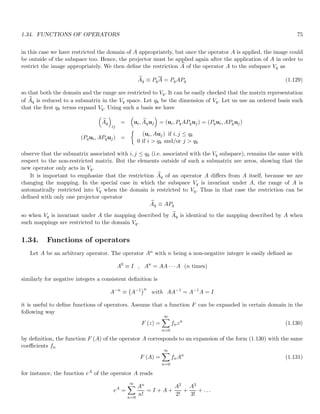
![76 CAPÍTULO 1. LINEAR OR VECTOR SPACES
the convergence of series of the type (1.131) depends on the eigenvalues of A and the radius of convergence of the
function (1.130). We shall not treat this topic in detail.
If F (z) is a real function the coefficients fn are real. On the other hand, if A is hermitian then F (A) also is,
as can be seen from (1.131). Owing to the analogy between real numbers and hermitian operators this relation is
quite expected. Now, assume that xi,k is an eigenvector of A with eigenvalue ai we then have
Axi,k = aixi,k ⇒ An
xi,k = an
i xi,k
and applying the eigenvector in Eq. (1.131) we find
F (A) xi,k =
∞
X
n=0
fnan
i xi,k = xi,k
∞
X
n=0
fnan
i
F (A) xi,k = F (ai) xi,k
so that if xi,k is an eigenvector of A with eigenvalue ai, then xi,k is also eigenvector of F (A) with eigenvalue
F (ai).
On the other hand, if the operator is diagonalizable (this is the case for observables), we can find a basis in
which the matrix representative of A is diagonal with the eigenvalues ai in the diagonal. In such a basis, the
operator F (A) has also a diagonal representation with elements F (ai) in the diagonal. For example let σz be an
operator that in certain basis has the matrix representation
σz =
1 0
0 −1
in the same basis we have
eσz
=
e1 0
0 e−1
=
e 0
0 1/e
if A and B do not commute, we have that in general the operators F (A) and F (B) do not commute either. For
instance
eA
eB
=
∞
X
n=0
An
n!
∞
X
m=0
Bm
m!
=
∞
X
n=0
∞
X
m=0
An
n!
Bm
m!
(1.132)
eB
eA
=
∞
X
m=0
Bm
m!
∞
X
n=0
An
n!
=
∞
X
m=0
∞
X
n=0
Bm
m!
An
n!
(1.133)
eA+B
=
∞
X
n=0
(A + B)n
n!
(1.134)
these three expressions are in general different from each other unless [A, B] = 0. We see by direct inspection
of Eqs. (1.132, 1.133, 1.134) that if A and B commute, then F (A) and F (B) also do. Notice that when A, B
commute they can be diagonalized simultaneously and so F (A) and F (B), which is another way to see that if
[A, B] = 0 then [F (A) , F (B)] = 0.
1.34.1. Some commutators involving functions of operators
Theorem 1.70 Suppose we have two operators A and B such that B commutes with their commutator, that is
[B, C] = 0 ; C ≡ [A, B] (1.135)
if F (B) is a function of the operator B then we have
[A, F (B)] = [A, B] F′
(B) (1.136)](https://image.slidesharecdn.com/cuantica-220626164623-64979fb3/85/cuantica-pdf-158-320.jpg)
![1.35. DIFFERENTIATION OF OPERATORS 77
where F′ (B) is the derivative of F (B) “with respect to B” defined as
F (B) =
∞
X
n=0
fnBn
⇒ F′
(B) ≡
∞
X
n=0
nfnBn−1
(1.137)
Proof: The commutator [A, F (B)] is given by
[A, F (B)] =
A,
∞
X
n=0
fnBn
#
=
∞
X
n=0
fn [A, Bn
] (1.138)
we show by induction that
[A, Bn
] = [A, B] nBn−1
(1.139)
for n = 0 we have Bn = I and both sides clearly vanish. Now let us assume that it works for n and show that it
is satisfied by n + 1. Applying Eq. (1.41), and taking into account Eqs. (1.139, 1.135) we have
A, Bn+1
= [A, BBn
] = [A, B] Bn
+ B [A, Bn
] = [A, B] BBn−1
+ B [A, B] nBn−1
= CBBn−1
+ BCnBn−1
= CBn
+ nCBBn−1
= C (n + 1) Bn
A, Bn+1
= [A, B] (n + 1) Bn
which shows the validity of Eq. (1.139). Replacing Eq. (1.139) in Eq. (1.138), we find
[A, F (B)] = [A, B]
∞
X
n=0
fnnBn−1
= [A, B] F′
(B)
Corollary 1.71 It is straightforward to show that if both operators commute with their commutator we see that
equations
[A, F (B)] = [A, B] F′
(B) ; [G (A) , B] = [A, B] G′
(B) (1.140)
are satisfied simultaneously. A very important case in Physics occurs when [A, B] = αI. In that case, we have
[A, B] = αI ⇒ [A, F (B)] = αF′
(B) ; [G (A) , B] = αG′
(B) (1.141)
1.35. Differentiation of operators
Let A (z) an operator that depends on the arbitrary variable z. We define the derivative of A (z) with respect
to z as
dA
dz
= lı́m
∆z→0
A (z + ∆z) − A (z)
∆z
(1.142)
provided that this limit exists. Operating A on an arbitrary vector x and using a basis {ui} independent of z, we
have
A (z) x = A (z) xiui = xiA (z) ui = xiujAji (z) (1.143)
since dA/dz is another operator, it makes sense to talk about its matrix representation
dA (z)
dz
x =
dA (z)
dz
xiui = xi
dA (z)
dz
ui = xiuj
dA (z)
dz
ji
(1.144)
Applying the derivative on both extremes of Eq. (1.143), and taking into account that the basis {ui} is independent
of z, we have
d
dz
A (z) x = xiuj
dAji (z)
dz
(1.145)](https://image.slidesharecdn.com/cuantica-220626164623-64979fb3/85/cuantica-pdf-159-320.jpg)
![78 CAPÍTULO 1. LINEAR OR VECTOR SPACES
comparing Eqs. (1.144, 1.145) we obtain
dA (z)
dz
ji
=
dAji (z)
dz
so the matrix representative of the derivative of A is obtained by taking the derivative of each of its elements12.
The differentiation rules are similar to the ones in ordinary calculus
d
dz
(F + G) =
dF
dz
+
dG
dz
;
d
dz
(FG) =
dF
dt
G + F
dG
dt
(1.146)
except that care must be taken with the order of appearance for the operators involved. Let us examine the second
of this equations, applying FG to an arbitrary vector x and using a basis {ui} we have
(FG) x = xiuj (FG)ji
taking the derivative on both sides we have
d (FG)
dz
ji
=
d
dz
(FG)ji =
d
dz
[FjkGki] =
d
dz
Fjk
Gki + Fjk
d
dz
Gki
=
dF
dz
jk
Gki + Fjk
dG
dz
ki
#
in matrix form we see that
d (FG)
dz
=
dF
dz
G + F
dG
dz
since there is a one-to-one isomorphism from the operators onto the matrices, we see that this relation is also valid
for the operators.
1.35.1. Some useful formulas
Applying the derivation rules we can develop some identities for functions of operators. Let us calculate the
derivative of the operator eAt. By definition we have
eAt
=
∞
X
n=0
(At)n
n!
differentiating the series term by term we have
d
dt
eAt
=
∞
X
n=0
ntn−1 An
n!
= 0 +
∞
X
n=1
ntn−1 An
n!
= A
∞
X
n=1
(At)n−1
(n − 1)!
d
dt
eAt
= A
∞
X
k=0
(At)k
k!
#
=
∞
X
k=0
(At)k
k!
#
A
where we have used the assignment k = n − 1. The series in the brackets is eAt once again, so we have
d
dt
eAt
= AeAt
= eAt
A (1.147)
12
Care must be taken to distinguish between the derivative in Eq. (1.137) and the derivative in Eq. (1.142). In Eq. (1.137) the
derivative is taken with respect to B as the “variable of derivation”. On the other hand, in Eq. (1.142) the variable to derive with, is
a parameter z from which our matrix depend on.](https://image.slidesharecdn.com/cuantica-220626164623-64979fb3/85/cuantica-pdf-160-320.jpg)
![1.36. STATE SPACE AND DIRAC NOTATION 79
in this case eAt and A commutes because only one operator is involved. Suppose that we want to differentiate
eAteBt. Applying Eqs. (1.146, 1.147) we have
d
dt
eAt
eBt
=
d eAt
dt
eBt
+ eAt d eBt
dt
= AeAt
eBt
+ eAt
BeBt
the operator A can pass over eAt if desired but not over eBt unless that A and B commute. Similarly, B can pass
over eBt but not over eAt.
However, even if a single operator appears we should be careful with the order sometimes. For instance, if A (t)
is an arbitrary function of time then
d
dt
eA(t)
6=
dA
dt
eA(t)
(1.148)
it could be checked that A (t) and dA (t) /dt must commute with each other for the equality to be valid.
Consider again two operators that commute with their commutator, we shall show that
[A, [A, B]] = [B, [A, B]] = 0 ⇒ eA
eB
= eA+B
e
1
2
[A,B]
(Glauber′
s formula) (1.149)
let define F (t) with t real as
F (t) ≡ eAt
eBt
;
dF (t)
dt
= AeAt
eBt
+ eAt
BeBt
= A eAt
eBt
+ eAt
Be−At
eAt
eBt
dF (t)
dt
=
A + eAt
Be−At
F (t) (1.150)
since A, B commute with their commutator, we can apply Eq. (1.140), so that
eAt
, B
= t [A, B] eAt
⇒ eAt
B = BeAt
+ t [A, B] eAt
⇒ eAt
Be−At
= B + t [A, B]
substituting this expression in Eq. (1.150) we get
dF (t)
dt
= {A + B + t [A, B]} F (t) (1.151)
by hypothesis, A+B commutes with [A, B], so that the differential equation (1.151) can be integrated as if A+B
and [A, B] were numbers
F (t) = F (0) e(A+B)t+ 1
2
[A,B]t2
setting t = 0 we see that F (0) = I, thus we obtain
F (t) = e(A+B)t+ 1
2
[A,B]t2
setting t = 1 and taking into account again that A + B commutes with [A, B], we obtain (1.149). It is necessary
to emphasize that this equation is valid only if A and B commutes with [A, B].
1.36. State space and Dirac notation
We have defined the space of Physical states as the one constituted by functions ψ (r) square-integrable
in a given volume. The space with these characteristics is denoted by L2, but since in general with add some
requirements to these functions, we actually work in a subspace ̥ ⊆ L2. On the other hand, we have seen that
several bases can be constructed to represent those functions. Therefore, the Physical system will be described
by either the functions ψ (r) or by the sete of its coordinates in a given representation. When the representation](https://image.slidesharecdn.com/cuantica-220626164623-64979fb3/85/cuantica-pdf-161-320.jpg)
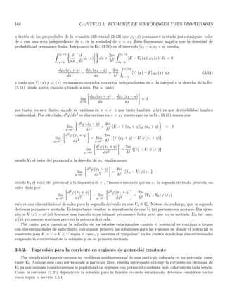
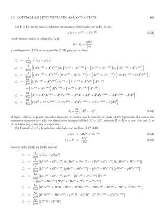
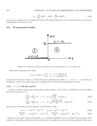
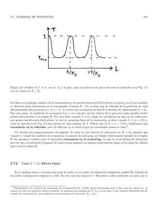
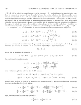
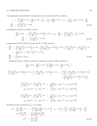
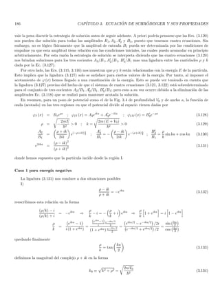
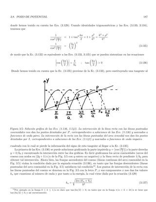
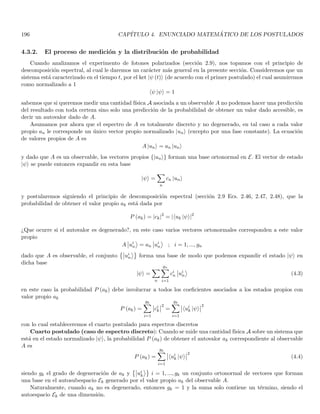
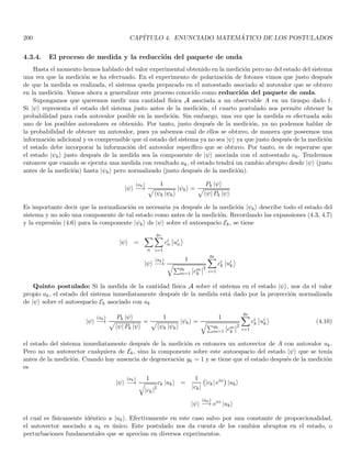
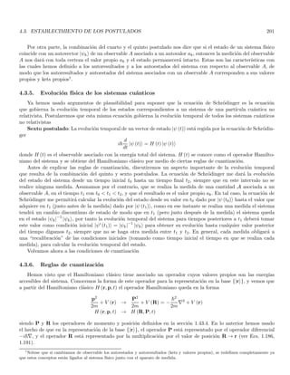
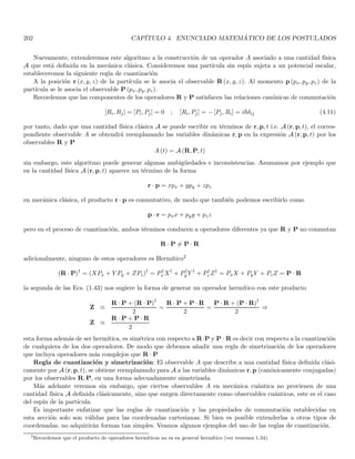
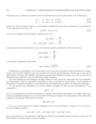
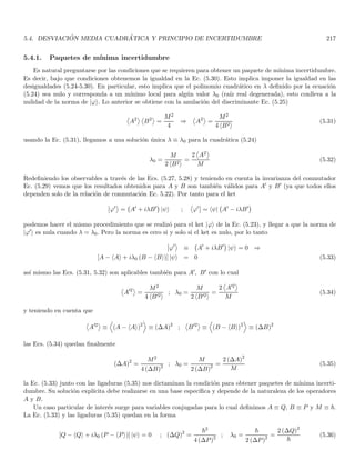
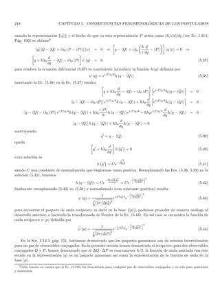
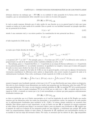
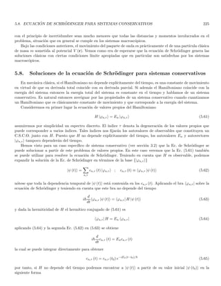
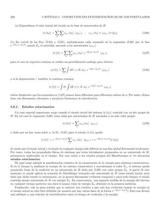
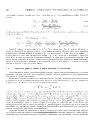


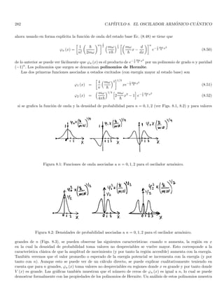
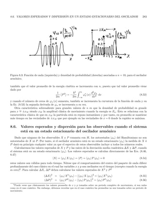
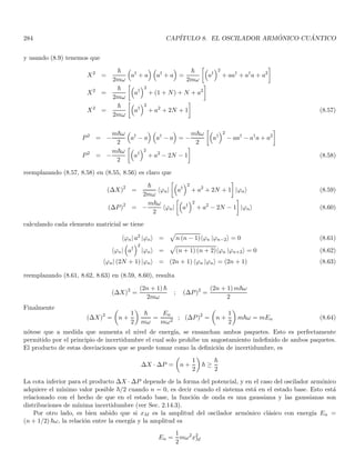
![1.39. HERMITIAN CONJUGATION 87
We shall now define a useful operation that we call hermitian conjugation. Our basic objects are kets, bras,
operators and scalars. In general words, hermitian conjugations are mappings induced by the existence of the dual
E∗ of our Hilbert space E.
A ket |ψi ∈ E is naturally mapped into a bra hψ| ∈ E∗.
A bra hψ| ∈ E∗ is naturally mapped into an element of the conjugate space of E∗, i.e on E∗∗. However, for
Hilbert spaces it can be shown that E∗∗ = E hence the bra is mapped into its corresponding ket16.
An operator A in ß(E) is mapped naturally into the conjugate vector A∗ in ß(E∗) but the inner product
structure permits in turn to define another operator A† in ß(E) from A∗ and from the practical point of view we
regard A∗ and A† as identical. Thus the hermitian conjugation in this case will be the mapping A → A†.
Now finally for scalars. Taking into account that for all practical uses scalars λ can be considered as operators
in ß(E) of the form λI we see that the natural hermitian conjugation gives λI → (λI)†
= λ∗. Therefore, the
natural conjugation operation is λ → λ∗.
We notice now that the hermitian conjugation reverses the order of the objects to which it is applied. We have
seen that (A |ψi)†
= hψ| A†, Eq. (1.165) shows that the order of a product of operators is reversed when we apply
the “adjointness” (or hermitian conjugation) on that product, when scalars are involved the place in which scalars
are located is irrelevant.
By the same token, let us see what is the conjugate of the non orthogonal projection defined in (1.159)
P = |ψi hϕ| ; P†
= (|ψi hϕ|)†
applying Eq. (1.163) we find
hχ| (|ψi hϕ|)†
|ηi = [hη| (|ψi hϕ|) |χi]∗
= hη| ψi∗
hϕ| χi∗
= hχ| ϕi hψ| ηi
hχ| (|ψi hϕ|)†
|ηi = hχ| (|ϕi hψ|) |ηi ; ∀ |ηi , |χi ∈ E
then we have
(|ψi hϕ|)†
= |ϕi hψ| (1.167)
once again, the hermitian conjugation converts each object in its hermitian conjugate and reverse the order of
such objects.
These observations permit to give a rule to obtain the hermitian conjugate of a mathematical object composed
by a juxtaposition of bras, kets, operators and scalars. The rule is (a) replace each object by its hermitian conjugate
|ψi → hψ| , hϕ| → |ϕi , A → A†
, λ → λ∗
and (b) reverse the order of the factors, taking into account that the position of the scalars are not relevant.
The hermitian conjugate of the objects defined in (1.166) are given by
[λ hϕ| B |ψi]†
= hψ| B†
|ϕi λ∗
= λ∗
hψ| B†
|ϕi = [λ hϕ| B |ψi]∗
[λ hψ| B |ϕi]†
= hϕ| B†
|ψi λ∗
= λ∗
hϕ| B†
|ψi = [λ hψ| B |ϕi]∗
[λ hψ| ϕiB]†
= B†
hϕ| ψiλ∗
= λ∗
hϕ| ψiB†
= (λ hψ| ϕi)∗
B†
[λ |ψi hϕ| B]†
= B†
|ϕi hψ| λ∗
= λ∗
B†
|ϕi hψ| = λ∗
B†
[|ψi hϕ|]†
in the first two expressions the original mathematical objects are scalars and hence the hermitian conjugates
are also scalars (the complex conjugates of the original scalars). In the third expression the original object is
an operator and its hermitian conjugate is also an operator (the adjoint of the original operator). In the fourth
expression, the original object is a product of two operators and a scalar (a scalar times a projection times the
operator B) and the adjoint is the product of the scalar and adjoint of each of the operators in reverse order. In
16
In Banach spaces, the property B∗∗
= B is called reflexibity and is not in general satisfied. For Hilbert spaces, reflexibity is
automatic from which we can assign the dual element of a dual element to the original vector. This is another satisfying property of
Hilbert spaces, not accomplished by general Banach spaces.](https://image.slidesharecdn.com/cuantica-220626164623-64979fb3/85/cuantica-pdf-291-320.jpg)
![88 CAPÍTULO 1. LINEAR OR VECTOR SPACES
each case, the scalars are located in the most convenient place since their positions are unimportant. Indeed, we
can put the conjugate of the scalars in any place, for instance in the case
[λ |χi hψ| B |ϕi]†
= [λ hψ| B |ϕi |χi]†
= λ∗
hψ| B |ϕi∗
hχ|
that coincides with the rules when we take into account Eq. (1.163).
It is important to see that according to (1.167) the projectors given by (1.154) are hermitian, thus according
to theorem 1.44, they are orthogonal projectors (i.e. projectors in the sense of a Hilbert space), this in turn says
that the sums in (1.156) are also orthogonal projectors (see theorem 1.50). On the other hand, the projectors
described by (1.159) with |ϕi 6= |ψi are non-hermitian and consequently they are non-orthogonal projections.
1.40. Theory of representations of E in Dirac notation
For most of our purposes we shall use a representation with respect to orthonormal bases. The particular
problem suggests the particular basis to work with. Most of the developments here are not new but gives us a
very good opportunity of using the Dirac notation and be aware of its great advantages as a tool for calculations.
We are going to describe the representation theory in both discrete and continuous bases.
1.40.1. Orthonormalization and closure relation
In Dirac notation, the orthonormality of a set of discrete {|uii} or continuous {|wαi} orthonormal kets is
expressed by
hui |uji = δij ; hwα |wα′ i = δ α − α′
we emphasize once again that hwα |wαi diverges so that |wαi does not have a bounded norm and thus it does not
belong to our state space. We call |wαi generalized kets because they can be used to expand any ket of our state
space.
A discrete set {ui} or a continuous one {wα} constitutes a basis if each ket |ψi of our state space can be
expanded in a unique way on each of these sets
|ψi =
X
i
ci |uii ; |ψi =
Z
dα c (α) |wαi (1.168)
the problem is considerably simplified if we asume that the bases are orthonormal, because in that case we can
extract the coefficients by applying a bra huk| or hwα′ | on both sides of these equations
huk |ψi = huk|
X
i
ci |uii ; hwα′ |ψi = hwα′ |
Z
dα c (α) |wαi
huk |ψi =
X
i
ci huk| uii =
X
i
ciδki = ck
hwα′ |ψi =
Z
dα c (α) hwα′ | wαi =
Z
dα c (α) δ α − α′
= c α′
from which we obtain the familiar result
ck = huk |ψi ; c α′
= hwα′ |ψi (1.169)
replacing the Fourier coefficients (1.169) in the expansions (1.168) we find
|ψi =
X
i
hui |ψi |uii =
X
i
|uii hui |ψi =
X
i
|uii hui|
!
|ψi
|ψi =
Z
dα hwα |ψi |wαi =
Z
dα |wαi hwα |ψi =
Z
dα |wαi hwα|
|ψi](https://image.slidesharecdn.com/cuantica-220626164623-64979fb3/85/cuantica-pdf-292-320.jpg)
![1.42. REPRESENTATION OF THE EIGENVALUE PROBLEM IN DIRAC NOTATION 95
1.41.3. Transformation of the matrix elements of an operator
We start with htk| A |tmi and insert two identities
htk| A |tmi = htk| IAI |tmi =
X
i
X
j
htk| uii hui| A |uji huj |tmi =
X
i,j
S†
kiA
(u)
ij Sjm
A
(t)
km =
X
i,j
S†
kiA
(u)
ij Sjm ; A(t)
= S†
A(u)
S (1.175)
and the inverse relation is obtained from
huk| A |umi =
X
i,j
huk| tii hti| A |tji htj |umi =
X
i,j
SkiA
(t)
ij S†
jm
A
(u)
km =
X
i,j
SkiA
(t)
ij S†
jm ; A(u)
= SA(t)
S†
(1.176)
or taking into account that S† = S−1.
1.42. Representation of the eigenvalue problem in Dirac notation
For a given observable A the eigenvalue problem reads
A |ψi = λ |ψi
we want to construct its matrix representation in a basis {ui}. We first multiply by a bra of the form hui| on both
sides
hui| A |ψi = λhui |ψi
and insert an identity
X
j
hui| A |uji huj |ψi = λhui |ψi
X
j
Aijcj = λci ; ci ≡ hui |ψi ; Aij ≡ hui| A |uji
with ci and Aij the matrix elements of |ψi and A in the basis {ui}. This expression can be rewritten as
X
j
[Aij − λδij] cj = 0
which is the well known expression for the eigenvalue problem in matrix form.
1.42.1. C.S.C.O. in Dirac notation
Assume that a given set of observables {A1, ..., Am} forms a C.S.C.O. Then a given set of eigenvalues
n
a
(1)
n1 , ..., a
(m)
nm
o
defines a unique normalized eigenvector common to all the observables (within a phase factor). We shall see later
that any set of kets that differ in a global phase factor
|ψi , eiθ1
|ψi , ..., eiθk
|ψi
have the same physical information. Thus, the normalized ket associated with the set
n
a
(1)
n1 , ..., a
(m)
nm
o
is unique
from the physical pointof view. Therefore, it is usual to denote the corresponding ket in the form |ψn1,...,nmi or
simply as |n1, n2, ..., nmi and the set of eigenvalues are called quantum numbers.
Ai |n1, . . . , ni, ..., nmi = a(i)
ni
|n1, . . . , ni, ..., nmi ; i = 1, .., m](https://image.slidesharecdn.com/cuantica-220626164623-64979fb3/85/cuantica-pdf-303-320.jpg)
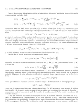
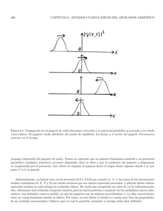

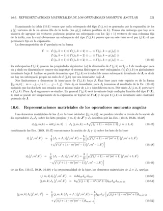
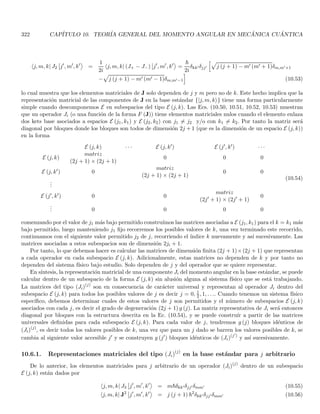
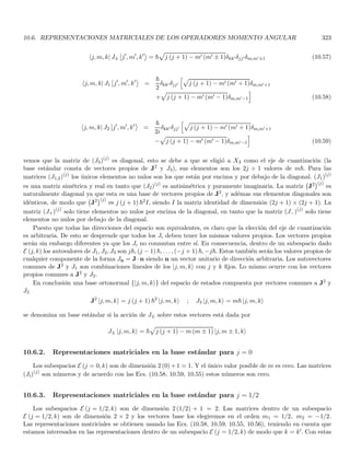
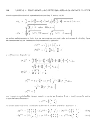
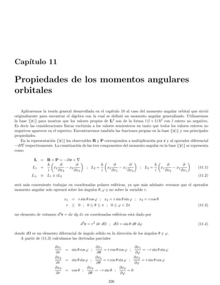
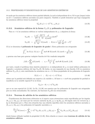
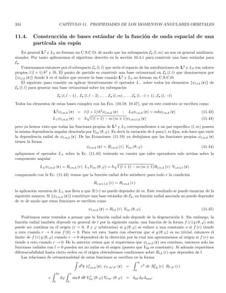
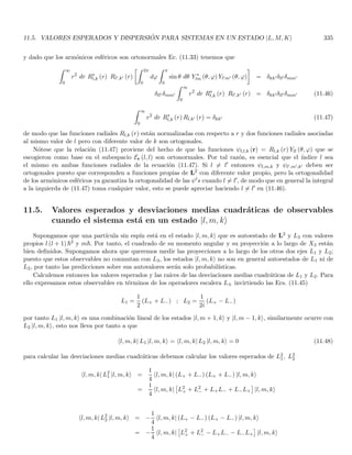
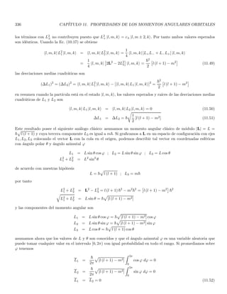
![1.43. THE CONTINUOUS BASES |Ri AND |Pi 101
of great importance are the commutators among the components Pi, Ri. We shall calculate them in the {|ri}
representation, for instance
hr| [X, Px] |ψi = hr| (XPx − PxX) |ψi = hr| (XPx) |ψi − hr| (PxX) |ψi
= hr| X |Pxψi − hr| Px |Xψi = x hr| Pxψi −
~
i
∂
∂x
hr| Xψi
= x hr| Px |ψi −
~
i
∂
∂x
hr| X |ψi =
~
i
x
∂
∂x
hr| ψi −
~
i
∂
∂x
[x hr| ψi]
=
~
i
x
∂
∂x
hr| ψi −
~
i
x
∂
∂x
[hr| ψi] −
~
i
hr| ψi
so that
hr| [X, Px] |ψi = i~ hr| ψi
since this is valid for any ket |ψi and any generalized ket |ri of the basis, we conclude that
[X, Px] = i~I
it is usual to omit the identity operator since it is not important for practical calculations. In a similar way, we
can calculate the other commutators, to condense notation it is convenient to define
R1 ≡ X, R2 ≡ Y, R3 ≡ Z, P1 ≡ Px, P2 ≡ Py, P3 ≡ Pz
to write
[Ri, Rj] = [Pi, Pj] = 0 ; [Ri, Pj] = i~δij (1.193)
they are called canonical commutation relations. These relations are intrinsic and should not depend on the basis
in which we derive them.
We can show that R and P are hermitian operators. For example let us show that X is hermitian
hϕ| X |ψi =
Z
d3
r hϕ |ri hr| X |ψi =
Z
d3
r ϕ∗
(r) x ψ (r) =
Z
d3
r ψ (r)∗
x ϕ (r)
∗
hϕ| X |ψi = hψ| X |ϕi∗
since this is valid for arbitrary kets |ψi and |ϕi, and taking into account Eq. (1.163) we conclude that X = X†.
For Px we see that
hϕ| Px |ψi =
Z
d3
p hϕ |pi hp| Px |ψi =
Z
d3
p ϕ̄∗
(p) px ψ̄ (p) =
Z
d3
p ψ̄ (p)∗
px ϕ̄ (p)
∗
hϕ| Px |ψi = hψ| Px |ϕi∗
and Px = P†
x. The procedure is the same for the other components of R and P
R = R†
, P = P†
There is an alternative proof of the hermiticity of P by using its action in the {|ri} representation given by
Eq. (1.191). Integrating Eq. (1.192) by parts we have
hϕ| Px |ψi =
~
i
Z
dy dz
Z ∞
−∞
dx ϕ∗
(r)
∂
∂x
ψ (r)
=
~
i
Z
dy dz
[ϕ∗
(r) ψ (r)]x=∞
x=−∞ −
Z ∞
−∞
dx ψ (r)
∂
∂x
ϕ∗
(r)](https://image.slidesharecdn.com/cuantica-220626164623-64979fb3/85/cuantica-pdf-343-320.jpg)
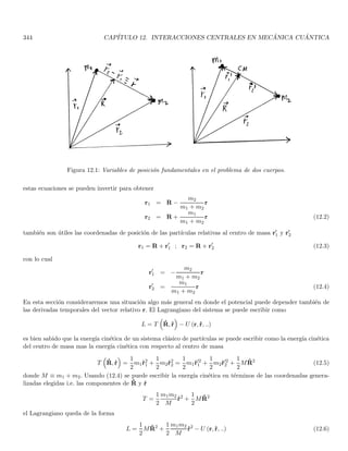
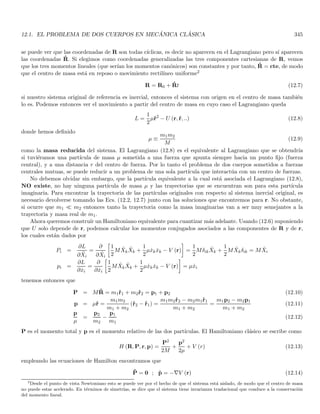

![104 CAPÍTULO 1. LINEAR OR VECTOR SPACES
substituting Eq. (1.200) in Eq. (1.198) we have
ψ (p) = 2π
1
2π~
3/2 Z ∞
0
r2
dr ψ (r)
2~
pr
sin
pr
~
thus, Eq. (1.196) is obtained.
1.44. General properties of two conjugate observables
Two arbitrary observables Q and P are called conjugate if they obey the conmutation rule
[Q, P] = i~ (1.201)
such couples of observables are frequently encountered in quantum mechanics. The position and momentum
observables are good examples. However, in what follows all properties are derived from the commutation rule
(1.201) regardless the specific form of the operators. Let us define the operator S (λ) that depends on a real
parameter λ as
S (λ) = e−iλP/~
(1.202)
since P is observable and so hermitian this operator is unitary
S†
(λ) = eiλP/~
= S−1
(λ) = S (−λ) (1.203)
since P obviously commute with itself, Eq. (1.149) leads to
S (λ) S (µ) = S (λ + µ) (1.204)
now we calculate the commutator [Q, S (λ)]. To do it, we take into account that [Q, P] = i~ clearly commutes
with Q and P, therefore we can apply theorem 1.70, Eq. (1.136) to obtain
[Q, S (P)] = [Q, P] S′
(P) = i~
−
iλ
~
e−iλP/~
= λS (P)
where we have written S (P) instead of S (λ) to emphasize that when applying Eq. (1.136) we are considering S
as a function of the operator P (so the derivative is with respect to P). Rewriting it in the old notation we have
[Q, S (λ)] = λS (λ) ⇒ QS (λ) − S (λ) Q = λS (λ)
QS (λ) = S (λ) [Q + λ] (1.205)
1.44.1. The eigenvalue problem of Q
Suppose that Q has a non-zero eigenvector |qi, with eigenvalue q
Q |qi = q |qi (1.206)
applying Eq. (1.205) on the vector |qi we have
QS (λ) |qi = S (λ) [Q + λ] |qi = S (λ) [q + λ] |qi
Q [S (λ) |qi] = [q + λ] [S (λ) |qi] (1.207)
therefore, S (λ) |qi is also an eigenvector of Q with eigenvalue q + λ. Note that S (λ) |qi is non-zero because S (λ)
is unitary so the norm of |qi is preserved. On the other hand, since λ can take any real value, we conclude that by](https://image.slidesharecdn.com/cuantica-220626164623-64979fb3/85/cuantica-pdf-360-320.jpg)
![1.44. GENERAL PROPERTIES OF TWO CONJUGATE OBSERVABLES 105
starting with an eigenvector of Q, we can construct another eigenvector of Q with any real eigenvalue by applying
the appropiate S (λ). Consequently, the spectrum of Q is continuous and consists of all real values.
Note that this result shows in particular that conjugate operators Q, P cannot exist in finite dimensional vector
spaces since for the latter the spectrum must be finite. Even they do not exist strictly in spaces of denumerable
dimension such as L2, (for which the spectrum must be at most denumerable), so the eigenvectors |qi will form
hyperbasis in L2.
Let us now show that if any given q is non-degenerate, then all the other eigenvalues of Q are also non-
degenerate. For this we assume that the eigenvalue q+λ is at least two-fold degenerate and arrive to a contradiction.
From this hypothesis, there are at least two orthogonal eigenvectors |q + λ, αi and |q + λ, βi associated with the
eigenvalue q + λ
hq + λ, β |q + λ, αi = 0 (1.208)
now consider the two vectors S (−λ) |q + λ, αi and S (−λ) |q + λ, βi from Eq. (1.207) we see that
QS (−λ) |q + λ, αi = [q + λ + (−λ)] S (−λ) |q + λ, αi = qS (−λ) |q + λ, αi
QS (−λ) |q + λ, βi = [q + λ + (−λ)] S (−λ) |q + λ, βi = qS (−λ) |q + λ, βi
so S (−λ) |q + λ, αi and S (−λ) |q + λ, βi are two eigenvectors associated with the eigenvalue q. Calculating the
inner product of them
hq + λ, β| S†
(−λ) S (−λ) |q + λ, αi = hq + λ, β |q + λ, αi = 0
where we have used Eq. (1.208) and the fact that S (λ) is unitary. Thus, we arrive to the fact that S (−λ) |q + λ, αi
and S (−λ) |q + λ, βi are two orthogonal (and so linearly independent) eigenvectors associated with q, contradicting
the hypothesis that q is non-degenerate. This result can be extended to find that the eigenvalues of Q must all
have the same degree of degeneracy.
We now look for the eigenvectors. We fix the relative phses of the diffrent eigenvectors of Q with respect to
the eigenvector |0i associated with the eigenvalue 0, by setting
|qi ≡ S (q) |0i (1.209)
applying S (λ) on both sides of (1.209) and using (1.204), we get
S (λ) |qi = S (λ) S (q) |0i = S (λ + q) |0i = |q + λi
and the corresponding bra gives
hq| S†
(λ) = hq + λ|
now using Eq. (1.203) we see that S† (λ) = S (−λ) from which
hq| S (−λ) = hq + λ| ⇒ hq| S (λ) = hq − λ|
where we have replaced λ → −λ in the last step. In summary the action of S (λ) on the eigenvectors |qi of Q are
given by
S (λ) |qi = |q + λi ; hq| S (λ) = hq − λ| (1.210)
now we can characterize the action of the operators P, Q and S (λ) in either the {|qi} basis or the {|pi} basis.
1.44.2. The action of Q, P and S (λ) in the {|qi} basis
Since Q is an observables the set of eigenvectors {|qi} of Q forms a basis. A given ket |ψi in our Hilbert space
can be written in the {|qi} basis as
ψ (q) ≡ hq |ψi](https://image.slidesharecdn.com/cuantica-220626164623-64979fb3/85/cuantica-pdf-361-320.jpg)
![108 CAPÍTULO 1. LINEAR OR VECTOR SPACES
and I is the identity matrix. Let |ψ±i be two linearly independent eigenvectors of K
K |ψ±i = κ± |ψ±i (1.217)
applying the ket |ψ±i on Eq. (1.216) we have
H |ψ±i =
1
2
(H11 + H22) I |ψ±i +
1
2
(H11 − H22) K |ψ±i
H |ψ±i =
1
2
[(H11 + H22) + (H11 − H22) κ±] |ψ±i
therefore |ψ±i are also eigenvectors of H with eigenvalues
H |ψ±i = E± |ψ±i ; E± ≡
1
2
[(H11 + H22) + (H11 − H22) κ±] (1.218)
note that the problem reduces to find the eigenvectors of K (which coincide with the ones of H) and also its
eigenvalues (which are related with the eigenvalues of H through Eq. 1.218). Solving the problem for K is equivalent
to choose the origin of the eigenvalues in (H11 + H22) /2 = (TrH)/2. Note that this shift is independent of the
basis chosen to write H.
1.45.2. Eigenvalues and eigenvectors of K
For simplicity we define the angles θ, ϕ in terms of the matrix elements Hij as follows
tan θ =
2 |H21|
H11 − H22
, 0 ≤ θ π (1.219)
H21 = |H21| eiϕ
, 0 ≤ ϕ 2π (1.220)
so ϕ is the argument of the term H21. Matrix K in Eq. (1.216) can be written as
K =
1 2|H21|e−iϕ
(H11−H22)
2|H21|eiϕ
(H11−H22) −1
!
=
1 tan θ e−iϕ
tan θ eiϕ −1
(1.221)
the characteristic equation of matrix (1.221) yields
det [K − λI] = 0 = (1 − κ) (−1 − κ) − tan2
θ ⇒
κ2
− 1 − tan2
θ = 0 ⇒ κ2
= 1 + tan2
θ =
1
cos2 θ
the eigenvalues of K read
κ+ =
1
cos θ
, κ− = −
1
cos θ
(1.222)
and they are real as expected. We can express 1/ cos θ in terms of the matrix elements Hij by using Eqs. (1.219)
and the fact that cos θ and tan θ are both of the same sign since 0 ≤ θ π.
1
cos θ
=
p
1 + tan2 θ =
s
1 +
4 |H21|2
(H11 − H22)2 =
s
(H11 − H22)2
+ 4 |H21|2
(H11 − H22)2
κ± = ±
1
cos θ
= ±
s
(H11 − H22)2
+ 4 |H21|2
(H11 − H22)2 (1.223)](https://image.slidesharecdn.com/cuantica-220626164623-64979fb3/85/cuantica-pdf-364-320.jpg)
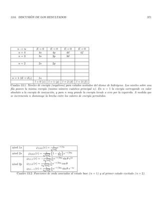
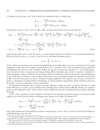
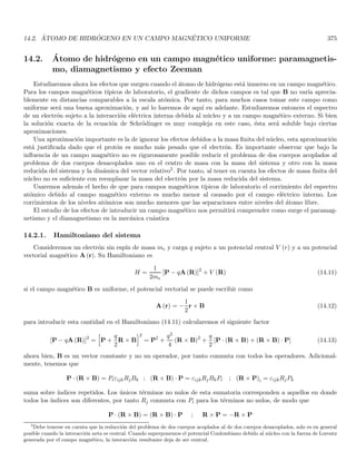
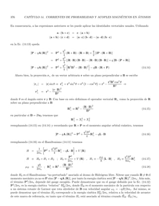
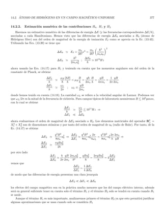
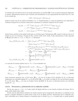
![110 CAPÍTULO 1. LINEAR OR VECTOR SPACES
an analogous calculation gives the eigenvector of K corresponding to κ− = −1/ cos θ
|ψ−i = − sin
θ
2
e−iϕ/2
|ϕ1i + cos
θ
2
eiϕ/2
|ϕ2i (1.227)
the eigenvalues of H are obtained by combining Eqs. (1.218, 1.223)
E± ≡
1
2
[(H11 + H22) + (H11 − H22) κ±]
=
1
2
(H11 + H22) ± (H11 − H22)
s
(H11 − H22)2
+ 4 |H21|2
(H11 − H22)2
#
E± ≡
1
2
(H11 + H22) ±
q
(H11 − H22)2
+ 4 |H21|2
it worths saying that the eigenvalue problem can be solved directly without resorting to the angles θ and ϕ defined
in Eq. (1.219, 1.220). This procedure is advantageous only if we have to calculate the eigenvectors as well.
1.45.3. Eigenvalues and eigenvectors of H
Let us summarize our results. We consider an hermitian operator R in a two dimensional Hilbert space, and
its matrix representation in the orthonormal basis {|ϕ1i , |ϕ2i}
H ≡
hϕ1| R |ϕ1i hϕ1| R |ϕ2i
hϕ2| R |ϕ1i hϕ2| R |ϕ2i
=
H11 H12
H21 H22
(1.228)
its eigenvalues and eigenvectors are given by
E± ≡
1
2
(H11 + H22) ±
q
(H11 − H22)2
+ 4 |H21|2
(1.229)
|ψ+i = cos
θ
2
e−iϕ/2
|ϕ1i + sin
θ
2
eiϕ/2
|ϕ2i (1.230)
|ψ−i = − sin
θ
2
e−iϕ/2
|ϕ1i + cos
θ
2
eiϕ/2
|ϕ2i (1.231)
tan θ =
2 |H21|
H11 − H22
, H21 = |H21| eiϕ
; 0 ≤ θ π , 0 ≤ ϕ 2π (1.232)
as a matter of consistence we can see that
E+ + E− = H11 + H22 = TrH , E+E− = H11H22 − |H12|2
= det H
in agreement with Eq. (1.93, 1.94). From Eq. (1.229), the spectrum becomes degenerate i.e. E+ = E− when
(H11 − H22)2
+ 4 |H21|2
= 0. That is when H11 = H22 and H12 = H21 = 0. So a 2 × 2 hermitian matrix has a
degenerate spectrum if and only if it is proportional to the identity.
It worths remarking that although functions of θ are expressed simply in terms of the Hij elements by means of
Eqs. (1.232), it is not the case when functions of θ/2 appears. Thus, when we do calculations with the eigenvectors
(1.230, 1.231), it is convenient to keep the results in terms of θ/2 up to the end of the calculation instead of
replacing it in terms of the Hij quantities.](https://image.slidesharecdn.com/cuantica-220626164623-64979fb3/85/cuantica-pdf-384-320.jpg)
![Capı́tulo 2
Construcción fenomenológica de los
postulados de la mecánica cuántica
Nuestro presente entendimiento de la naturaleza requiere reevaluar las leyes de la mecánica clásica, especial-
mente en lo referente a los fenómenos atómicos y subatómicos. No obstante, existen manifestaciones macroscópicas
de los procesos cuánticos. A manera de ejemplo, la existencia misma de los sólidos solo se puede explicar en un
contexto cuántico, y los modelos sobre calor especı́fico de los sólidos no se pueden explicar con un modelo clásico.
A finales del siglo diecinueve, se identificaban en la fı́sica dos tipos de entidades bien diferenciadas: la materia y
la radiación. Las leyes de Newton permitı́an explicar los fenómenos relativos a la materia en la escala macroscópica
y las ecuaciones de Maxwell proporcionaban una excelente descripción de la dinámica de la radiación1. Finalmente,
la interacción de la materia con la radiación la proporcionaba la ley de fuerza de Lorentz. Es notable el hecho
de que la teorı́a de Maxwell habia logrado la unificación de fenómenos que antes se consideraban separados: la
electricidad, el magnetismo y la óptica.
No obstante, a finales del siglo diecinueve y principios del veinte una serie de experimentos condujeron a
reevaluar la estructura fundamental de la materia y además a replantear las leyes que rigen a estas estructuras
fundamentales. La mecánica cuántica es entonces el resultado de estos replanteamientos. Vale decir por supuesto
que al menos en principio, el mundo macroscópico también se rige por la leyes de la cuántica, si bien para la
mayorı́a de fenómenos a escala humana, la Fı́sica clásica representa una descripción mucho más simple y al mismo
tiempo bastante adecuada.
A continuación se realizará una breve descripción de los experimentos que dieron lugar a las nuevas ideas sobre
el mundo microscópico, con el fin de dejar claros los puntos que es necesario reevaluar en la mecánica clásica. La
descripción de estos experimentos no pretende ser completa ni exhaustiva, solo pretende mostrar las ideas que
éstos nos arrojan sobre el comportamiento de la naturaleza a nivel microscópico (atómico y subatómico). Para un
estudio más detallado de estos experimentos el lector puede recurrir a los textos estándar sobre Fı́sica Moderna
(ver por ejemplo Ref. [1]).
2.1. La radiación del cuerpo negro
Un cuerpo negro tiene la capacidad de absorber toda la radiación que incide sobre él, a su vez esto lo convierte
en un emisor perfecto. Utilizando argumentos de la termodinámica y la mecánica estadı́stica, Rayleigh y Jeans
predijeron el espectro del cuerpo negro utilizando la distribución de Boltzmann. Sin embargo, las predicciones de
Rayleigh y Jeans estaban muy lejos del espectro experimental en el régimen de longitudes de onda corta, fenómeno
conocido como la “catástrofe del ultravioleta”. Es bien conocido que la energı́a asociada a una frecuencia particular
de la radiación del cuerpo negro se relaciona con la energı́a de una partı́cula cargada en la pared de una cavidad
del cuerpo negro oscilando sinusoidalmente a la misma frecuencia. Originalmente, Max Planck cuantizó la energı́a
1
Las ondas mecánicas podı́an explicarse en último término con las leyes de Newton.
111](https://image.slidesharecdn.com/cuantica-220626164623-64979fb3/85/cuantica-pdf-385-320.jpg)
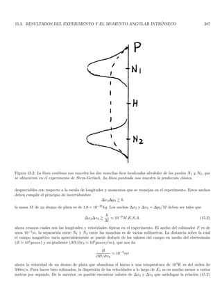
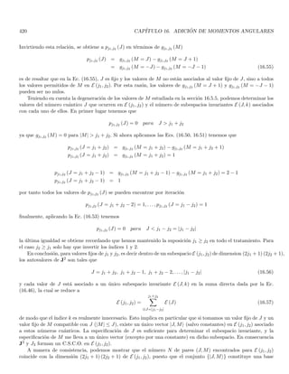
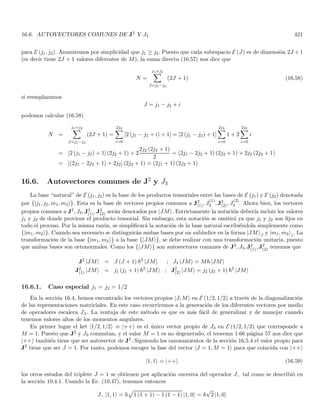
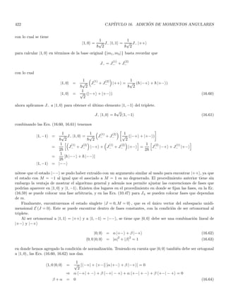
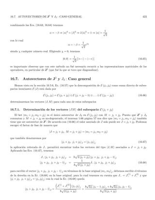
![138 CAPÍTULO 2. CONSTRUCCIÓN FENOMENOLÓGICA DE LOS POSTULADOS
(i.e. homogénea) la solución más simple (monocromática) es la solución tipo onda plana
ψ (r, t) = Aei(k·r−ωt)
(2.52)
es inmediato ver que la onda plana es tal que
|ψ (r, t)|2
= |A|2
de modo que si efectivamente representa a la onda asociada a una partı́cula libre, nos predice que la distribución
de probabilidad de una partı́cula libre es uniforme en el espacio, lo cual es compatible con la homogeneidad e
isotropı́a del espacio. Podrı́a argumentarse que las ondas planas no son de cuadrado integrable de modo que no
representan estrictamente un estado fı́sico. Sin embargo, nuestra experiencia con la óptica en la cual las ondas
planas tampoco son estados fı́sicos nos muestra que el estudio de sus propiedades es muy provechoso, por un lado
porque se puede considerar como el lı́mite de un estado fı́sico y por otro lado porque los estados fı́sicos se podrán
escribir como superposición de tales funciones en virtud de su completez (ver sección 1.31.1).
Tomaremos entonces la solución (2.52) como el prototipo de una onda piloto. Nuestro objetivo será realizar
una teorı́a no relativista que sea compatible con los postulados de De Broglie. Partiremos entonces de la relación
no relativista entre E y p para una partı́cula
E =
p2
2m
(2.53)
y utilizando las relaciones de De Broglie (2.49) llegamos a
ω =
~k2
2m
(2.54)
la relación de dispersión (2.54) nos dice que la ecuación de onda NO es la ecuación dinámica que gobierna a la
teorı́a cuántica no relativista de una partı́cula, ya que es fácil demostrar que insertando (2.52) en la ecuación de
onda clásica se obtiene la relación de dispersión
ω2
= k2
v2
(2.55)
siendo v la velocidad de la onda. Volveremos sobre este problema más adelante, de momento asumiremos que la
onda viajera libre (2.52) es solución de la ecuación de movimiento para el estado cuántico ψ de una partı́cula libre
con relación de dispersión dada por (2.54). Puesto que las ondas piloto deben generar los fenómenos ondulatorios,
es necesario que la combinación lineal de soluciones sea solución de la ecuación dinámica para generar los fenómenos
de interferencia.
2.11.1. Estados cuánticos arbitrarios como superposición de ondas planas
De acuerdo con lo anterior, y dado que las ondas planas pueden generar cualquier función de cuadrado integrable
(completez) cualquier estado cuántico de una partı́cula (no necesariamente libre) se puede escribir como una
superposición de la forma
ψ (r, t) =
1
(2π)3/2
Z
ψ̄ (k, t) ei[k·r−ωt]
d3
k (2.56)
donde d3k = dkx dky dkz representa un diferencial de volumen en el espacio de las k′s (usualmente denominado
espacio recı́proco). La transformada de Fourier ψ̄ (k) puede ser compleja pero debe ser bien comportada para
permitir derivar la solución dentro de la integral. Por supuesto, las transformadas de Fourier especı́ficas dependerán
del problema especı́fico.
Una función de onda que es superposición de ondas planas como la descrita en (2.56) se denomina un paquete
de ondas tridimensional. Por simplicidad, tomaremos el caso unidimensional
ψ (x, t) =
1
√
2π
Z
ψ̄ (k, t) ei[kx−ωt]
dk (2.57)
y estudiaremos más adelante el caso tridimensional. En primer lugar estudiaremos el perfil del paquete de onda
en un instante dado](https://image.slidesharecdn.com/cuantica-220626164623-64979fb3/85/cuantica-pdf-436-320.jpg)
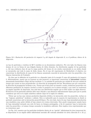
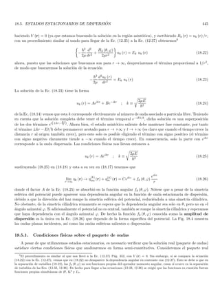
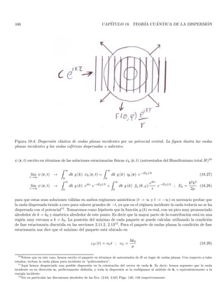
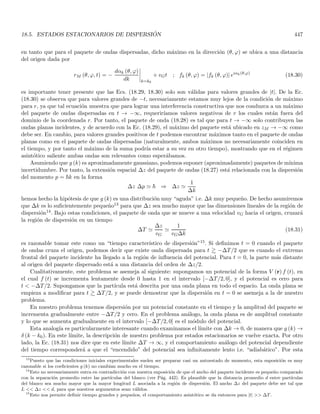
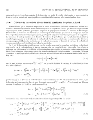
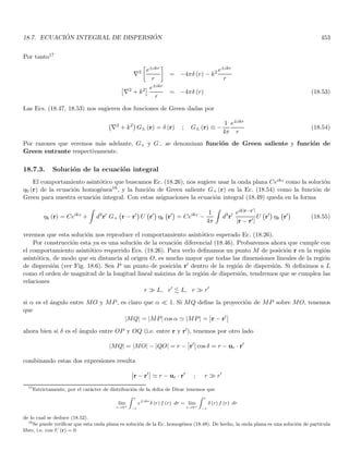
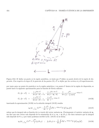
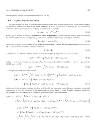
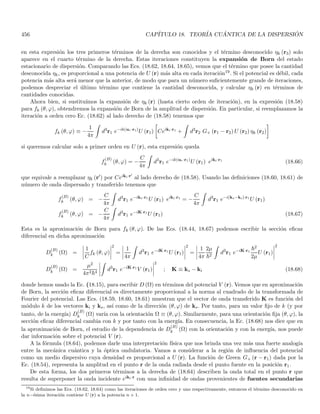
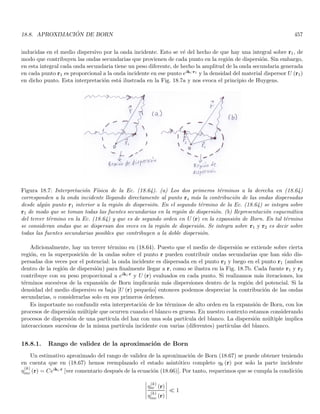
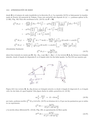
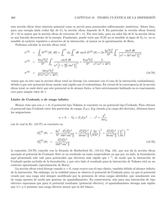
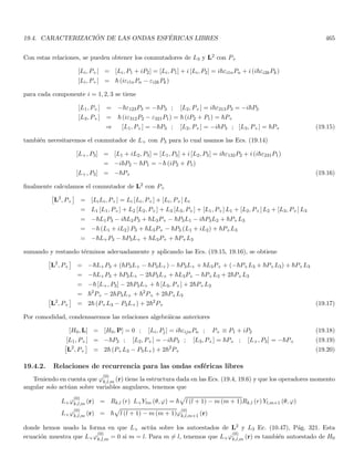
![eiα(k)
(2.63)
ahora asumamos que α (k) varı́a lentamente en el intervalo [k0 − ∆k/2, k0 + ∆k/2] donde la longitud del fasor](https://image.slidesharecdn.com/cuantica-220626164623-64979fb3/85/cuantica-pdf-466-320.jpg)
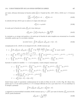
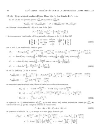
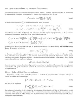
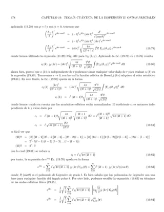
![e
i
h
α(k0)+(k−k0)[dα
dk ]k=k0
+kx
i
dk
=
1
√
2π
Z k0+ ∆k
2
k0− ∆k
2](https://image.slidesharecdn.com/cuantica-220626164623-64979fb3/85/cuantica-pdf-479-320.jpg)
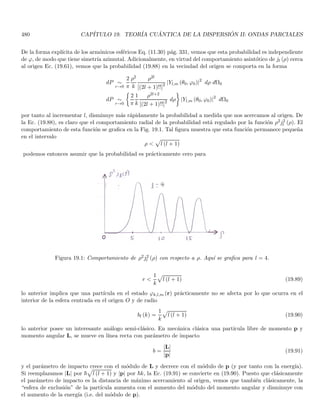
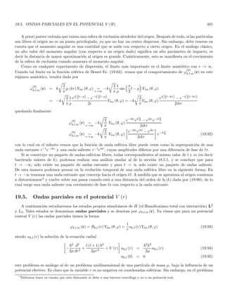
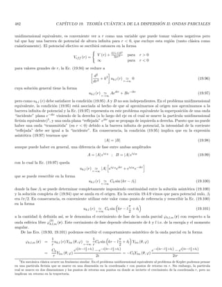
![e
i
h
α(k0)+(k−k0)[dα
dk ]k=k0
+kx−k0x+k0x
i
dk
=
1
√
2π
Z k0+ ∆k
2
k0− ∆k
2](https://image.slidesharecdn.com/cuantica-220626164623-64979fb3/85/cuantica-pdf-483-320.jpg)
![e
i
h
α(k0)+(k−k0)[dα
dk ]k=k0
+(k−k0)x+k0x
i
dk
=
ei[α(k0)+k0x]
√
2π
Z k0+ ∆k
2
k0− ∆k
2](https://image.slidesharecdn.com/cuantica-220626164623-64979fb3/85/cuantica-pdf-487-320.jpg)
![e
i
n
(k−k0)
[dα
dk ]k=k0
+x
o
dk (2.66)
quedando finalmente
ψ (x, 0) ≃
ei[k0x+α(k0)]
√
2π
Z k0+ ∆k
2
k0− ∆k
2](https://image.slidesharecdn.com/cuantica-220626164623-64979fb3/85/cuantica-pdf-491-320.jpg)
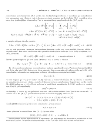
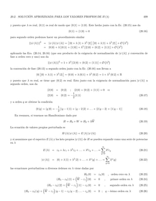
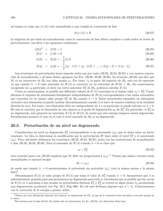
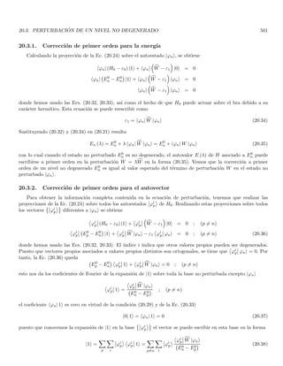
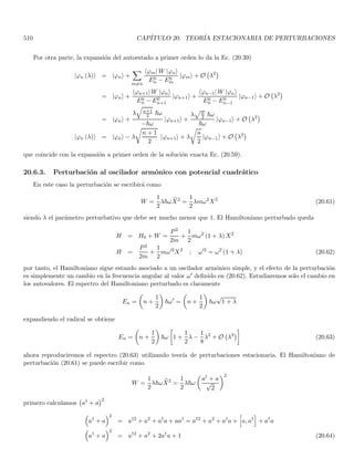
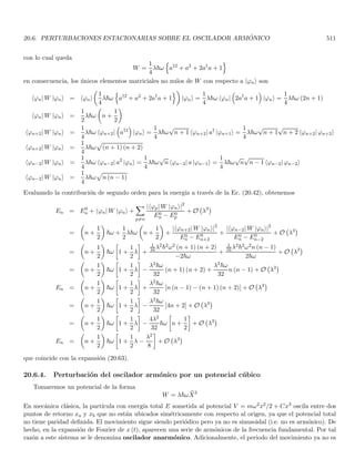
![(Fig. 2.6b), y en el proceso de integración
la fase se mantiene casi constante, por tanto la interferencia es constructiva y |ψ (x, 0)| es máximo.
De otra parte, la Ec. (2.69) se convierte en una igualdad para la posición xM tal que xM = x0, en cuyo caso no
hay oscilación y la interferencia es completamente constructiva. Por tanto, la posición xM (0) = x0 corresponde al
centro del paquete de onda (máximo del módulo del paquete) que de acuerdo con la Ec. (2.68) viene dada por:
xM (0) = x0 = −
dα
dk
k=k0
(2.70)
alternativamente, se puede ver que (2.70) nos da la posición del centro del paquete teniendo en cuenta que la Ec.
(2.58) adquiere su máximo en valor absoluto cuando las ondas de mayor amplitud (aquellas con k cercano a k0)
interfieren constructivamente. Esto ocurre cuando las fases que dependen de k de estas ondas varı́an lentamente
alrededor de k0. Para obtener el centro del paquete se impone que la derivada con respecto a k de la fase sea cero
para k = k0, esta fase se puede ver en la segunda igualdad de la Ec. (2.65) y se obtiene
d
dk
[kx + α (k)]k=k0
= 0 ⇒
x +
dα
dk
k=k0
= 0 (2.71)
vemos entonces que la condición de fase estacionaria (2.71) se reduce a (2.70).
Cuando x se aleja de x0, el valor de |ψ (x, 0)| decrece. El propósito ahora es definir un ancho ∆x dependiendo
del decrecimiento de |ψ (x, 0)| alrededor de x0. Nótese que este decrecimiento es apreciable si ei(k−k0)(x−x0) oscila
una vez o más cuando k recorre el dominio desde k0 − ∆k
2 hasta k0 + ∆k
2 es decir cuando
∆k · |x − x0| 2π
donde hemos definido el “umbral” para |x − x0| como el valor para el cual se ejecuta una oscilación. Si definimos
∆x ≡ |x − x0| /2π como el ancho tı́pico del paquete, tenemos
∆k ∆x 1 (2.72)](https://image.slidesharecdn.com/cuantica-220626164623-64979fb3/85/cuantica-pdf-512-320.jpg)
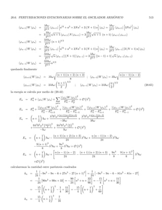
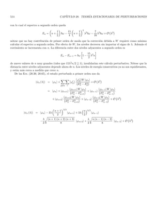
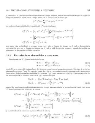
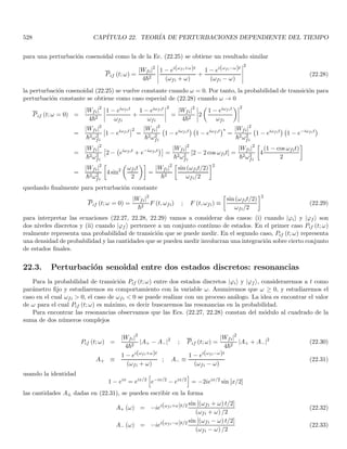
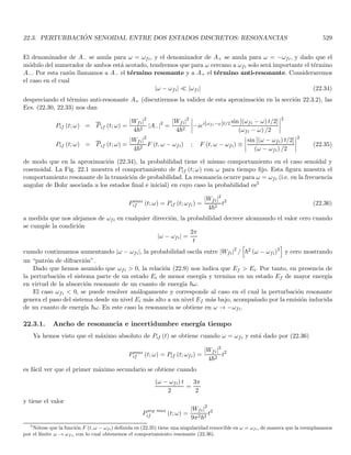
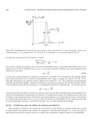
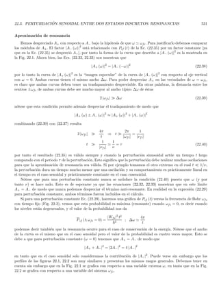
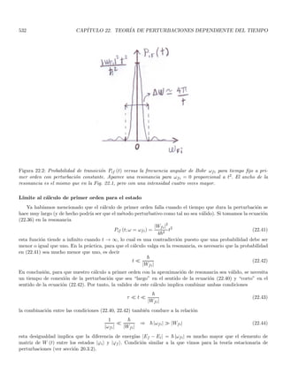
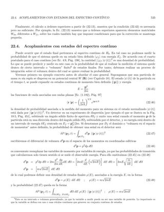
![2
dp
dP (x, 0) representa la probabilidad de encontrar a la partı́cula en t = 0 en el intervalo [x, x + dx]. Similarmente,
dP̄ (p, 0) es la probabilidad de obtener una medida del momento de la partı́cula en t = 0 que esté dentro del
intervalo [p, p + dp].
Ahora escribamos la desigualdad (2.72) en términos de E y p usando la relaciones de De Broglie (2.49)
∆x ∆p ~ (2.73)
para dar una interpretación fı́sica a (2.73), supongamos que el estado de una partı́cula está definido por el paquete
de onda (2.57). En tal caso, la probabilidad de encontrar la partı́cula en t = 0 dentro del intervalo [x0 − ∆x/2,
x0 + ∆x/2] es prácticamente uno. Decimos entonces que ∆x es la incertidumbre en la medida de la posición de
la partı́cula. Similarmente, si medimos el momento de la partı́cula en el mismo tiempo (t = 0) tal probabilidad es
casi uno dentro del intervalo [p0 − ∆p/2, p0 + ∆p/2]. Es decir que ∆p mide la incertidumbre en la determinación
del momento de la partı́cula.
A la luz de lo anterior la Ec. (2.73) expresa que es imposible medir al mismo tiempo la posición y el momento
de la partı́cula con grado arbitrario de exactitud. Cuando alcanzamos el lı́mite inferior en (2.73) una disminución
en ∆x (es decir un aumento en la exactitud de la medición de la posición) conduce a un aumento en ∆p (es decir
un aumento en la incertidumbre de la medida del momento, o equivalentemente una disminución en la exactitud
de tal medida) y viceversa. Este enunciado se conoce como el principio de incertidumbre de Heisenberg.
Notemos que el valor del término de la derecha en (2.73) nos expresa más bien un orden de magnitud que un
lı́mite inferior preciso.
Es de anotar que si bien hay un análogo clásico del principio de incertidumbre para las ondas, no hay un análogo
clásico para las partı́culas. En realidad hemos visto que el principio de incertidumbre está asociado inicialmente a
los parámetros de onda, que se conectan a los parámetros de partı́cula por medio de las relaciones de De Broglie,
estas a su vez están asociadas a la dualidad onda partı́cula que es una caracterı́stica cuántica. La pequeñez de ~
hace que este principio de incertidumbre no se manifieste en los sistemas macroscópicos.
9
En otras palabras, es más usual medir parámetros de materia que parámetros de onda.](https://image.slidesharecdn.com/cuantica-220626164623-64979fb3/85/cuantica-pdf-534-320.jpg)
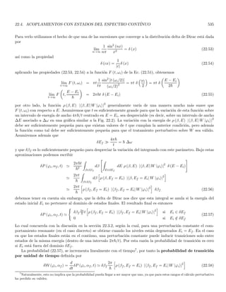
![148 CAPÍTULO 2. CONSTRUCCIÓN FENOMENOLÓGICA DE LOS POSTULADOS
Volviendo a nuestro caso de onda monocromática cuántica, si usamos las Ecs. (2.78, 2.54) vemos que la
velocidad de fase está dada por
Vf (k) =
ω
k
=
~k2
2mk
=
~k
2m
(2.79)
de modo que Vf es función explı́cita de k. Nótese que si usáramos la relación de dispersión dada por la ecuación
de onda, Ec. (2.55) entonces Vf no presentarı́a dispersión (Vf no depende de k) como ocurre efectivamente con
las ondas clásicas libres (como las ondas electromagnéticas libres).
Ahora analizaremos el caso de ondas que son superposición de ondas planas. Veremos a continuación que
cuando las diferentes ondas tienen diferentes velocidades de fase, la velocidad del máximo xM del paquete de onda
no es la velocidad de fase promedio dada por
ω0
k0
=
~k0
2m
como antes, comencemos con el ejemplo simple de la superposición de tres ondas planas similares a las descritas
en (2.60) pero ahora con variación temporal
ψ (x, t) =
g (k0)
√
2π
ei(k0x−ω0t)
+
1
2
ei[(k0− ∆k
2 )x−(ω0− ∆ω
2 )t] +
1
2
ei[(k0+ ∆k
2 )x−(ω0+ ∆ω
2 )t]
(2.80)
=
g (k0)
√
2π
ei(k0x−ω0t)
1 + cos
∆k
2
x −
∆ω
2
t
ψ (x, t) =
g (k0)
√
2π
e
ik0
x−
ω0
k0
t
1 + cos
∆k
2
x −
∆ω
∆k
t
(2.81)
puesto que las tres ondas tiene números de onda k0 y k0 ± ∆k, es claro que k0 es el número de onda promedio.
Similarmente, ω0 es la frecuencia angular promedio.
De la Ec. (2.81) se vé claramente que el máximo de |ψ (x, t)| que estaba en x = 0 cuando t = 0 está ahora en
el punto
xM (t) =
∆ω
∆k
t (2.82)
y no en el punto x = ω0t/k0. El origen de este resultado se puede apreciar en la Fig. 2.8, en (a) se representa la
Figura 2.8: Posición de tres máximos consecutivos (1) (2) (3) para cada una de las tres ondas planas de la super-
posición en la Ec. (2.81). (a) Configuración de los máximos en t = 0, para el cual hay interferencia constructiva
en x = 0, que se da con los máximos rotulados por (2). (b) Configuración en un instante posterior en el cual la
interferencia totalmente constructiva se da a la derecha de x con los máximos (3).
posición en t = 0 de tres máximos consecutivos de cada una de las partes reales de las tres ondas. Puesto que los](https://image.slidesharecdn.com/cuantica-220626164623-64979fb3/85/cuantica-pdf-538-320.jpg)
![2.13. EVOLUCIÓN TEMPORAL DE PAQUETES DE ONDAS LIBRE 149
máximos denotados con (2) coinciden en x = 0, hay una interferencia constructiva en este punto lo cual nos da
el máximo de |ψ (x, t = 0)|. Puesto que la velocidad de fase aumenta con k según (2.79), tenemos que el máximo
(3) de la onda k0 + ∆k
2 termina alcanzando al máximo de la onda k0 también denotado por tres. Similarmente
el máximo (3) de k0 alcanzará al máximo de k0 − ∆k
2 denotado por (3). Un análisis detallado muestra que todos
coinciden en cierto tiempo t, determinando entonces el máximo xM (t) de |ψ (x, t)| por interferencia constructiva.
El cálculo detallado del punto donde esto ocurre reproduce la Ec. (2.82).
Analicemos finalmente el caso en el cual el paquete de ondas es arbitrario y consta de una superposición
contı́nua de ondas planas como en la Ec. (2.57). El corrimiento del centro del paquete se encuentra aplicando de
nuevo el método de fase estacionaria. Comparando la forma de ψ (x, t) con la de ψ (x, 0) Ecs. (2.57, 2.58) vemos
que si la transformada de Fourier en (2.57) no depende explı́citamente del tiempo, entonces ψ (x, t) se obtiene
a partir de ψ (x, 0) con la asignación ψ̄ (k) → ψ̄ (k) e−iω(k)t. Por tanto, el razonamiento dado en la pág. 142 se
mantiene válido reemplazando el argumento α (k) de ψ̄ (k) en la Ec. (2.63), por el argumento
α (k) → α (k) − ω (k) t (2.83)
la condición de fase estacionaria (2.71) se escribe ahora de la forma
d
dk
[kxM + α (k) − ω (k) t]k=k0
= 0 ⇒
xM +
dα
dk
−
dω (k)
dk
t
k=k0
= 0
Y la dinámica del centro del paquete estará dada por
xM (t) =
dω
dk
k=k0
t −
dα
dk
k=k0
que nos reproduce una vez más el resultado (2.82) solo que en este caso ∆ω y ∆k tienden a cero ya que hay un
barrido contı́nuo en estas variables. La velocidad del máximo del paquete de ondas es
Vg (k0) =
dxM (t)
dt
=
dω
dk
k=k0
conocida como velocidad de grupo del paquete. Con la relación de dispersión (2.54) para partı́cula libre y teniendo
en cuenta (2.79) tenemos que
Vg (k0) =
~k0
m
= 2Vf (k0) (2.84)
Notamos entonces dos diferencias importantes entre la onda asociada a la partı́cula libre cuántica y la solución
libre ondulatoria proveniente de la ecuación de onda. (a) Las ondas electromagnéticas clásicas libres no presentan
dispersión en tanto que la solución cuántica (ondulatoria) de partı́cula libre si presenta dispersión y (b) para
las ondas electromagnéticas libres la velocidad de grupo es menor que la de fase, mientras que para la solución
ondulatoria de partı́cla libre cuántica, la velocidad de grupo es mayor que la velocidad de fase10.
Nótese que el resultado (2.84) reproduce adecuadamente el lı́mite clásico ya que si ∆x y ∆p son ambos
despreciables, podemos hablar de la posición xM (t) y del momento p0 de la partı́cula. Pero entonces su velocidad
debe ser p0/m según la mecánica clásica, esto es compatible con la Ec. (2.84) obtenida en el marco cuántico con
p0 = ~k0, siempre que ∆x y ∆p sean ambos despreciables Vg se puede asociar a la velocidad de la partı́cula, que
es la velocidad del máximo del paquete.
Es posible también estudiar la forma en que evoluciona la forma del paquete. Si por ejemplo ∆p es una
constante de movimiento entonces ∆x se incrementa con el tiempo, (dipersión del paquete).
10
Nótese que el hecho de que la velocidad de grupo sea mayor a la de fase en la Ec. (2.84), no entra en contradicción con la relatividad,
puesto que nuestros resultados solo son válidos en un régimen no relativista, ya que la relación de dispersión (2.54) proviene de la
ecuación (2.53), la cual es no relativista.](https://image.slidesharecdn.com/cuantica-220626164623-64979fb3/85/cuantica-pdf-539-320.jpg)
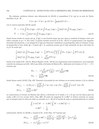
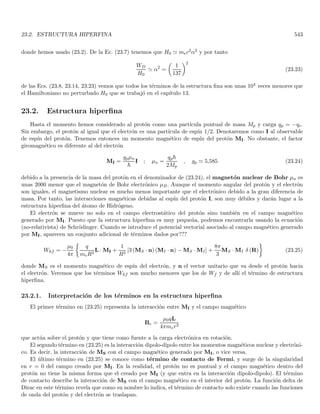
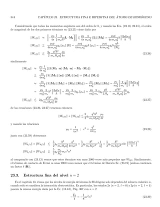
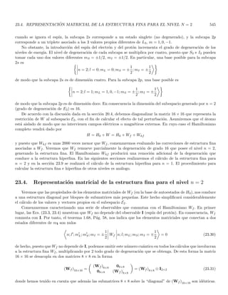
![152 CAPÍTULO 2. CONSTRUCCIÓN FENOMENOLÓGICA DE LOS POSTULADOS
especı́fico en que el paquete inicial posee el perfil gaussiano dado por la Ec. (2.87), se tiene que
ψ (x, t) =
√
a
(2π)3/4
Z ∞
−∞
e− a2
4
(k−k0)2
ei[kx−ω(k)t]
dk ; ω (k) =
~k2
2m
(2.93)
veremos que el paquete permanece gaussiano para todo tiempo t. Se puede agrupar la parte dependiente de k de
los exponentes para formar un cuadrado perfecto, con el fin de comparar (2.93) con (2.85) y obtener
ψ (x, t) =
2a2
π
1/4
eiϕ
a4 + 4~2t2
m2
1/4
eik0x
exp
−
h
x − ~k0
m t
i2
a2 + 2i~t
m
ϕ ≡ −θ −
~k2
0
2m
t ; tan 2θ =
2~
ma2
t
el módulo al cuadrado del paquete (densidad de probabilidad) en el tiempo t está dado por
|ψ (x, t)|2
=
r
2
πa2
1
q
1 + 4~2t2
m2a4
exp
−
2a2
x − ~k0
m t
2
a4 + 4~2t2
m2
(2.94)
debemos ahora calcular Z ∞
−∞
|ψ (x, t)|2
dx (2.95)
una forma serı́a empleando (2.85) para integrar (2.94). No obstante, es más simple observar de la expresión (2.93)
que la transformada de Fourier de ψ (x, t) viene dada por
ψ̄ (k, t) = e−iω(k)t
ψ̄ (k, 0) (2.96)
se vé entonces que](https://image.slidesharecdn.com/cuantica-220626164623-64979fb3/85/cuantica-pdf-550-320.jpg)

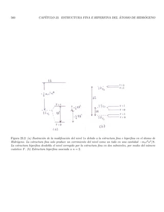
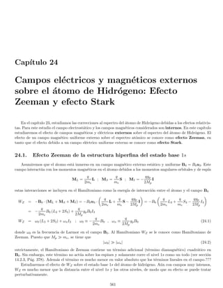
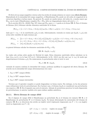
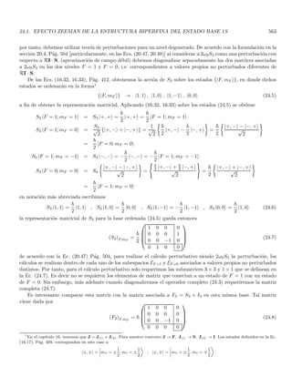
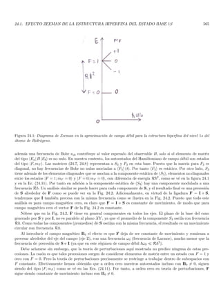
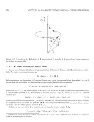
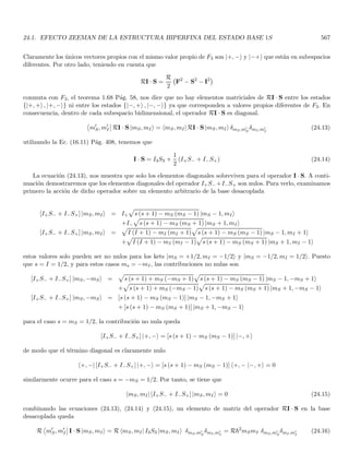
![156 CAPÍTULO 3. ECUACIÓN DE SCHRÖDINGER Y SUS PROPIEDADES
Ahora bien, teniendo en cuenta que
k ≡ 2πK ; ω ≡ 2πν
la velocidad de grupo queda
Vg =
dω
dk
=
dν
dK
=
p dp
mh
h
dp
=
p
m
= vpartı́cula
y podemos reescribir las relaciones de De Broglie en la forma
p = ~k ; E = ~ω (3.3)
si insertamos estas relaciones en (3.2) obtenenemos la siguiente relación de Dispersión
~2k2
2m
+ V (x, t) = ~ω (3.4)
tomaremos como prototipo la ecuación para la partı́cula libre con potencial constante. Las consideraciones ante-
riores nos dicen que la ecuación de movimiento que genere la función de onda ψ (x, t) (i.e. la dinámica de las ondas
piloto), debe cumplir las siguientes propiedades
1. Debe ser consistente con las Ecs. (3.1, 3.2). Es decir debe cumplir los postulados de De Broglie y la relación
no relativista entre E y p.
2. Debe ser lineal y homogénea en ψ (x, t) con el fin de que sea válido el principio de superposición que a su vez
nos genera los fenómenos ondulatorios de interferencia. Esto implica que si ψ1 (x, t) y ψ2 (x, t) son soluciones
de la ecuación una combinación lineal de ellas también es solución.
3. En general, consideraremos potenciales que solo dependen de la posición y el tiempo V = V (x, t). Cuando
el potencial es constante la partı́cula es libre y por tanto se deben conservar E y p, lo cual a su vez implica
que se conservan λ = 2π/k y ν de acuerdo con las relaciones (3.1).
4. Las soluciones para partı́cula libre son funcionalmente idénticas a las soluciones de la ecuación de onda
homogénea, pero deben cumplir con una relación de dispersión que sea consistente con la Ec. (3.4) con
V constante, en vez de la relación de dispersión para ondas libres dada por (2.55), lo cual nos dice que
la ecuación de onda no es la ecuación dinámica para la función de onda ψ (r, t). Entonces la ecuación de
movimiento para partı́cula libre debe tener soluciones en forma de ondas viajeras con número de onda y
frecuencia constantes.
5. Lo anterior nos lleva a postular que funciones de onda de la forma Aei(kx−ωt) son soluciones para partı́cula
libre (i.e. con potencial constante), ya que estas funciones son soluciones de la ecuación de onda homogénea
que corresponden a ondas viajeras con número de onda y frecuencia constantes, y que gracias a las relaciones
de De Broglie, también corresponden a momento y energı́a conservados.
La linealidad y homogeneidad prohibe términos del tipo [ψ (x, t)]2
(no lineales) o términos independientes de
ψ (x, t) (términos inhomogéneos o fuentes). Puesto que la mayorı́a de ecuaciones dinámicas de la Fı́sica son a lo
más de segundo orden, postularemos que los términos lineales son a lo más de segundo orden en el espacio y el
tiempo, y posiblemente un término lineal en ψ (x, t). Parametrizaremos a la ecuación en la forma siguiente
a1
∂ψ (x, t)
∂x
+ a2
∂2ψ (x, t)
∂x2
− b1
∂ψ (x, t)
∂t
− b2
∂2ψ (x, t)
∂t2
+ c ψ (x, t) = 0
asumamos que la solución de partı́cula libre es ψ (x, t) = Aei(kx−ωt), además se debe cumplir la relación de
dispersión (3.4) con V constante. Esta relación de dispersión contiene un término proporcional a k2 que se obtendrı́a
de una segunda derivada espacial de la onda plana, y un término lineal en ω que se puede extraer de una primera](https://image.slidesharecdn.com/cuantica-220626164623-64979fb3/85/cuantica-pdf-582-320.jpg)
![3.1. PLAUSIBILIDAD DE LA ECUACIÓN DE SCHRÖDINGER 157
derivada temporal de la onda plana. La ausencia de un término lineal en k y de un término cuadrático en ω
sugiere la ausencia de primeras derivadas espaciales y de segundas derivadas temporales. Finalmente, la presencia
del potencial en (3.4) sugiere la presencia de un término lineal en ψ de la forma V ψ. El ansatz para la solución se
reduce a
a2
∂2ψ (x, t)
∂x2
+ V ψ (x, t) = b1
∂ψ (x, t)
∂t
(3.5)
ahora debemos ajustar los parámetros a2 y b1 de manera que exista una solución tipo onda plana que reproduzca
la relación de dispersión (3.4). Recordemos que en mecánica clásica, el carácter complejo de las soluciones de la
ecuación de onda se introduce solo por conveniencia y la solución Fı́sica es la parte real de la solución compleja.
Por este motivo si bien podemos insertar una solución tipo onda plana en (3.5), es razonable intentar primero usar
la solución real para la ecuación de onda clásica como prototipo de solución, insertaremos entonces una función
de onda de la forma
ψ (x, t) = cos (kx − ωt) (3.6)
teniendo en cuenta que k, ω y V son constantes, se tiene que
∂2ψ (x, t)
∂x2
= −k2
cos (kx − ωt) ;
∂ψ
∂t
= ω sin (kx − ωt)
y al insertar estos resultados en (3.5) obtenemos
−a2k2
cos (kx − ωt) + V cos (kx − ωt) = b1ω sin (kx − ωt)
V − a2k2
cos (kx − ωt) = b1ω sin (kx − ωt)
pero no es posible ajustar los parámetros para que esta relación sea válida para todo x, t, de modo que la solución
clásica dada por (3.6) no es compatible con la relación de dispersión de la teorı́a. Aún podemos tratar de encontrar
una solución real si agregamos una fase adicional en la forma cos (kx − ωt + δ) que es equivalente a escribir una
solución de la forma
ψ (x, t) = cos (kx − ωt) + γ sin (kx − ωt) (3.7)
lo cual también se puede postular observando que en tal caso ambas derivadas tendrán senos y cosenos que
permitirán igualar coeficientes adecuadamente
∂2ψ (x, t)
∂x2
= −k2
cos (kx − ωt) − γk2
sin (kx − ωt) ;
∂ψ
∂t
= ω sin (kx − ωt) − γω cos (kx − ωt)
que al insertarlos en (3.5) nos da
−a2k2
[cos (kx − ωt) + γ sin (kx − ωt)] + V [cos (kx − ωt) + γ sin (kx − ωt)]
= b1ω [sin (kx − ωt) − γ cos (kx − ωt)]
quedando
−a2k2
+ V + b1ωγ
cos (kx − ωt) + −a2k2
γ + V γ − b1ω
sin (kx − ωt) = 0
Los coeficientes de seno y coseno deben anularse para que esta relación sea válida para todo x, t. Tenemos
entonces dos ecuaciones con tres incógnitas (a2, b1, γ) que junto con la relación de dispersión (3.4), nos da
−a2k2
+ V + b1ωγ = 0 ; −a2k2
γ + V γ − b1ω = 0 ;
~2k2
2m
+ V = ~ω (3.8)
las dos primeras ecuaciones se pueden reescribir como
−a2k2
+ V = −b1ωγ ; −a2k2
+ V =
b1
γ
ω ⇒ −b1ωγ =
b1
γ
ω
⇒ −γ =
1
γ
⇒ γ2
= −1](https://image.slidesharecdn.com/cuantica-220626164623-64979fb3/85/cuantica-pdf-583-320.jpg)
![3.2. ECUACIÓN DE SCHRÖDINGER CON POTENCIAL ESCALAR INDEPENDIENTE DEL TIEMPO 159
dividiendo a ambos lados por χ (t) ϕ (r) se escribe
−
~2
2m
∇2ϕ (r)
ϕ (r)
+ V (r) = i~
1
χ (t)
∂χ (t)
∂t
el miembro izquierdo solo depende de la posición en tanto que el derecho depende solo del tiempo. Por tanto
ambos miembros deben ser iguales a una constante que por comodidad la tomaremos como ~ω, de momento ω es
solo una constante a ajustar, aunque es claro que debe tener dimensiones de frecuencia angular. Tenemos entonces
que
i~
1
χ (t)
∂χ (t)
∂t
= ~ω ⇒
∂χ (t)
∂t
= −iωχ (t)
χ (t) = Ae−iωt
(3.13)
y la ecuación para la parte espacial es
−
~2
2m
∇2ϕ (r)
ϕ (r)
+ V (r) = ~ω ⇒
−
~2
2m
∇2
ϕ (r) + V (r) ϕ (r) = ~ωϕ (r) (3.14)
combinando las Ecs. (3.12, 3.13), la solución para la ecuación de Schrödinger (3.11) es
ψ (r, t) = ϕ (r) e−iωt
(3.15)
donde hemos absorbido el factor A en la solución ϕ (r) de la ecuación (3.14).
Nótese que la solución (3.15) nos conduce a una densidad de probabilidad independiente del tiempo, aunque
inhomogénea
|ψ (r, t)|2
= |ϕ (r)|2
razón por la cual se conoce como solución estacionaria de la ecuación de Schrödinger. Ahora bien, la Ec.
(3.15) nos muestra que la constante de integración ω corresponde efectivamente a la frecuencia angular asociada
a la función de onda estacionaria. Nótese que en la solución estacionaria, solo aparece un valor de frecuencia
angular ω que a su vez nos conduce a un valor bien definido de la energı́a de acuerdo con la relación de Planck
Einstein E = ~ω. En mecánica clásica un potencial independiente del tiempo nos lleva a la conservación de la
energı́a total. En mecánica cuántica, lo que podemos decir es que para potenciales independientes del tiempo
existen estados de energı́a bien determinada. La Ec. (3.14) se puede escribir entonces como
−
~2
2m
∇2
+ V (r)
ϕ (r) = Eϕ (r) (3.16)
que se puede reescribir como
Hϕ (r) = Eϕ (r) ; H ≡ −
~2
2m
∇2
+ V (r) (3.17)
siendo H un operador diferencial que es claramente lineal
H [λ1ϕ1 (r) + λ2ϕ2 (r)] = λ1Hϕ1 (r) + λ2Hϕ2 (r)
y vemos que (3.17) es una ecuación de valores propios para el operador H en la cual ϕ (r) son las funciones propias
(vectores propios) y las energı́as E son los valores propios. Las energı́as permitidas para la partı́cula son entonces
los valores propios del operador H. Nótese que no cualquier solución ϕ (r) de la ecuación de Schrödinger es una
solución fı́sica, debemos imponer que sea de cuadrado integrable, esta imposición restringirá los valores permitidos
de energı́a y nos llevará a una cuantización de esta cantidad.](https://image.slidesharecdn.com/cuantica-220626164623-64979fb3/85/cuantica-pdf-585-320.jpg)
![3.3. PROPIEDADES GENERALES DE LA ECUACIÓN DE SCHRÖDINGER 163
para todo tiempo, de modo que PT representa una “carga generalizada” que se conserva. Por supuesto esto no
significa que la distribución de esta “carga” (distribución de probabilidad), permanezca igual en el tiempo para
cada punto r, las variaciones de ρ (r, t) con el tiempo generan una propagación de la distribución de carga. En
general tanto las variaciones espaciales como temporales de ρ (r, t) generan una corriente de probabilidad, si ρ
no es función del tiempo se genera una corriente estacionaria. Recordemos que el volumen no es necesariamente
todo el espacio si existen regiones con probabilidad cero. Lo importante es que no cruce corriente de probabilidad
en la superficie que delimita al volumen de integración, ya que si esto ocurre, habrá probabilidad diferente de cero
en regiones que en tiempos anteriores eran inaccesibles. Esta situación es análoga al caso en que ρ (r, t) simbolizaba
una densidad de carga eléctrica a la cual le podemos asociar una densidad de corriente J (r, t).
Es bien conocido que la conservación global de la carga generalizada proviene de una ley de conservación local
que prohibe la creación espontánea de carga generalizada neta. Esto implica que si tomamos un volumen por cuya
superficie limitadora cruza corriente de carga generalizada, el flujo neto de carga por la superficie hacia afuera
(adentro) debe estar compensado por una disminución (aumento) en la carga interior al volumen, el enunciado
preciso de esta ley local de conservación es
∂
∂t
ρ (r, t) + ∇ · J (r, t) = 0 (3.28)
siendo ρ la densidad de carga generalizada y J la densidad de corriente generalizada, esta expresión es conocida
como ecuación de continuidad. Puesto que hemos encontrado la carga conservada (probabilidad total) y definido
ya la densidad de probabilidad, debemos encontrar una densidad de corriente de probabilidad que nos dé una
ecuación de la forma (3.28), en este caso estamos tratando a la probabilidad como un fluı́do o medio contı́nuo.
Volveremos a la ecuación de Schrödinger en representación de coordenadas dado por (3.10)
−
~2
2m
∇2
ψ (r, t) + V (r, t) ψ (r, t) = i~
∂ψ (r, t)
∂t
(3.29)
el potencial V (r, t) debe ser real para que H sea hermı́tico (lo cual es esencial para la conservación de la proba-
bilidad como ya vimos). La ecuación compleja conjugada de la Ec. de Schrödinger es
−
~2
2m
∇2
ψ∗
(r, t) + V (r, t) ψ∗
(r, t) = −i~
∂ψ∗ (r, t)
∂t
(3.30)
multiplicamos (3.29) por ψ∗ (r, t) y (3.30) por −ψ (r, t) y sumamos
−
~2
2m
ψ∗
(r, t) ∇2
ψ (r, t) + V (r, t) ψ∗
(r, t) ψ (r, t) = i~ψ∗
(r, t)
∂ψ (r, t)
∂t
~2
2m
ψ (r, t) ∇2
ψ∗
(r, t) − V (r, t) ψ (r, t) ψ∗
(r, t) = i~ψ (r, t)
∂ψ∗ (r, t)
∂t
quedando
−
~2
2m
ψ∗
∇2
ψ − ψ∇2
ψ∗
= i~
ψ∗ ∂ψ
∂t
+ ψ
∂ψ∗
∂t
−
~
2mi
ψ∗
∇2
ψ − ψ∇2
ψ∗
=
∂
∂t
[ψ∗
ψ]
sumando y restando un término a la izquierda
−
~
2mi
ψ∗
∇2
ψ + (∇ψ∗
) · (∇ψ) − (∇ψ∗
) · (∇ψ) − ψ∇2
ψ∗
=
∂
∂t
[ψ∗
ψ]
−
~
2mi
∇ · [ψ∗
∇ψ − ψ∇ψ∗
] =
∂ρ
∂t](https://image.slidesharecdn.com/cuantica-220626164623-64979fb3/85/cuantica-pdf-589-320.jpg)
![164 CAPÍTULO 3. ECUACIÓN DE SCHRÖDINGER Y SUS PROPIEDADES
quedando finalmente
∂ρ
∂t
+ ∇ ·
~
2mi
[ψ∗
∇ψ − ψ∇ψ∗
]
= 0 (3.31)
y comparando (3.31) con la ecuación (3.28) de continuidad se tiene que
J =
~
2mi
[ψ∗
∇ψ − ψ∇ψ∗
]
esta ecuación se puede reescribir definiendo
J =
~
m
1
2i
[Z − Z∗
]
; Z ≡ ψ∗
∇ψ
J =
1
m
1
2
~Z
i
+
~Z
i
∗
=
1
m
Re
~Z
i
de modo que
J (r, t) =
~
2mi
[ψ∗
∇ψ − ψ∇ψ∗
] =
1
m
Re
ψ∗
~
i
∇ψ
(3.32)
hemos probado entonces la conservación local de la probabilidad y encontramos la forma explı́cita de la densidad
de corriente, la cual es real como era de esperarse.
Vale la pena calcular la corriente de probabilidad para el caso especial de estados estacionarios de la forma
(3.15), en tal caso al reemplazar (3.15) en (3.32) resulta
J =
~
2mi
[ψ∗
∇ψ − ψ∇ψ∗
] =
~
2mi
n
ϕ (r) e−iωt
∗
∇
ϕ (r) e−iωt
−
ϕ (r) e−iωt
∇
ϕ (r) e−iωt
∗
o
J =
~
2mi
ϕ∗
(r) eiωt
e−iωt
∇ϕ (r) − ϕ (r) e−iωt
eiωt
∇ϕ∗
(r)
quedando finalmente
J (r) =
~
2mi
{ϕ∗
(r) ∇ϕ (r) − ϕ (r) ∇ϕ∗
(r)} =
1
m
Re
ϕ∗
(r)
~
i
∇ϕ (r)
estados estacionarios (3.33)
comparando, (3.32) con (3.33), vemos que para estados estacionarios, la corriente se puede calcular reemplazando
ψ (r, t) por ϕ (r), es decir omitiendo la componente temporal de ψ. Efectivamente, (3.33) corresponde a una
corriente estacionaria tal como se usa en mecánica clásica, i.e. una corriente que depende de la posición pero que
no depende explı́citamente del tiempo.
3.3.5. Expresión polar de la corriente de probabilidad
Consideremos una función de onda arbitraria ψ (r), utilizando su descomposición compleja polar tenemos
ψ (r) = α (r) eiξ(r)
; α (r) ≥ 0 , 0 ≤ ξ (r) 2π
si sustituı́mos esta expresión polar en la Ec. (3.32) para la densidad de corriente de probabilidad encontramos
que3
J (r) =
~
2mi
n
α (r) e−iξ(r)
∇
h
α (r) eiξ(r)
i
− α (r) eiξ(r)
∇
h
α (r) e−iξ(r)
io
=
~
2mi
n
α (r) e−iξ(r)
eiξ(r)
[∇α (r) + iα (r) ∇ξ (r)] − α (r) eiξ(r)
e−iξ(r)
[∇α (r) − iα (r) ∇ξ (r)]
o
J (r, t) =
~
m
α2
(r, t) ∇ξ (r, t) (3.34)
3
Por simplicidad hemos omitido la posible dependencia explı́cita del tiempo pero esto no altera los resultados.](https://image.slidesharecdn.com/cuantica-220626164623-64979fb3/85/cuantica-pdf-590-320.jpg)
![3.5. POTENCIALES RECTANGULARES, ANÁLOGO ÓPTICO 167
3.5.1. Estrategia de solución para potenciales acotados con discontinuidades de salto
Veamos ahora la estrategia especı́fica de solución para los estados estacionarios de la partı́cula sometidas a
potenciales discontı́nuos. En las regiones de energı́a potencial constante usamos la Ec. (3.38)
d2
dx2
+
2m
~2
(E − V )
ϕ (x) = 0 (3.43)
es útil distinguir tres casos
(a) E V , introduzcamos por conveniencia una constante positiva k definida por
E − V ≡
~2k2
2m
(3.44)
al reemplazar en (3.43) queda
d2
dx2
+ k2
ϕ (x) = 0 (3.45)
que es la ecuación de un oscilador armónico y la solución de la Ec. (3.45) se puede escribir como
ϕ (x) = Aeikx
+ A′
e−ikx
(3.46)
donde A y A′ son complejos constantes.
(b) E V , esta condición corresponde a regiones del espacio que están clásicamente prohibidas. En este caso
introducimos la constante positiva ρ dada por
V − E ≡
~2ρ2
2m
(3.47)
y la Ec. (3.43) queda
d2
dx2
− ρ2
ϕ (x) = 0 (3.48)
con solución
ϕ (x) = Beρx
+ B′
e−ρx
(3.49)
siendo B y B′ constantes complejas.
(c) E = V , en este caso
d2ϕ (x)
dx2
= 0 ⇒ ϕ (x) = Cx + C′
Ahora veamos el comportamiento de las soluciones en la discontinuidad. La primera tentación es pensar que
la función de onda debe ser discontı́nua en un punto donde el potencial lo sea, veremos sin embargo que tanto
ϕ (x) como dϕ (x) /dx deben ser contı́nuas y solo es la segunda derivada d2ϕ (x) /dx2 la que es discontı́nua en el
punto. Para ver esto, recordemos que un potencial con una discontinuidad de salto en x1 representa en fı́sica el
lı́mite cuando ε → 0 de un potencial Vε (x) que es igual a V (x) fuera del intervalo [x1 − ε, x1 + ε], pero que varı́a
de forma contı́nua en dicho intervalo. Consideremos la ecuación
d2
dx2
ϕε (x) +
2m
~2
[E − Vε (x)] ϕε (x) = 0 (3.50)
asumimos que Vε (x) está acotado en el intervalo [x1 − ε, x1 + ε], y que esta cota no depende del parámetro ε.
Esto se cumple en la mayorı́a de los casos, ya que usualmente Vε estará definido dentro de los valores [V0, V1] que
se tienen en la discontinuidad de salto a la izquierda y la derecha de x1. Escogemos una solución ϕε (x) que para
x x1 − ε y para x x1 + ε coincida con una solución dada de la Ec. (3.43). La idea es demostrar que cuando
ε → 0 entonces ϕε (x) tiende a una función ϕ (x) contı́nua y diferenciable a primer orden en x1. Es posible probar](https://image.slidesharecdn.com/cuantica-220626164623-64979fb3/85/cuantica-pdf-593-320.jpg)
![168 CAPÍTULO 3. ECUACIÓN DE SCHRÖDINGER Y SUS PROPIEDADES
a través de las propiedades de la ecuación diferencial (3.43) que ϕε (x) permanece acotada para cualquier valor
de ε con una cota independiente de ε, en la vecindad de x = x1. Esto fı́sicamente implica que la densidad de
probabilidad permanece finita. Integrando la Ec. (3.50) en el intervalo [x1 − η, x1 + η] resulta
Z x1+η
x1−η
d
dx
d
dx
ϕε (x)
dx +
2m
~2
Z x1+η
x1−η
[E − Vε (x)] ϕε (x) dx = 0
dϕε (x1 + η)
dx
−
dϕε (x1 − η)
dx
=
2m
~2
Z x1+η
x1−η
[Vε (x) − E] ϕε (x) dx (3.51)
y dado que Vε (x) y ϕε (x) permanecen acotados con cotas independientes de ε, la integral a la derecha de la Ec.
(3.51) tiende a cero cuando η tiende a cero. Por lo tanto
lı́m
η→0
dϕε (x1 + η)
dx
−
dϕε (x1 − η)
dx
= 0
por tanto, en este lı́mite, dϕ/dx es contı́nua en x = x1 y por tanto también ϕ (x) ya que derivabilidad implica
continuidad. Por otro lado, d2ϕ/dx2 es discontı́nua en x = x1 puesto que en la Ec. (3.43) vemos que
lı́m
η→0+
d2ϕ (x1 + η)
dx2
+
2m
~2
[E − V (x1 + η)] ϕ (x1 + η)
= 0
lı́m
η→0+
d2ϕ (x1 + η)
dx2
= lı́m
η→0+
2m
~2
{[V (x1 + η) − E] ϕ (x1 + η)}
lı́m
η→0+
d2ϕ (x1 + η)
dx2
=
2m
~2
{[V1 − E] ϕ (x1)}
siendo V1 el valor del potencial a la derecha de x1, similarmente
lı́m
η→0−
d2ϕ (x1 + η)
dx2
=
2m
~2
{[V0 − E] ϕ (x1)}
siendo V0 el valor del potencial a la izquierda de x1. Tenemos entonces que en x1 la segunda derivada presenta un
salto dado por
lı́m
η→0+
d2ϕ (x1 + η)
dx2
− lı́m
η→0−
d2ϕ (x1 + η)
dx2
=
2m
~2
(V1 − V0) ϕ (x1)
esto es una discontinuidad de salto para la segunda derivada ya que V1 6= V0. Nótese sin embargo, que la segunda
derivada permanece acotada. Es importante resaltar la importancia de que Vε (x) permanezca acotado. Por ejem-
plo, si V (x) = aδ (x) tenemos una función cuya integral permanece finita pero que no es acotada. En tal caso,
ϕ (x) permanece contı́nua pero no la primera derivada.
Por tanto, para encontrar la solución de los estados estacionarios cuando el potencial es contı́nuo a trozos
con discontinuidades de salto finito, calculamos primero las soluciones para las regiones en donde el potencial es
constante (con E V ó E V según el caso), y hacemos el “empalme” en los puntos donde hay discontinuidades
exigiendo la continuidad de la solución y de su primera derivada.
3.5.2. Expresión para la corriente en regiones de potencial constante
Por simplicidad consideraremos un problema unidimensional de una partı́cula colocada en un potencial cons-
tante V0. Aunque este caso corresponde a partı́cula libre, resulta interesante obtener la corriente en términos de
V0 ya que después consideraremos la posibilidad de regiones con potencial constante pero diferente en cada región.
Como la corriente (3.33) depende de la solución para la función de onda estacionaria debemos considerar varios
casos según la sección 3.5.1](https://image.slidesharecdn.com/cuantica-220626164623-64979fb3/85/cuantica-pdf-594-320.jpg)
![3.5. POTENCIALES RECTANGULARES, ANÁLOGO ÓPTICO 169
(a) E V0, en tal caso la solución estacionaria viene dada por la Ec. (3.46)
ϕ (x) = Aeikx
+ A′
e−ikx
(3.52)
donde hemos usado la definición (3.44)
E − V0 ≡
~2k2
2m
y sustituyendo (3.52) en la expresión (3.33) para la corriente
Jx =
~
2mi
[ϕ∗
∂xϕ − ϕ∂xϕ∗
]
Jx =
~
2mi
h
A∗
e−ikx
+ A′∗
eikx
∂x
Aeikx
+ A′
e−ikx
−
Aeikx
+ A′
e−ikx
∂x
A∗
e−ikx
+ A′∗
eikx
i
Jx =
~
2mi
h
A∗
e−ikx
+ A′∗
eikx
ikAeikx
− ikA′
e−ikx
−
Aeikx
+ A′
e−ikx
−ikA∗
e−ikx
+ ikA′∗
eikx
i
Jx =
~k
2m
h
A∗
e−ikx
+ A′∗
eikx
Aeikx
−
A∗
e−ikx
+ A′∗
eikx
A′
e−ikx
+
Aeikx
+ A′
e−ikx
A∗
e−ikx
−
Aeikx
+ A′
e−ikx
A′∗
eikx
i
Jx =
~k
2m
h
A∗
A + A′∗
Ae2ikx
− A∗
A′
e−2ikx
− A′∗
A′
+ AA∗
+ A′
A∗
e−2ikx
− AA′∗
e2ikx
− A′
A′∗
i
Jx =
~k
2m
h
2 |A|2
+ A′∗
Ae2ikx
− AA′∗
e2ikx
− A∗
A′
e−2ikx
+ A′
A∗
e−2ikx
− 2](https://image.slidesharecdn.com/cuantica-220626164623-64979fb3/85/cuantica-pdf-595-320.jpg)
![2
i
(3.53)
el signo relativo se puede entender teniendo en cuenta que la función de onda (3.52) representa dos ondas con
momentos opuestos p = ±~k con densidades de probabilidad |A|2
y |A′|2
, además ~k
m = p
m = vg nos dice que Jx es
de la forma ρvg como era de esperarse.
(b) Cuando E V0 la solución está dada por las Ecs. (3.47, 3.49)
ϕ (x) = Beρx
+ B′
e−ρx
(3.54)
V0 − E ≡
~2ρ2
2m
(3.55)
sustituyendo (3.54) en (3.33) nos da
Jx =
~
2mi
[ϕ∗
∂xϕ − ϕ∂xϕ∗
]
Jx =
~
2mi
B∗
eρx
+ B′∗
e−ρx
∂x Beρx
+ B′
e−ρx
− Beρx
+ B′
e−ρx
∂x B∗
eρx
+ B′∗
e−ρx
Jx =
~
2mi
B∗
eρx
+ B′∗
e−ρx
ρBeρx
− ρB′
e−ρx
− Beρx
+ B′
e−ρx
ρB∗
eρx
− ρB′∗
e−ρx
Jx =
~ρ
2mi
B∗
eρx
+ B′∗
e−ρx
Beρx
− B∗
eρx
+ B′∗
e−ρx
B′
e−ρx
− Beρx
+ B′
e−ρx
B∗
eρx
+ Beρx
+ B′
e−ρx
B′∗
e−ρx
Jx =
~ρ
2mi
B∗
Be2ρx
+ B′∗
B − B∗
B′
− B′∗
B′
e−2ρx
− BB∗
e2ρx
− B′
B∗
+ BB′∗
+ B′
B′∗
e−2ρx
Jx =
~ρ
2mi
B∗
Be2ρx
− BB∗
e2ρx
+ 2B′∗
B − 2B∗
B′
− B′∗
B′
e−2ρx
+ B′
B′∗
e−2ρx
Jx =
~ρ
2mi
2B′∗
B − 2B∗
B′](https://image.slidesharecdn.com/cuantica-220626164623-64979fb3/85/cuantica-pdf-603-320.jpg)