We express a problem from visual astronomy in terms of Geometric (Clifford) Algebra, then solve the problem by deriving expressions for the sine and cosine of the angle between projections of two vectors upon a plane. Geometric Algebra enables us to do so without deriving expressions for the projections themselves.

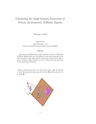
1. Calculating the Angle between Projections of
Vectors via Geometric (Clifford) Algebra
February 5, 2018
James Smith
nitac14b@yahoo.com
https://mx.linkedin.com/in/james-smith-1b195047
Abstract
We express a problem from visual astronomy in terms of Geometric
(Clifford) Algebra, then solve the problem by deriving expressions for the
sine and cosine of the angle between projections of two vectors upon a
plane. Geometric Algebra enables us to do so without deriving expressions
for the projections themselves.
“Derive expressions for the sine and cosine of the angle of rotation,
β, from the projection of u upon the bivector ˆM to the projection of
v upon ˆM.”
1

2. Contents
1 Introduction 2
2 Formulating the Problem in Geometric-Algebra (GA) Terms,
and Devising a Solution Strategy 3
2.1 Initial Observations . . . . . . . . . . . . . . . . . . . . . . . . . . 3
2.2 Recalling What We’ve Learned from Solving Similar Problems
via GA . . . . . . . . . . . . . . . . . . . . . . . . . . . . . . . . . 4
2.3 Further Observations, and Identifying a Strategy . . . . . . . . . 6
3 Solutions for cos β and sin β 8
3.1 Expressions for u · ˆM and v · ˆM . . . . . . . . . . . . . . . . . . 8
3.2 Expressions for u · ˆM and v · ˆM . . . . . . . . . . . . . . . . 9
3.3 Solution for sin β . . . . . . . . . . . . . . . . . . . . . . . . . . . 9
3.3.1 Expansion of u · ˆM v · ˆM 2 . . . . . . . . . . . . . . 10
3.3.2 Expansion of ˆM
−1
u · ˆM v · ˆM 2 . . . . . . . . . . . 10
3.3.3 Final result for sin β . . . . . . . . . . . . . . . . . . . . . 10
3.4 Solution for cos β . . . . . . . . . . . . . . . . . . . . . . . . . . . 11
4 Testing the Formulas that We’ve Derived 11
5 Conclusions, and Summary of the Formulas Derived Herein 12
6 Appendix: Calculating the Unit Bivector ˆM of a Plane Whose
Dual is the Vector ˆe 13
1 Introduction
In this document, we will solve—numerically as well as symbolically—a problem
of a type that can take the following concrete form, with reference to Fig.1:
“At a certain location on the Earth, a vertical pole casts a shadow
on a perfectly flat, horizontal plaza. On that plaza, local residents

3. Figure 1: A gnomon (vertical pole) casts a shadow on a perfectly flat, level
plaza. The direction of vector s is from the base of the gnomon to the tip of the
shadow. The direction of the Sun’s rays is ˆr. Upon the plaza, local inhabitants
have drawn a line pointing in the direction “local north” (ˆnL). The unit vector
in the direction of the plane’s normal is ˆg.
who are fans of naked-eye astronomy have traced a north-south
line running through the base of the pole. With respect to a right-
handed orthonormal reference frame with basis vectors ˆa, ˆb, and
ˆc, the direction of the Sun’s rays is given by the unit vector ˆr =
ˆara + ˆbrb + ˆcrc. The direction of the upward-pointing vector normal
to the plaza is ˆg = ˆaga + ˆbgb + ˆcgc, and the direction of the Earth’s
rotational axis (i.e., the direction from the center of the Earth to
the North Pole) is ˆnL = ˆanLa + ˆbnLb + ˆcnLc. What is the angle, β,
between the north-south line and the pole’s shadow?”
2 Formulating the Problem in Geometric-Algebra
(GA) Terms, and Devising a Solution Strategy
2.1 Initial Observations
Let’s begin by making a few observations that might be useful:
1. A vertical pole that is used to cast a shadow on a flat surface for the
purpose of astronomical observations is known as a gnomon. We’ll use
that term in the rest of this document.
2. By saying “the direction of the Sun’s rays is ˆr = ˆara + ˆbrb + ˆcrc”, we
assumed that all of the Sun’s rays are parallel. We’ll use that assumption
throughout this document.
3. For our purposes, the Earth can be assumed perfectly spherical.
3

4. Figure 2: The plaza is a plane tangent to the Earth (assumed spherical) at the
point at which the gnomon is embedded .
4. The plaza is a plane tangent to the Earth at the point at which the gnomon
is embedded (Fig. 2).
5. The direction of the shadow is the direction of the perpendicular projection
of ˆr upon the plaza. Fig. 2 shows why: the gnomon is perpendicular to
the plaza, so the shadow is the perpendicular projection some vector λˆr
upon the plaza. Thus, the direction from the base of the gnomon to the
tip of the shadow is the same as the direction of the projection of ˆr upon
the plaza.
6. The direction from south to north, as traced on the plaza by local residents,
is the perpendicular projection of ˆnc upon the plaza. As proof of that
assertion, consider Fig. 3. The south-north line on the plaza is tangent to
the great circle that passes through the Earth’s North Geographic Pole,
and that also passes through the base of the gnomon. The plane that
contains that great circle also contains the both ˆg and ˆnc. Therefore, that
plane is perpendicular to the plaza. Putting all of these ideas together,
the south-north line on the plaza is the projection of some scalar multiple
µˆnc of the vector ˆnc. Thus, that line has the direction of ˆnc’s projection
on the plaza.
2.2 Recalling What We’ve Learned from Solving Similar
Problems via GA
Let’s refresh our memory about techniques that we may used to solve other
problems via GA:
4

5. Figure 3: The direction “local north” (i.e., the direction from south to north, as
traced on the plaza by local residents) is the same as that of the perpendicular
projection of ˆnc upon the plaza.
1. Problems involving projections onto a plane are usually solved by using
the appropriately-oriented bivector that is parallel to the plane, rather
than by using the vector that is perpendicular to it. The Appendix
(Section 6) shows how to find the required bivector, given said vector. The
conclusion is that for the unit perpendicular vector ˆe = ˆaea + ˆbeb + ˆcec,
the appropriately-oriented unit bivector is
ˆM = ˆaˆbec + ˆbˆcea − ˆaˆceb (2.1)
In GA terms, ˆe is the “dual” of the bivector ˆM. We can also see that if
we write ˆM in the form ˆM = ˆaˆbmab + ˆbˆcmbc + ˆaˆcmac, then
mab = ec, mbc = ea, mac = −eb. (2.2)
2.
Notation: PC (d) is the
projection of d upon C.
The perpendicular projection of a given vector w upon a given unit
bivector, ˆM, is (Reference [1], p. 65 , and Ref. [2], p.119):
P ˆM (w) = w · ˆM ˆM
−1
. (2.3)
3. The inverse ˆM
−1
of the unit bivector ˆM is − ˆM .
4. For any vector y that is parallel to the bivector A, Ay = −yA.
5. Putting the last three observations, we arrive at
P ˆM (w) = ˆM w · ˆM . (2.4)
5

6. 6. If two vectors p and q are parallel to the bivector ˆM, then ˆpˆq = e
ˆMφ
, where
the scalar φ is the angle of rotation from p to q. Therefore, p · q + p ∧ q =
cos φ + ˆM sin φ. The algebraic sign of φ is positive if the direction of that
rotation is the same as the orientation of ˆM, and negative if in the opposite
direction.
7. Equating terms of the same grade in the previous item, we find that
cos φ = ˆp · ˆq;
sin φ = ˆM
−1
(ˆp ∧ ˆq) .
(2.5)
8. Macdonald’s definitions (Ref. [2], p. 101) of the inner and outer products
are often useful. Those definitions are, for a multivector A of grade j and
a multivector B of grade k:
Aj · Bk = AB k−j (Note: Aj · Bk does not exist if j > k);
Aj ∧ Bk = AB k+j.
(2.6)
2.3 Further Observations, and Identifying a Strategy
We ’ve been discussion how to find the angle between the south-north line and
the gnomon’s shadow. Now, to provide results that will be more generally useful,
we’ll treat two arbitrary vectors u and v (not necessarily unit vectors) and an
arbitrary unit bivector, ˆM (Fig. 4). We wish to find the sine and cosine of β,
the angle of rotation from P ˆM (u) to P ˆM (u).
We could solve the problem by calculating each of those projections according
to Eq. (2.3), then calculating the sine and cosine of the requested angle from Eq.
(2.5). However, our review of GA in the previous section suggests a strategy
that will save us considerable trouble. We’ll begin by using Eq. (2.3) to express
the two projections that interest us:
P ˆM (ˆu) = ˆu · ˆM ˆM
−1
;
P ˆM (v) = v · ˆM ˆM
−1
.
Can we now use Eq. (2.5) to calculate cos β and sin β? Not yet: although
u and v are unit vectors, their projects upon ˆM may not be. Therefore,
we’ll need to calculate P ˆM (u) and P ˆM (v) , a detail to which we’ll return
momentarily. First, we need to calculate u · ˆM ˆM
−1
· v · ˆM ˆM
−1
and
u · ˆM ˆM
−1
∧ v · ˆM ˆM
−1
.
The definitions of the inner and outer products in Eq. (2.6) use the product
AjBk, which in our case (because we want to know the rotation from P ˆM (u) to
P ˆM (u)) is
u · ˆM ˆM
−1
v · ˆM ˆM
−1
.
6

7. Figure 4: Diagram of the translation, into GA terms, of the more-general type of
problem that was motivated by our consideration of the specific case of shadows
cast upon a flat, horizontal plaza by a vertical pole. We’ll derive expressions for
the sine and cosine of the angle of rotation β from the projection of u upon the
bivector ˆM to the projection of v upon ˆM. The vector ˆe is the dual of ˆM, and
is therefore normal to ˆM.
7

8. Next, we recognize that v · ˆM is a vector, and is parallel to ˆM. Therefore,
using Eq. (2.4), we can write v · ˆM ˆM
−1
as ˆM v · ˆM . Using this idea in
the previous equation,
u · ˆM ˆM
−1
v · ˆM ˆM
−1
= u · ˆM ˆM
−1
ˆM v · ˆM
= u · ˆM v · ˆM . (2.7)
We could also find P ˆM (u)
and P ˆM (v) via a route
similar to that used in deriving
Eq. (2.7). For example,
P ˆM (u) = [P ˆM (u)]2
= u · ˆM ˆM
−1
u · ˆM ˆM
−1
= u · ˆM
2
= u · ˆM .
Now, let’s return to the question of P ˆM (u) and P ˆM (v) . Because
the vector P ˆM (u) is parallel to the unit bivector ˆM, P ˆM (u) ˆM is just a 90◦
rotation of P ˆM (u). Thus, P ˆM (u) ˆM = P ˆM (u) . But P ˆM (u) ˆM =
u · ˆM ˆM
−1
ˆM = u · ˆM. After using similar reasoning for P ˆM (v) , we find
that
P ˆM (u) = u · ˆM , and
P ˆM (v) = v · ˆM . (2.8)
Putting all of these ideas together, plus Eq. (2.5), and recognizing that
u · ˆM and v · ˆM are vectors (and therefore are of grade 1),
sin β =
ˆM
−1
u · ˆM v · ˆM 2
u · ˆM v · ˆM
, (2.9a)
cos β =
u · ˆM v · ˆM 0
u · ˆM v · ˆM
. (2.9b)
3 Solutions for cos β and sin β
We’ll begin by writing ˆM and the two vectors as
u = ˆaua + ˆbub + ˆcuc,
v = ˆava + ˆbvb + ˆcvc, and
ˆM = ˆaˆbmab + ˆbˆcmbc + ˆaˆcmac.
3.1 Expressions for u · ˆM and v · ˆM
Vector u is of grade 1, and bivector ˆM is of grade 2, so from Eq. (2.6),
u · ˆM = u ˆM 2−1
= ˆaua + ˆbub + ˆcuc ˆaˆbmab + ˆbˆcmbc + ˆaˆcmac 1
= ˆa (−ubmab − ucmac) + ˆb (uamab − ucmbc) + ˆc (uamac + ubmbc) .
8

9. Similarly,
v · ˆM = ˆa (−vbmab − vcmac) + ˆb (vamab − vcmbc) + ˆc (vamac + vbmbc) .
3.2 Expressions for u · ˆM and v · ˆM
Using the expressions that we developed in Section 3.1 , u · ˆM 2
and v · ˆM ,
plus the fact that m2
ab + m2
bc + m2
ac = 1 because ˆM is a unit bivector,
u · ˆM 2
= u2
a 1 − m2
bc + u2
b 1 − m2
ac + u2
c 1 − m2
ab
+ 2uaubmacmbc + 2ubucmabmac − 2uaucmabmbc ,
(3.1a)
and
v · ˆM 2
= v2
a 1 − m2
bc + v2
b 1 − m2
ac + v2
c 1 − m2
ab
+ 2vavbmacmbc + 2vbvcmabmac − 2vavcmabmbc .
(3.1b)
Using the correspondence (Eq. (2.2)) between coefficients in ˆM and ˆe, we
can also write Eq. (3.1) as
u · ˆM 2
= u2
a 1 − e2
a + u2
b 1 − e2
b + u2
c 1 − e2
c
− 2uaubeaeb − 2ubucebec − 2uauceaec ,
(3.2a)
and
v · ˆM 2
= v2
a 1 − e2
a + v2
b 1 − e2
b + v2
c 1 − e2
c
− 2vavbeaeb − 2vbvcebec − 2vavceaec .
(3.2b)
3.3 Solution for sin β
As you might expect, the expansion of Eq. (2.9)a becomes extensive and messy,
so we’ll do it in several steps.
9

10. 3.3.1 Expansion of u · ˆM v · ˆM 2
After considerable simplification, using the expressions developed in Section 3.1
for u · ˆM and v · ˆM,
u · ˆM v · ˆM 2 = ˆaˆb (uavb − ubva) m2
ab + (ubvc − ucvb) mabmbc
+ (uavc − ucva) mabmac ]
+ ˆbˆc (ubvc − ucvb) m2
bc + (uavb − ubva) mabmbc
+ (uavc − ucva) mbcmac ]
+ ˆaˆc (uavc − ucva) m2
ac + (uavb − ubva) mabmac
+ (ubvc − ucvb) mbcmac ] .
(3.3)
3.3.2 Expansion of ˆM
−1
u · ˆM v · ˆM 2
Surprisingly, left-multiplying the expression for u · ˆM v · ˆM 2 (Eq. (3.3))
by ˆM
−1
gives a comparatively simple result. The inverse of a unit bivector is
just the negative of that bivector, so ˆM
−1
= − ˆM = −ˆaˆbmab − ˆbˆcmbc − ˆaˆcmac.
After expanding, carrying out massive cancellations, and using the fact that
m2
ab + m2
bc + m2
ac = 1,
ˆM
−1
u · ˆM v · ˆM 2 = (uavb − ubva) mab + (ubvc − ucvb) mbc
+ (uavc − ucva) mac.
(3.4)
Does our answer make sense? The expression on the right-hand side of Eq. (3.4) will be the numerator
of the final expression for sin β. We should stop here to ask ourselves whether
that expression makes sense. For example, does it behave as it should, given the
physical situation for which it’s been derived? One thing we know is that if the
vectors u and v are reversed, then angle β will remain the same in magnitude,
but will change algebraic sign. The same is true for the right-hand side of Eq.
(3.4), so in this respect, at least, it does make sense.
We also note that if u = v, then the right-hand side of Eq. (3.4) is zero, as
it should be, because when u = v, β = 0.
3.3.3 Final result for sin β
Using our result from Eq. (3.4)
sin β =
(uavb − ubva) mab + (ubvc − ucvb) mbc + (uavc − ucva) mac
u · ˆM v · ˆM
, (3.5)
10

11. where u · ˆM and v · ˆM are the square roots of the expressions on the
right-hand side of Eqs. (3.1). Using the correspondence (Eq. (2.2)) between
coefficients in ˆM and ˆe, we can also write Eq. (3.5) as
sin β =
(uavb − ubva) ec + (ubvc − ucvb) ea − (uavc − ucva) eb
u · ˆM v · ˆM
. (3.6)
3.4 Solution for cos β
The work needed to derive the expression for cos β is much less extensive than
was needed for sin β, so we will omit many of the details.
The expansion of u · ˆM v · ˆM 0 reduces to
u · ˆM v · ˆM 0 = uava 1 − m2
bc + ubvb 1 − m2
ac
+ ucvc 1 − m2
ab − (uavc + ucva) mabmbc
+ (ubvc + ucvb) mabmac + (uavb + ubva) mbcmac.
(3.7)
Then, according to Eq. (2.9), cos β is the right-hand side of Eq. (3.7), divided
by the product u · ˆM v · ˆM (from Eqs. (3.1)). Using the correspondence
(Eq. (2.2)) between coefficients in ˆM and ˆe, we can also write Eq. (3.7) as
u · ˆM v · ˆM 0 = uava 1 − e2
a + ubvb 1 − e2
b
+ ucvc 1 − e2
c − (uavc + ucva) eaec
− (ubvc + ucvb) ebec − (uavb + ubva) eaeb.
(3.8)
Does our answer make sense?Once again, we should ask whether our answer makes sense. For example,
does interchanging the vectors u and v leave the result unchanged, as it should?
Yes.
In addition, if u = v, then u · ˆM v · ˆM 0 reduces to the expression
that we found for u · ˆM 2
(Eqs. (3.1)). This result, too, is as it should be.
We could also, more laboriously, verify that sin2
β + cos2
β = 1.
4 Testing the Formulas that We’ve Derived
Fig. 5 shows an interactive GeoGebra construction (Reference [3]) that compares
the calculated and actual values of sin β and cos β.
11

12. Figure 5: An interactive GeoGebra construction (Reference [3]) that tests the
formulas derived herein by comparing the calculated and actual values of sin β
and cos β.
5 Conclusions, and Summary of the Formulas
Derived Herein
The key idea in these derivations was that because the vectors u · ˆM ˆM
−1
and v · ˆM ˆM
−1
are parallel to ˆM, we can calculate the sine and cosine of β
from the product u · ˆM v · ˆM , rather than having to calculate them from
the product u · ˆM ˆM
−1
v · ˆM ˆM
−1
.
Writing u, v, and ˆe, and ˆM, as
• u = ˆaua + ˆbub + ˆcuc,
• v = ˆava + ˆbvb + ˆcvc,
• e = ˆaea + ˆbeb + ˆcec, and
• ˆM = ˆaˆbmab + ˆbˆcmbc + ˆaˆcmac = ˆaˆbec + ˆbˆcea − ˆaˆceb ,
we found that (Eqs. (3.5) and (3.6))
sin β =
(uavb − ubva) mab + (ubvc − ucvb) mbc + (uavc − ucva) mac
u · ˆM v · ˆM
,
=
(uavb − ubva) ec + (ubvc − ucvb) ea − (uavc − ucva) eb
u · ˆM v · ˆM
,
12

13. where u · ˆM and v · ˆM are the square roots of the expressions on the
right-hand side of Eqs. (3.1).
WE also find that (Eqs. (3.7) and (3.8))
cos β =
u · ˆM v · ˆM 0
u · ˆM v · ˆM
,
where
u · ˆM v · ˆM 0 = uava 1 − m2
bc + ubvb 1 − m2
ac
+ ucvc 1 − m2
ab − (uavc + ucva) mabmbc
+ (ubvc + ucvb) mabmac + (uavb + ubva) mbcmac,
= uava 1 − e2
a + ubvb 1 − e2
b
+ ucvc 1 − e2
c − (uavc + ucva) eaec
− (ubvc + ucvb) ebec − (uavb + ubva) eaeb.
References
[1] D. Hestenes, 1999, New Foundations for Classical Mechanics, (Second
Edition), Kluwer Academic Publishers (Dordrecht/Boston/London).
[2] A. Macdonald, Linear and Geometric Algebra (First Edition) p. 126,
CreateSpace Independent Publishing Platform (Lexington, 2012).
[3] J. A. Smith, 2018, “Angle Between Projections of Vectors via Geom. Alge-
bra” (a GeoGebra construction), https://www.geogebra.org/m/Zpsxygxy.
[4] J. A. Smith, 2017, “Some Solution Strategies for Equations that Arise in
Geometric (Clifford) Algebra”, http://vixra.org/abs/1610.0054 .
6 Appendix: Calculating the Unit Bivector ˆM
of a Plane Whose Dual is the Vector ˆe
As may be inferred from a study of References [1] (p. (56, 63) and [2] (pp.
106-108) , the bivector ˆM that we seek is the one whose dual is ˆe. That is, ˆM
must satisfy the condition
ˆe = ˆMI−1
3 ;
∴ ˆM = ˆeI3. (6.1)
Although we won’t use that fact
here, I−1
3 is I3’s negative:
I−1
3 = −ˆaˆbˆc.
where I3 is the right-handed pseudoscalar for G3
. That pseudoscalar is the
product, written in right-handed order, of our orthonormal reference frame’s
13

14. basis vectors: I3 = ˆaˆbˆc (and is also ˆbˆcˆa and ˆcˆaˆb). Therefore, writing ˆM as
ˆM = ˆaea + ˆbeb + ˆcec,
ˆM = ˆeI3
= ˆaea + ˆbeb + ˆcec ˆaˆbˆc
= ˆaˆaˆbˆcea + ˆbˆaˆbˆceb + ˆcˆaˆbˆcec
= ˆaˆbec + ˆbˆcea − ˆaˆceb. (6.2)
To make this simplification, we
use the following facts:
• The product of two
perpendicular vectors
(such as ˆa and ˆb) is a
bivector;
• Therefore, for any two
perpendicular vectors p
and q, qp = −qp; and
• (Of course) for any unit
vector ˆp, ˆpˆp = 1.
See also Ref. [4].
In writing that last result, we’ve followed [2]’s convention (p. 82) of using
ˆaˆb, ˆbˆc, and ˆaˆc as our bivector basis. Examining Eq. (6.2) we can see that if we
write ˆM in the form ˆM = ˆaˆbmab + ˆbˆcmbc + ˆaˆcmac , then
mab = ec, mbc = ea, mac = −eb. (6.3)
14