Proyecto mermelada(tipos de muestreo)
•Descargar como XLS, PDF•
0 recomendaciones•663 vistas


Recomendados
Más contenido relacionado
La actualidad más candente
La actualidad más candente (12)
Similar a Proyecto mermelada(tipos de muestreo)
Similar a Proyecto mermelada(tipos de muestreo) (20)
Más de Servicio Nacional de Aprendizaje (SENA)
Más de Servicio Nacional de Aprendizaje (SENA) (17)
Proyecto mermelada(tipos de muestreo)
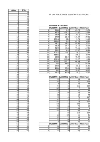
- 1. datos Bºrix 1 24 2 24 DE UNA POBLACION DE 200 DATOS SE SELECCIONA UNA MUESTR 3 24 4 26 5 26 6 27 7 27 NUMEROS ALEATORIOS 8 29 MUESTRA 1 MUESTRA2 MUESTRA3 MUESTRA4 9 30 1 79.01 3.17 65.79 25.76 10 31 2 45.39 119.77 51.07 119.39 11 33 3 28.56 38.16 83.6 44.79 12 34 4 94.09 36.48 116.32 109.01 13 35 5 105.42 18.2 7.76 24.13 14 36 6 119.69 2.61 82.76 39.35 15 36 7 24.23 94.47 48.96 24.05 16 36 8 58.26 14.74 18.12 48.09 17 38 9 71.71 43.62 75.15 117.36 18 38 10 63.21 4.93 27.97 90.85 19 40 11 102.15 111.7 18.1 112.96 20 41 12 118.93 48 108.6 29.78 21 41 13 53.58 66.73 79.49 62.96 22 44 14 109.96 113.86 59.27 8.84 23 47 15 105.07 105.11 64.99 27.82 24 51 16 2.54 66.07 117.31 107.13 25 51 17 27.69 105 66.3 85.21 26 51 18 25.84 37.22 50.06 28.86 27 51 19 91.3 46.81 10.97 80.17 28 51 20 79.11 80.86 34.1 55.11 29 51 30 52 MUESTRA 1 MUESTRA2 MUESTRA3 MUESTRA4 31 52 79 3 65 25 32 52 45 119 51 119 33 53 28 38 83 44 34 54 94 36 116 109 35 54 105 18 7 24 36 55 119 2 82 39 37 55 24 94 48 24 38 56 58 14 18 48 39 57 71 43 75 117 40 57 63 4 27 90 41 58 102 111 18 112 42 59 118 47 108 29 43 59 53 66 79 62 44 60 109 113 59 8 45 60 105 105 64 27 46 60 2 66 117 107 47 60 27 105 66 85 48 60 25 37 50 28 49 60 91 46 10 80 50 61 79 80 34 55 51 61 MUESTRA 1 MUESTRA2 MUESTRA3 MUESTRA4 52 61 1 64 24 63 51 53 62 2 60 65 61 65 54 62 3 51 56 64 60
- 2. 55 62 4 64 55 65 65 56 63 5 64 38 27 51 57 63 6 65 24 64 57 58 63 7 51 64 60 51 59 63 8 63 36 38 60 60 63 9 63 59 64 65 61 63 10 63 26 51 64 62 63 11 64 65 38 65 63 63 12 65 60 64 51 64 63 13 62 63 64 63 65 63 14 65 65 63 29 66 63 15 64 64 63 51 67 63 16 24 63 65 64 68 63 17 51 64 63 64 69 63 18 51 55 61 51 70 63 19 64 60 31 64 71 63 20 64 64 54 62 72 63 median 59.10 53.50 56.15 57.65 73 63 var. 95.88 220.37 151.92 80.13 74 63 desv. 9.79 14.84 12.33 8.95 75 64 76 64 77 64 TABLA DE RESUMEN POR AFIJACION PR 78 64 ESTRATO Ne ye We Se^2 79 64 1 20 59.10 0.071 95.88 80 64 2 20 53.50 0.071 220.37 81 64 2 20 56.15 0.071 151.92 82 64 4 20 57.65 0.071 80.13 83 64 5 20 54.60 0.071 217.31 84 64 totales 100 281.000 0.356 765.62 85 64 86 64 N 100 87 64 n 96 N * Z 2 * ∑We * Se 2 88 64 e 0.2 n= = 89 64 alfa 0.01 N * e 2 + 2 * ∑We * Se 2 Z 90 64 Z 2.58 91 64 92 64 calculode promedio por faij. Proporcional 93 64 94 64 95 64 1 96 97 64 64 ye = = N ∑ Ne * Ye 56.2000 98 64 99 64 100 64 1 101 102 64 64 calculo de la varianza del estimador ye = por faij. Proporcional = N ∑N 103 64 104 64 105 64 1 Se 2 106 107 64 64 V ( ye) = 2 * ∑ Ne( Ne ne) = 0.06 108 64 N ne 109 65
- 3. 110 65 111 65 calculo de la varianza del estimador por faij. Proporcional 112 65 113 65 114 65 S ( yes) = V ( y es) = 0.25 115 65 116 65 117 65 INTERVALO DE CONFIANZA 118 65 119 65 120 65 =e ± V ( yes ) = γ y t LI 55.55 Ls 56.85 FIJACION OPTIMA ESTRATO Ne ye We Se^2 1 20 59.10 0.071 95.884 2 20 53.50 0.071 220.368 2 20 56.15 0.071 151.92 4 20 57.65 0.071 80.13 5 20 54.60 0.071 217.31 totales 100 281.000 0.356 765.616 N 100 n 96 e 0.2 alfa 0.01 Z 2.58 calculo de la varianza del estimador por faij. Proporcional 1 Se 2 V ( ye ) = 2 * ∑ Ne ( Ne = ne) N ne calculo de la varianza del estimador por faij. Proporcional S ( ye s) = V ( y e s) = MUESTRA ASIGNACION IGUAL ESTRATO Ne ye We Se^2 1 20 59.10 0.0712 95.884 2 20 53.50 0.0712 220.368
- 4. 2 20 56.15 0.0712 151.92 4 20 57.65 0.0712 80.13 5 20 54.60 0.0712 217.31 totales 100 281 0.36 765.616 N 100 n 96.04 e 0.2 alfa 0.01 Z 2.58 calculode promedio por asisganacion igual 1 ye = = N ∑ Ne * Ye 56.2 calculode promedio por asisganacion igual 1 Se2 v = 2 ) = ∑ Ne(Ne ne) * = 0.06 N ne calculode promedio por asisganacion igual s ) == v = 0.24 calculode del intervalo de confianza 1 Se2 X ± Z ± 2 ∑ Ne(Ne ne) * ) = γ = N ne 56.2586 56.1414
- 5. ECCIONA UNA MUESTRA 100 Y DE DE TAMAÑO 50 MUESTRA5 88.38 5.59 38.58 110.09 74 58.54 116.14 88.75 61.22 59.77 41.04 6.47 47.51 105.79 76.16 15.67 3.25 101.33 19.77 69.95 MUESTRA5 88 5 38 110 73 58 116 88 61 59 41 6 47 105 76 15 3 101 19 69 MUESTRA5 64 26 56
- 6. 65 63 63 65 64 63 63 58 27 60 64 64 36 24 64 40 63 54.60 217.31 14.74 N e* S e ne=n* = ∑ N e* S e MEN POR AFIJACION PROPORCIONAL Se Ne-ye We*ye We*Se^2 ne Ne*Se^2 (Ne-ne) 9.79 1182 4.2 6.824 19 1917.68 1 14.84 1070 3.8 15.685 19 4407.37 1 12.33 1123 4.0 10.813 19 3038.47 1 8.95 1153 4.1 5.704 19 1602.68 1 14.74 1092 3.9 15.467 19 4346.11 1 60.66 5620 20.00 54.492 96 15312.316 4 We * Se 2 We * Se 2 ∑e e = = W * ye * α 1 ye = = N ∑ Ne * Ye
- 7. N e* S e ne=n* = CION OPTIMA ∑ N e* S e Se Ne-ye We*ye We*Se^2 ne Ne*Se^2 (Ne-ne) 9.792 1182.000 4.2 6.824 19 1917.68 1 14.845 1070.000 3.8 15.685 19 4407.37 1 12.33 1123.000 4.0 10.813 19 3038.47 1 8.95 1153.000 4.1 5.704 19 1602.68 1 14.74 1092.000 3.9 15.467 19 4346.11 1 60.656 5620.000 20.00 54.492 96 15312.316 4 0.0586 0.242 ASIGNACION IGUAL Se Ne-ye We*ye We*Se^2 ne Ne*Se^2 (Ne-ne) 9.792 1182 4.21 6.82 19 1917.68 1 14.845 1070 3.81 15.68 19 4407.37 0.8
- 8. 12.33 1123 4 10.81 19 3038.47 0.8 8.95 1153 4.1 5.7 19 1602.68 0.8 14.74 1092 3.89 15.47 19 4346.11 0.8 60.656 5620.000 20.000 54.492 96 15312.316 4.200
- 10. Ne(Ne-ne)Se^2/ne 79.90 183.64 126.60 66.78 181.09 638.01
- 11. Ne(Ne-ne)Se^2/ne Ne*Se 27.583 195.841 183.640 296.896 126.603 246.515 66.779 179.035 181.088 294.826 586 1213 Ne(Ne-ne)Se^2/ne Ne*Se 27.58 195.84 183.64 296.9
- 12. 126.6 246.51 66.78 179.04 181.09 294.83 586 1213
- 13. Nº.datos ºBrix 1 24 2 24 DE UNA POBLACION DE 200 DATOS SE SELECCIONA UNA MUEST 3 24 4 26 5 26 6 27 7 27 NUMEROS ALEATORIOS 8 29 MUESTRA 1 MUESTRA2 MUESTRA3 9 30 1 68.27 42.77 60.31 10 31 2 12.09 100.31 110.02 11 33 3 33.02 63.53 98.38 12 34 4 55.83 16.91 97.28 13 35 5 99.98 114.72 6.27 14 36 6 110.97 97.37 117.37 15 36 7 16.79 106.81 79.74 16 36 8 56.27 55.74 74.41 17 38 9 109.04 81.49 85.92 18 38 10 14.48 63.94 29.68 19 40 11 26.58 99.3 60.32 20 41 12 24 104.04 82.74 21 41 13 19.68 26.79 58.92 22 44 14 53.4 5.74 15.69 23 47 15 7.59 24.8 90.64 24 51 16 118.3 80.66 75.83 25 51 17 85.11 72.05 97.78 26 51 18 91.42 10.65 114.91 27 51 19 21.35 10.24 115.37 28 51 20 77.77 4.78 71.01 29 51 valores truncados 30 52 MUESTRA 1 MUESTRA2 MUESTRA3 31 52 68 42 60 32 52 12 100 110 33 53 33 63 98 34 54 55 16 97 35 54 99 114 6 36 55 110 97 117 37 55 16 106 79 38 56 56 55 74 39 57 109 81 85 40 57 14 63 29 41 58 26 99 60 42 59 23 104 82 43 59 19 26 58 44 60 53 5 15 45 60 7 24 90 46 60 118 80 75 47 60 85 72 97 48 60 91 10 114 49 60 21 10 115 50 61 77 4 71 51 61 MUESTRA 1 MUESTRA2 MUESTRA3 52 61 63 59 63 53 62 34 64 65 54 62 53 63 64
- 14. 55 62 62 36 64 56 63 64 65 27 57 63 65 64 65 58 63 36 64 64 59 63 63 62 63 60 63 65 64 64 61 63 36 63 51 62 63 51 64 63 63 63 47 64 64 64 63 40 51 63 65 63 62 26 36 66 63 27 51 64 67 63 65 64 64 68 63 64 63 64 69 63 64 31 65 70 63 41 31 65 71 63 64 26 63 72 63 median 53.30 53.75 60.05 73 63 var. 170.75 216.83 106.26 74 63 desv. 13.07 14.73 10.31 75 64 76 64 77 64 78 64 79 64 ∑X = 55.940 X == 80 64 K 279.70 81 82 64 64 X = 2 ∑ (X _ X )2 = 5 σ X == 83 64 7.83 K _1 84 64 X = 55.940 ((E73 - F80)^2 + (F σ2 X = 85 86 64 64 σ X = = ∑ (X _ X ) 2 = 87 64 K _1 2.8 σ 2 X = 7.83425 88 64 7.83425 89 64 σ X = = 90 64 4 91 64 σ X = =.7989 2 92 64 93 64 max 65 Li Ls 94 64 min 24 1 24 29.1744 95 64 rango 41 2 29.17 34.35 96 64 aintervalo(m) 8 3 34.35 39.52 97 64 amplitud ( C ) 5.174 4 39.52 44.70 98 64 alfa 1.96 5 44.70 49.87 99 64 6 49.87 55.05 100 64 7 55.05 60.22 101 64 8 60.22 65.39 102 64 totales 103 64 104 64 105 64 106 64 107 64 IC X z * 108 64 109 65
- 15. 110 65 Li 111 65 Ls 112 65 113 65 1 2 114 65 simple sistematico 115 65 promedio 55.94 47.5 116 65 varianza 7.83 4.88 117 65 desviacion 2.8 23.82 118 65 Ls 56.44 47.97 119 65 Li 55.44 47.02 120 65 si vale la pena aplicar este tratamiento
- 16. DATOS SE SELECCIONA UNA MUESTRA 100 Y DE DE TAMAÑO 50 EROS ALEATORIOS MUESTRA4 MUESTRA5 35.19 56.18 91.15 76.83 83.62 71.82 76.43 45.11 2.73 104.68 74.68 105.99 1.22 28.18 62.24 101.95 58.58 28.88 51.6 103.86 114.34 97.37 34.35 23.88 111.22 80.99 97.99 75.45 85.57 108.9 101.71 115.26 12.8 15.44 85.99 12.29 4.78 81.56 47.87 18.85 MUESTRA4 MUESTRA5 35 56 91 76 83 71 76 45 2 104 74 105 1 28 62 101 58 28 51 103 114 97 34 23 111 80 97 75 85 108 101 115 12 15 85 12 4 81 47 18 MUESTRA4 MUESTRA5 54 63 64 64 64 63
- 17. 64 60 24 64 63 64 24 51 63 64 63 51 61 64 65 64 54 47 65 64 64 64 64 64 64 65 34 36 64 34 26 64 60 38 55.20 57.40 222.38 112.36 14.91 10.60 median 279.70 55.94 sumdsuma var. 828.57 desv. 63.61 2 ∑ (X _ X )2 = σ X == K _1 ((E73 - F80)^2 + (F73 - F80)^2 + (G73 - F80)^2 + (H73 - F80)^2 + (I73 - F80)^2) σ2 X = 4 2 σ X = 7.83425 Xc f fa fr fra f*Xc 26.587 8 8 0.067 0.07 212.7 31.762 4 12 0.033 0.10 127.05 36.936 6 18 0.050 0.15 221.62 42.110 4 22 0.033 0.18 168.44 47.285 1 23 0.008 0.19 47.28 52.459 12 35 0.100 0.29 629.51 57.633 14 49 0.117 0.41 806.87 62.808 71 120 1 4459.35 357.580 120 0.41 6672.81 σ IC X z * n
- 18. 55.44 56.44 3 estratificadi conglomerado IC 56.2 58.26 0.06 1.54 si vale la pena aplicar este tratamiento 0.25 1.24 56.26 56.14 aplicar este tratamiento
- 19. 1 24 DE UNA POBLACION DE 200 DATOS SE SELECCIONA UNA MUESTR 2 24 3 24 4 26 5 26 6 27 NUMEROS ALEATORIOS 7 27 MUESTRA 1 MUESTRA2 MUESTRA3 8 29 1 68.86 16.21 117.52 9 30 2 35.85 8.58 56.43 10 31 3 6.45 24.44 3.46 11 33 4 76.75 116.87 103.72 12 34 5 10.11 33.93 44.82 13 35 6 13.42 39.92 74.23 14 36 7 63.35 75.44 10.24 15 36 8 48.79 36.54 77.09 16 36 9 30.07 82.35 103.89 17 38 10 20.83 17.06 63.18 18 38 11 35.58 1.7 58.47 19 40 12 115.03 44.92 42.67 20 41 13 34.45 53.77 39.94 21 41 14 35.06 52.78 89.21 22 44 15 29.21 98.51 99.58 23 47 16 52.62 83.09 38.95 24 51 17 65.75 47.9 2.98 25 51 18 89.32 10.33 19.4 26 51 19 24.55 105.83 26.27 27 51 20 19.51 36.65 104.51 28 51 78.17 39.63 19.99 29 51 valores truncados 30 52 68 16 117 31 52 35 8 56 32 52 6 24 3 33 53 76 116 103 34 54 10 33 44 35 54 13 39 74 36 55 63 75 10 37 55 48 36 77 38 56 30 82 103 39 57 20 17 63 40 57 35 1 58 41 58 115 44 42 42 59 34 53 39 43 59 35 52 89 44 60 29 98 99 45 60 52 83 38 46 60 65 47 2 47 60 89 10 19 48 60 24 105 26 49 60 19 36 104 50 61 valores buscados 51 61 1 63 36 65 52 61 2 54 29 63 53 62 3 27 51 24 54 62 4 64 65 64 55 62 5 31 53 60
- 20. 56 63 6 35 57 63 57 63 7 63 64 31 58 63 8 60 55 64 59 63 9 52 64 64 60 63 10 41 38 63 61 63 11 54 24 63 62 63 12 65 60 59 63 63 13 54 62 57 64 63 14 54 61 64 65 63 15 51 64 64 66 63 16 61 64 56 67 63 17 63 60 24 68 63 18 64 31 40 69 63 19 51 64 51 70 63 20 40 55 64 71 63 median 52.35 52.85 55.15 72 63 var. 136.87 180.77 190.87 73 63 desv. 11.70 13.44 13.82 74 63 75 64 MUESTREO SISTEMATICO 76 64 77 64 N 100 78 64 n 20 79 64 n ubicación de datos 80 64 1 2 47.1 81 64 2 7 46.3 82 64 3 12 40.8 83 64 4 17 53.30 84 64 5 22 45.9 85 64 6 27 45.5 86 64 7 32 42 87 64 8 37 47.1 88 64 9 42 47.7 89 64 10 47 45.8 90 64 11 52 54.5 91 64 12 57 40.3 92 64 13 62 54.8 93 64 14 67 45.9 94 64 15 72 40.2 95 64 16 77 56.3 96 64 17 82 45.2 97 64 18 87 53.1 98 64 19 92 50.4 99 64 20 97 47.7 100 64 promedio 47.5 101 64 var 23.82 102 64 desv. 4.88 103 64 z=95% 1.96 104 64 INTERVALOS DE CONFIANZA 105 64 106 64 s 107 64 I X z* ±_ γ = 108 64 n 109 65 110 65 li 47.02
- 21. 111 65 ls 47.97 112 65 113 65 114 65 115 65 116 65 117 65 118 65 119 65 120 65
- 23. OS SE SELECCIONA UNA MUESTRA 100 Y DE DE TAMAÑO 50 MUESTRA4 MUESTRA5 41.58 71.27 57.95 24.22 8.1 106.72 7.43 86.4 113.88 42.52 14.28 42.63 8.75 87.51 76.94 87.78 116.04 96.04 55.04 115.23 54.11 10.94 38.18 68.84 35.7 104.2 19.29 78.99 98.61 51.95 11.85 89.36 39.09 40.23 90.57 88.34 91.65 111.34 22.72 70.24 11.6 51.29 41 71 57 24 8 106 7 86 113 42 14 42 8 87 76 87 116 96 55 115 54 10 38 68 35 104 19 78 98 51 11 89 39 40 90 88 91 111 22 70 58 63 63 51 29 64 27 64 65 59
- 24. 36 59 29 64 64 64 65 64 62 65 62 31 56 63 54 64 40 64 64 61 33 64 57 57 64 64 64 65 44 63 51.80 60.65 201.22 60.34 14.19 7.77 MUESTREO SISTEMATICO Intervalos N 5 I == n
- 27. 1 24 2 24 DE UNA POBLACION DE 200 DATOS SE SELECCIONA UNA MUESTR 3 24 4 26 5 26 6 27 7 27 NUMEROS ALEATORIOS 8 29 MUESTRA 1 MUESTRA2 MUESTRA3 MUESTRA4 9 30 1 77.95 8.55 35.85 118.88 10 31 2 34.45 51.9 91.94 34.83 11 33 3 55.88 47.02 94 104.89 12 34 4 4.56 20.48 27.53 8.76 13 35 5 68 13.33 36.54 14.3 14 36 6 101.07 10.82 86.8 105.61 15 36 7 43.68 75.13 95.79 16.16 16 36 8 51.19 92.82 21.93 59.95 17 38 9 43.05 93.56 35.6 77.26 18 38 10 62.24 115.94 97.65 2.97 19 40 11 16.43 96.37 25.09 100.7 20 41 12 99.25 71.31 64.58 30.51 21 41 13 55.78 96.63 58.12 43.08 22 44 14 17.77 4.24 35.94 14.87 23 47 15 52.91 43.92 109.35 11.63 24 51 16 30.34 119.68 60.1 30.4 25 51 17 8.05 14.63 23.29 51.3 26 51 18 25.59 78.83 115.06 52.57 27 51 19 56.49 17.34 85.32 16.02 28 51 20 39.72 19.43 97.66 3.73 29 51 30 52 valores truncados 31 52 77 8 35 118 32 52 34 51 91 34 33 53 55 47 93 104 34 54 4 20 27 8 35 54 67 13 36 14 36 55 101 10 86 105 37 55 43 75 95 16 38 56 51 92 21 59 39 57 43 93 35 77 40 57 62 115 97 2 41 58 16 96 25 100 42 59 99 71 64 30 43 59 55 96 58 43 44 60 17 4 35 14 45 60 52 43 109 11 46 60 30 119 60 30 47 60 8 14 23 51 48 60 25 78 115 52 49 60 56 17 85 16 50 61 39 19 97 3 51 61 52 61 MUESTREO POR CONGLOMERADO
- 28. 53 62 54 62 valores buscados 55 62 C1 C2 C3 C4 56 63 64 29 54 65 57 63 54 61 64 54 58 63 62 60 64 64 59 63 26 41 51 29 60 63 63 35 55 36 61 63 64 31 64 64 62 63 59 64 64 36 63 63 61 64 41 63 64 63 59 64 54 64 65 63 63 65 64 24 66 63 36 64 51 64 67 63 64 63 63 52 68 63 62 64 63 59 69 63 38 26 54 36 70 63 61 59 65 33 71 63 52 65 63 52 72 63 29 36 47 61 73 63 51 64 65 61 74 63 63 38 64 36 75 64 57 40 64 24 76 64 yi 1088 1033 1174 977 77 64 Pro.yi 54.40 51.65 58.70 48.85 78 64 SUMAyi 269.60 79 64 80 64 N 20 81 64 n 100 82 64 M 10 83 64 m 5 84 64 85 64 CALCULO DE LA VARIANZA DEL ESTIMADOR 86 64 87 64 ( Y j) 88 64 Y.. = 53.92 m 89 64 90 64 91 64 CALCULO DE LA VARIANZA DEL ESTIMADOR 92 64 93 64 2 58.26 64 ( j Y - y..) 94 95 64 96 64 CALCULO DE LA VARIANZA ENTRE CONGLOMERADOS 97 64 98 64 99 64 2 N * ∑ (yj - y..) 2 100 64 SE = 101 64 m -1 102 64 103 64 2 * 5 .2 0 8 6 104 64 SE 2 = 291.32 5 -1 SE 2 = 2 1 .3 9
- 29. 2 * 5 .2 0 8 6 SE 2 = 105 64 5 -1 106 64 SE 2 = 2 1 .3 9 107 64 108 64 109 65 CALCULO DE LA VARIANZA DENTRO DE CONGLOMERADOS 110 65 111 65 2 ∑∑ (yij - y j ) 2 112 65 SD = 113 65 M(N - 1) 114 65 115 65 C1 C2 C3 C4 116 65 1 92.16 513.02 22.09 260.82 117 65 2 0.16 87.42 28.09 26.52 118 65 3 57.76 69.72 28.09 229.52 119 65 4 806.56 113.42 59.29 394.02 120 65 5 73.96 277.22 13.69 165.12 6 92.16 426.42 28.09 229.52 7 21.16 152.52 28.09 165.12 8 43.56 152.52 313.29 200.22 9 21.16 152.52 22.09 229.52 10 73.96 178.22 28.09 617.52 11 338.56 152.52 59.29 229.52 12 92.16 128.82 18.49 9.92 13 57.76 152.52 18.49 103.02 14 268.96 657.92 22.09 165.12 15 43.56 54.02 39.69 251.22 16 5.76 178.22 18.49 9.92 17 645.16 244.92 136.89 147.62 18 11.56 152.52 39.69 147.62 19 73.96 186.32 28.09 165.12 20 6.76 135.72 28.09 617.52 TOTALES 2827 4167 980 4365 SUMA.SUM. 178 46 SD 2 = 14.9173 1( 0 010 -1) SD 2 = 1. 12 4 7 9 CALCULO DE LA VARIANZA TOTAL. 2 (M 1) SE 2 + 8 N 1) SD 2 M ST = (N * M) - 1 (10 1)291 .315 > + +MAS + (20 1)14 .9173 10 ST 2 = (20 * 10) - 1 5456.122 27.42 ST 2 = 199 2 ST = 27.4176
- 30. (20 * 10) - 1 5456.122 ST 2 = 199 ST 2 = 27.4176 CALCULO DE LA VARIANZA DEL ESTIMADOR 1 [ M − _ m] [ M ( N _ 1)] V (y..)= *( )* 2 * SE 2 m M N ( M _ 1) 1 [10 _ 5] [10(20 _ 1)] V (y..)= * ( )* 2 * 291.315 5 10 20 (10 _ 1) V (y..)= 0.2* 0.5* 0.05277 291.315 * V (y..)= 1.53727 1.54 1.24
- 31. ECCIONA UNA MUESTRA 100 Y DE DE TAMAÑO 50 MUESTRA5 91.78 7.99 108.08 92.97 52.27 23.98 99.25 91.21 82.1 77.62 78.82 23.73 55.9 11.43 21.59 29.57 42.32 44.04 39.82 58.17 91 7 108 92 52 23 99 91 82 77 78 23 55 11 21 29 42 44 39 58
- 32. C5 64 27 64 64 61 47 64 64 64 64 64 47 62 33 41 51 59 60 57 63 1120 56.00
- 33. C5 64 841 64 64 25 81 64 64 64 64 64 81 36 529 225 25 9 16 1 49 2430 14768