Ejemplos problemas resueltos de estadística

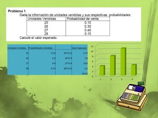
1. 0
2
4
6
8
10
12
1 2 3 4
Unidades Vendidas Probabilidades Vendidas Valor Esperado
25 0.15 25*0.15 3.75
26 0.3 26*0.3 7.8
27 0.4 27*0.4 10.8
28 0.15 28*0.15 4.2
26.55

2. Juego Premio P.E.
Valor
Esperado
Ganar 50,000 0.550000*0.5 25000
Perder 50,000 0.550000*0.5 25000
50000
0
5000
10000
15000
20000
25000
1 2

3. Cantidad Tipo de premio Valor del premio Probabilidad Valor esperado
1 mayor 1000
0.000000667
0 1000*0.000000667 0.000667
2 secos 50
0.000000667
0 50*0.000000667 0.00003335
2 secos 20
0.000000667
0 20*0.000000667 0.00001334
100 secos 2
0.000000667
0 2*0.000000667 0.000001334
149 Secos 0.5
0.000099333
0 0.5*0.000099333 0.000049666
0.00076469
0
0.0001
0.0002
0.0003
0.0004
0.0005
0.0006
0.0007
1 2 3 4 5

4. 9
9.5
10
10.5
11
11.5
12
1 2 3

5. Alternativa S1 Probabilidad S2 Probabilidad S3 Probabilidad Valor Esperado
A1 $50 0.30 $70 0.50 $100 0.20 70
A2 $90 0.30 $40 0.50 $80 0.20 63
A3 $70 0.30 $60 0.50 $90 0.20 69
202
58
60
62
64
66
68
70
1 2 3

7. P=0.0001
N=20000
Binomial with n = 20000 and p = 0.0001
x P( X <= x )
2 0.676676 = 0.323324

8. A) Binomial with n = 20 and p = 0.2
x P( X <= x )
2 0.206085
B) Binomial with n = 20 and p = 0.2
x P( X = x )
4 0.218199
C) Binomial with n = 20 and p = 0.2
x P( X <= x )
3 0.411449

9. A) Binomial with n = 12 and p = 0.1 x P( X = x ) 2 0.230128
B) Binomial with n = 12 and p = 0.1x P( X <= x ) 1 0.659002
C) Binomial with n = 20 and p = 0.1x P( X <= x ) 0 0.121577

10. A) Binomial with n = 2 and p = 0.03
x P( X = x )
0 0.9409
B) Binomial with n = 2 and p = 0.03
x P( X = x )
1 0.0582
C) Binomial with n = 2 and p = 0.03
x P( X = x )
2 0.0009

12. media=5
P(x<3)=p(0)+p(1)+p(2)
Cumulative Distribution Function
Poisson with mean = 5
x P( X <= x )
2 0.124652

13. media=5
P(x>10)=1-[ p(0)+p(1)+p(2)+…+p(10)]
Cumulative Distribution Function
Poisson with mean = 5
x P( X <= x )
10 0.986305
1 – 0.986305 = .013695

14. p=.001
n= 3000
a) media= np =(.001)(3)=.003
b) P(x=0)
Probability Density Function
Poisson with mean = 3
x P( X = x )
0 0.0497871

15. Media=2000
ℓ=200
P(2000≤ x ≤ 2400)
Cumulative Distribution Function
Normal with mean = 2000 and standard deviation = 200
x P( X <= x )
2000 0.5
Cumulative Distribution Function
Normal with mean = 2000 and standard deviation = 200
x P( X <= x )
2400 0.977250
0.977250 – 0.5 = 0.47725

16. Media=13 cm
σ=0.1
P(13≤ x ≤ 13.2)
Cumulative Distribution Function
Normal with mean = 13 and standard deviation = 0.1
x P( X <= x )
13 0.5
Cumulative Distribution Function
Normal with mean = 13 and standard deviation = 0.1
x P( X <= x )
13.2 0.977250
0.977250 – 0.5 = 0.47725

17. Media=980
ℓ=48
a) P(x≥1000)
b)P(x≤940)
c)P(960 ≤ x ≤ 1060)
a) Cumulative Distribution Function
Normal with mean = 980 and standard deviation = 40
x P( X <= x )
1000 0.691462 1-0.691462=0.308538
b) Cumulative Distribution Function
Normal with mean = 980 and standard deviation = 40
x P( X <= x )
940 0.158655
c) Cumulative Distribution Function
Normal with mean = 980 and standard deviation = 40
x P( X <= x )
960 0.308538
Cumulative Distribution Function
Normal with mean = 980 and standard deviation = 40
x P( X <= x )
1060 0.977250
0.977250 – 0.308538= 0.668712

18. Media=5.10
ℓ=0.40
a) P(x≥5.4)
b)P(4.70 ≤ x ≤5.4)
c)P(x ≥3.40)
a) Cumulative Distribution Function
Normal with mean = 5.1 and standard deviation = 0.4
x P( X <= x )
5.4 0.773373
b) Cumulative Distribution Function
Normal with mean = 5.1 and standard deviation = 0.4
x P( X <= x )
4.7 0.158655 0.773373 - 0.158655 =0.614718
c) Cumulative Distribution Function
Normal with mean = 5.1 and standard deviation = 0.4
x P( X <= x )
3.9 0.0013499
1 – 0.0013499 = 0.9987

19. N=1500
n=300
p=300/1500
= 0.2
q=1-0.2= 0.8
Nievl de Confianza= 0.99
α= 1 -0.99 = .01
z= -2.5758293
0.22660305* 1500= 339.904576LS
0.17339695* 1500= 260.095424LI
a)
b) 0.21032796*1500= 315.491933LS
0.18967204*1500= 284.508067LI
Cota del error [284.50, 315.49]

20. N1=100 N2=100
Media=1425 Media=1905
σ=40 σ=30
Cota del error 2.83666003
1.16333997

21. N=2500
n=85
p=0.65
q=1-0.65=0.35
Nievl de Confianza= 0.97 Nivel de Confianza= 0.85
α= 1 -0.97 = 0.03 α= 1 -0.97 = 0.15
z= -2.17009038 z= -1.43953147
0.67070134* 85= 57.0096141LS 0.663732255*85= 56.4172417LS
0.62327468* 85= 52.9783479LI 0.632271735*85= 53.7430975LI

22. M=5.3
σ=1.2
n=26 5.783327959 LS
Nievl de Confianza= 96% 4.816672041 LI
α=0.04
z= -2.05374891 Verdadera Media= 5

24. H0= m1=m2
HA: m1≠m2
One-Sample T
Test of mu = 55 vs not = 55
N Mean StDev SE Mean 99% CI T
P
17 50.00 7.00 1.70 (45.04, 54.96) -2.95
0.010
Inverse Cumulative Distribution Function
Student's t distribution with 16 DF
P( X <= x ) x
0.01 -2.58349
Rechazamos H0 por que la T calculada es > que la de tablas
Afirmamos con el 99% de probabilidades que no es posible que la media de la población
sea 55.

25. H0= m1 = m2
H4: m1≠m2
G1= n1+n2-2
=8+14-2=20
Two-Sample T-Test and CI
Sample N Mean StDev SE Mean
1 8 50.00 5.00 1.8
2 14 45.00 4.00 1.1
Difference = mu (1) - mu (2)
Estimate for difference: 5.00
95% CI for difference: (0.50, 9.50)
T-Test of difference = 0 (vs not =): T-Value = 2.42 P-Value =
0.032 DF = 12
Inverse Cumulative Distribution Function
Student's t distribution with 20 DF
P( X <= x ) x
0.05 -1.72472
T> que la t de tabla, se rechaza Ho
Por lo tanto si existe una diferencia
significativa entre las medias

26. t= (σ₁²-σ₂²) √n-2 1.60416667
2σ₁σ₂√1-r₁₂²
Inverse Cumulative Distribution Function
Student's t distribution with 49 DF
P( X <= x ) x
0.01 -2.40489
Se acepta H0 por que la t de tablas es mayor que la calculada

27. Two-Sample T-Test and CI: Campaña 1, Campaña 2
Two-sample T for Campaña 1 vs Campaña 2
N Mean StDev SE Mean
Campaña 1 6 20.17 5.98 2.4
Campaña 2 6 22.17 7.25 3.0
Difference = mu (Campaña 1) - mu (Campaña 2)
Estimate for difference: -2.00
99% CI for difference: (-14.47, 10.47)
T-Test of difference = 0 (vs not =): T-Value = -0.52 P-Value =
0.615 DF = 9
Inverse Cumulative Distribution Function
Student's t distribution with 10 DF
P( X <= x ) x
0.01 -2.76377
H0: m1≠m2
H1: m1≠m2
Aceptamos Ho

28. Inverse Cumulative Distribution Function
Student's t distribution with 18 DF
P( X <= x ) x
0.05 -1.73406
√1 - r² 0.189
n-2
0.6±1.73(.189)= 0.6±0.3 = [.91, .23]
La variabilidad del coeficiente esta entre 0.91 y 0.27

29. H0; r1=r2
Hq; r1≠r2
n= 50
r1= 0.72 -0.24 -0.520307601
r2= 0.78 0.611751584
r= 0.6 -0.850521053
Inverse Cumulative Distribution Function
Student's t distribution with 47 DF
P( X <= x ) x
0.05 -1.67793
t
T calculada es < t de tablas; por tanto aceptamos H0