La curva de crecimiento del ganado tiene una forma sigmoidea que puede ser ajustada con modelos de regresión aleatoria. El objetivo de este estudio fue ajustar un modelo de regresión aleatoria con base en polinomios de Legendre, y estimar componentes de varianza y parámetros genéticos, para datos de crecimiento en bovinos Tropicarne. Se analizó la información de 12 890 pesadas mensuales, del nacimiento a los 24 meses de edad de 1787 becerros. El pedigrí incluyó 2504 animales. Se compararon 27 modelos lineales, cuadráticos y cúbicos para ajuste de los efectos genéticos (EGA) y de ambiente permanente (APA) del animal, con tres estructuras en las varianzas de residuales (homogénea, y heterogénea de seis y doce clases). Una vez seleccionado el modelo con los efectos del animal, se analizaron otros nueve modelos para determinar la posible adición de los efectos maternos, genéticos (EGM) y de ambiente permanente (APM). Los análisis se realizaron con el programa DFREML. Los modelos se compararon con base en: proporción de verosimilitudes, criterio de información de Akaike y criterio de información bayesiana. El modelo con mejor ajuste incluyó los EGA de orden cuadrático y los efectos de APA, EGM y APM de orden cúbico, con varianza residual heterogénea en doce clases. Las varianzas fenotípicas de EGA y de EGM presentaron tendencia positiva con la edad; sin embargo, la varianza residual presentó un comportamiento cuadrático en los primeros ocho meses del crecimiento y luego se mantuvo constante. La heredabilidad directa promedio fue 0.079, con valores de 0.006 a 0.06 hasta los siete meses; y desde los ocho meses fue constante (alrededor de 0.11). La heredabilidad materna promedio fue 0.084, con valores de 0.02 a 0.06 hasta los siete meses y de 0.07 a 0.16 desde de los ocho meses de edad. El modelo de regresión aleatoria fue el mejor desde los nueve meses de edad, pero subestimó los parámetros genéticos para edades menores.

1. AJUSTE DE MODELOS DE REGRESIÓN ALEATORIA EN EVALUACIONES
GENÉTICAS DE BOVINOS TROPICARNE
ADJUSTMENT OF RANDOM REGRESSION MODELS ON GENETIC
EVALUATIONS OF TROPICARNE CATTLE
Joel Domínguez-Viveros1*, Felipe A. Rodríguez-Almeida1, Rafael Nuñez-Domínguez2, Juan Á. Ortega-Gutiérrez1,
Rodolfo Ramírez-Valverde2, Eduardo Santellano-Estrada1, José L. Espinosa-Villavicencio3
1
Facultad de Zootecnia y Ecología, Universidad Autónoma de Chihuahua. 31031. Periférico
Francisco R. Almada, km 1. Chihuahua, México. (jodominguez@uach.mx). 2Departamen-
to de Zootecnia, Universidad Autónoma Chapingo. 56230. Chapingo, Estado de México.
3
Universidad Autónoma de Baja California.
Resumen Abstract
La curva de crecimiento del ganado tiene una forma sig- The growth curve of cattle has a sigmoid shape that can be
moidea que puede ser ajustada con modelos de regresión adjusted with random regression models. The objective of
aleatoria. El objetivo de este estudio fue ajustar un modelo this study was to adjust a random regression model based
de regresión aleatoria con base en polinomios de Legendre, on Legendre polynomials and to estimate components
y estimar componentes de varianza y parámetros genéticos, of variance and genetic parameters for data on growth
para datos de crecimiento en bovinos Tropicarne. Se analizó of Tropicarne cattle. Information from 12 890 monthly
la información de 12 890 pesadas mensuales, del nacimiento weighings of 1787 calves, from birth to 24 months old, was
a los 24 meses de edad de 1787 becerros. El pedigrí incluyó analyzed. The pedigree included 2504 animals. Twenty-
2504 animales. Se compararon 27 modelos lineales, cuadrá- seven linear, quadratic and cubic models were compared
ticos y cúbicos para ajuste de los efectos genéticos (EGA) y for adjustment of the genetic (EGA) and animal permanent
de ambiente permanente (APA) del animal, con tres estruc- environmental (APA) effects, with three structures in residuals
turas en las varianzas de residuales (homogénea, y hetero- variances (homogeneous and heterogeneous of six and
génea de seis y doce clases). Una vez seleccionado el modelo twelve classes). Once the model was selected with the animal
con los efectos del animal, se analizaron otros nueve mo- effects, another nine models were analyzed to determine the
delos para determinar la posible adición de los efectos ma- possible addition of maternal genetic (EGM) and permanent
ternos, genéticos (EGM) y de ambiente permanente (APM). environmental (APM) effects. The analyses were performed
Los análisis se realizaron con el programa DFREML. Los with the DFREML software. Models were compared based
modelos se compararon con base en: proporción de vero- on the likelihood ratio test, Akaike’s information criterion,
similitudes, criterio de información de Akaike y criterio de and the Bayesian information criterion. The model with the
información bayesiana. El modelo con mejor ajuste incluyó best fit included the quadratic order EGA and the effects of
los EGA de orden cuadrático y los efectos de APA, EGM APA, EGM and APM of cubic order, with heterogeneous
y APM de orden cúbico, con varianza residual heterogénea residual variance in twelve classes. The phenotypic variances,
en doce clases. Las varianzas fenotípicas de EGA y de EGM EGA and EGM, showed a positive trend on age; however, the
presentaron tendencia positiva con la edad; sin embargo, residual variance showed quadratic behavior in the first eight
la varianza residual presentó un comportamiento cuadráti- months of growth after which it remained constant. Average
co en los primeros ocho meses del crecimiento y luego se direct heritability was 0.079 with values of 0.006 to 0.06 up
mantuvo constante. La heredabilidad directa promedio fue to seven months of age; as of eight months it was constant,
0.079, con valores de 0.006 a 0.06 hasta los siete meses; y around 0.11. Average maternal heritability was 0.084, with
desde los ocho meses fue constante (alrededor de 0.11). La values of 0.02 to 0.06 up to seven months and 0.07 to 0.16
heredabilidad materna promedio fue 0.084, con valores de as of eight months of age. The random regression model was
well fitted as of nine months of age, but it underestimated the
genetic parameters for younger ages.
*Autor responsable v Author for correspondence.
Recibido: Marzo, 2010. Aprobado: Enero, 2011.
Publicado como ARTÍCULO en Agrociencia 45: 325-337. 2011. Key words: cattle, genetic improvement, genetic parameters.
325

2. AGROCIENCIA, 1 de abril - 15 de mayo, 2011
0.02 a 0.06 hasta los siete meses y de 0.07 a 0.16 desde de Introduction
los ocho meses de edad. El modelo de regresión aleatoria fue
G
el mejor desde los nueve meses de edad, pero subestimó los enetic evaluations of growth traits of beef
parámetros genéticos para edades menores. cattle are traditionally based on the analysis
of weights adjusted to determined ages
Palabras clave: ganado, mejoramiento genético, parámetros using the animal model with maternal effects and,
genéticos. in certain cases, multivariate models (Rosales et al.,
2004; Ríos, 2008; Domínguez-Viveros et al., 2009).
Introducción However, this type of analysis does not consider
that growth of beef cattle is adjusted to a sigmoid
L
as evaluaciones genéticas de características curve, with changes resulting from genetic and
del crecimiento de bovinos para carne se ba- environmental effects (Lawrence and Fowler, 2002).
san tradicionalmente en el análisis de pesos The analysis of weights adjusted to determined ages
ajustados a determinadas edades, mediante el mo- assumes that all of the animals have a similar growth
delo animal con efectos maternos y en ciertos ca- curve and that the genetic and environmental effects
sos multivariados (Rosales et al., 2004; Ríos, 2008; and the variances and covariances of the random
Domínguez-Viveros et al., 2009). Sin embargo, este effects are constant within the adjusted interval,
tipo de análisis no considera que el crecimiento de regardless of possible genetic differences among the
los bovinos para carne se ajusta a una curva sigmoi- animals (Meyer, 1998a). The growth curve of the
dea, con cambios producto de los efectos genéticos animals is usually obtained with weights at different
y ambientales (Lawrence y Fowler, 2002). El análi- ages, considered longitudinal data or repeated
sis de pesos ajustados a determinadas edades supo- measurements of the same trait.
ne que todos los animales presentan curva similar Repeated measurements have been analyzed with
de crecimiento y que los efectos genéticos y am- three types of models: 1) repeatability (Henderson,
bientales y las varianzas y covarianzas de los efectos 1984); 2) multivariate or multiple trait (Ramírez-
aleatorios son constantes en el intervalo ajustado, Valverde et al., 2007); 3) random regression
sin considerar posibles diferencias genéticas entre (Albuquerque and Meyer, 2001; Meyer, 2001). The
animales (Meyer, 1998a). La curva de crecimiento random regression models (MRA) better define
de los animales usualmente se obtiene con los pesos random effects since they use data and information
de diferentes edades, considerados datos longitudi- directly from each animal without transformations
nales o medida repetida de la misma característica. or arbitrary adjustments (Sakaguti, 2003) and
Las medidas repetidas se han analizado con tres assumptions on the shape of the growth curve or
tipos de modelos: 1) repetibilidad (Henderson, variance and covariance structure (Meyer, 1998a).
1984); 2) multivariados o multicaracteres (Ramí- In the same way, with MRA, a trajectory is adjusted
rez-Valverde et al., 2007); 3) de regresión aleatoria for each individual as a deviation from the average
(Albuquerque y Meyer, 2001; Meyer, 2001). Los growth curve of a population (Meyer, 2000), and it
modelos de regresión aleatoria (MRA) definen me- is possible to predict genetic values for each point
jor los efectos aleatorios, ya que usan directamente on the growth curve (Albuquerque and Meyer, 2001;
los datos e información de cada animal, sin trans- Nobre et al., 2003a).
formaciones o ajustes arbitrarios (Sakaguti, 2003) y Tropicarne is the first synthetic beef cattle breed
supuestos sobre la forma de la curva de crecimiento developed in México. The characteristics of the race
o la estructura de varianzas y covarianzas (Meyer, and of the production systems have been described
1998a). Del mismo modo, con los MRA se ajusta by Domínguez-Viveros et al. (2003) and Ruíz-Flores
una trayectoria para cada individuo, como una des- et al. (2006). Genetic evaluations of Tropicarne
viación de la curva de crecimiento promedio de la cattle growth began with analysis of weight at birth,
población (Meyer, 2000) y es posible predecir valo- weaning, and 18 months of age, with univariate
res genéticos para cada punto de la curva de creci- and multivariate models (Domínguez-Viveros et al.,
miento (Albuquerque y Meyer, 2001; Nobre et al., 2003; Ramírez-Valverde et al., 2007). The objectives
2003a). of the present study were to adjust random regression
326 VOLUMEN 45, NÚMERO 3

3. AJUSTE DE MODELOS DE REGRESIÓN ALEATORIA EN EVALUACIONES GENÉTICAS DE BOVINOS TROPICARNE
Tropicarne es la primera raza sintética de bovinos models in the genetic evaluation of Tropicarne
para carne desarrollada en México. Las caracterís- beef cattle growth and to estimate the (co)variance
ticas de la raza y de los sistemas de producción han components and genetic parameters for the growth
sido descritos por Domínguez-Viveros et al. (2003) period evaluated. The genetic evaluations based on
y Ruíz-Flores et al. (2006). En bovinos Tropicarne, the adjustment of random regression models will
las evaluaciones genéticas del crecimiento se iniciaron increase the precision of animal selection criteria
con el análisis del peso en el nacimiento, destete y a through adjustments of the growth curve.
los 18 meses de edad, con modelos univariados y mul-
tivariados (Domínguez-Viveros et al., 2003; Ramírez- Materials and Methods
Valverde et al., 2007). Los objetivos del presente es-
tudio fueron ajustar modelos de regresión aleatoria Genealogical information and growth records of Mexican
en la evaluación genética del crecimiento en bovinos Tropicarne cattle were analyzed. The pedigree file included 2504
Tropicarne y estimar los componentes de (co)varianza animals born in the period 1973 to 2004. The growth database
y parámetros genéticos para el periodo de crecimiento included 12 890 monthly weighings from birth up to 24 months
evaluado. Las evaluaciones genéticas con base en el of age of 1787 animals born between 1990 and 2004 (Table 1).
ajuste de modelos de regresión aleatoria, incrementa-
rán la precisión de los criterios para seleccionar ani- Models and analyses performed
males mediante ajustes de la curva de crecimiento.
To describe growth, the random regression model was used
Materiales y Métodos based on Legendre orthogonal polynomials (Kirkpatrick et al.,
1990; Schaeffer, 2004):
Se analizó la información genealógica y registros de creci-
miento de bovinos Tropicarne en México. El archivo de pedigrí k=4 ka−1 kc−1
yij = Fij + ∑ βr Φr ( aij ) + ∑ αir Φir ( aij ) + ∑ ρir Φir ( aij )
incluyó 2504 animales nacidos de 1973 a 2004; la base de datos
r=2 r=2
de crecimiento incluyó 12 890 pesadas mensuales, desde el na- km−1 kq−1
cimiento hasta los 24 meses de edad, de 1787 bovinos nacidos + ∑ γir Φir ( aij ) + ∑ δir Φir ( aij ) + εij
r=2 r=2
entre 1990 y 2004 (Cuadro 1).
Modelos y análisis realizados where yij is the jth weight of the ith animal; Fij is the set of fixed
effects in the jth register of the ith animal, which considers
Para describir el crecimiento se utilizó el modelo de regre- contemporaneous groups (defined by the combination of year-
sión aleatoria, con base en polinomios ortogonales, de Legendre time of weighing, sex and age of the animal in months; the
(Kirkpatrick et al., 1990; Schaeffer, 2004): number of contemporaneous groups by age is presented in Table
Cuadro 1. Medias ( y ) y desviaciones estándar (s) de peso (kg) al nacer (PN), edades (meses; edd), número de observaciones (n)
y grupos contemporáneos (gc) analizados en la base de datos de bovinos Tropicarne.
Table 1. Means ( y ) and standard deviations (s) for weight (kg) at birth (PN), ages (months; edd), number of observations (n)
and contemporaneous groups (gc), analyzed on the database of Tropicarne cattle.
edd n(gc) y s edd n(gc) y s edd n(gc) y s
PN§ 1767(80) 34.31.76 9 699(53) 218.237.5 17 594(49) 313.453.7
1 60(8) 67.014.2 10 573(44) 236.740.8 18 662(54) 323.156.8
2 37(7) 82.310.1 11 659(56) 242.641.9 19 633(60) 333.960.2
3 13(3) 96.813.8 12 813(59) 250.338.6 20 594(54) 338.060.5
4 15(3) 134.122.6 13 841(62) 257.343.5 21 451(38) 348.664.1
5 47(7) 152.325.6 14 722(54) 269.745.7 22 327(37) 365.767.8
6 105(14) 169.328.3 15 654(49) 286.250.5 23 325(44) 374.668.8
7 372(34) 189.335.5 16 578(41) 304.953.2 24 325(42) 371.964.7
8 1024(65) 208.833.0
DOMÍNGUEZ-VIVEROS et al. 327

4. AGROCIENCIA, 1 de abril - 15 de mayo, 2011
k=4 ka−1 kc−1 1) and the covariable age of the cow, with linear and quadratic
yij = Fij + ∑ βr Φr ( aij ) + ∑ αir Φir ( aij ) + ∑ ρir Φir ( aij ) effects; aij is the jth standardized age (1 a 1) at which the ith
r=2 r=2
km−1 kq−1 animal was weighed; ir is the rth Lengendre polynomial; k is the
+ ∑ γir Φir ( aij ) + ∑ δir Φir ( aij ) + εij order of the evaluated polynomials (2  linear, 3  quadratic,
r=2 r=2 and 4  cubic), in which ka  direct genetic effects, kc 
animal permanent environmental effects, km  maternal genetic
donde, yij es el j-ésimo peso del i-ésimo animal; Fij es el con- effects, and kq  permanent maternal environmental effects; r
junto de efectos fijos en el j-ésimo registro del i-ésimo animal, is the coefficient of regression of cubic order for modeling the
que considera los grupos contemporáneos (definidos por la population mean; ir and ir are the coefficients of regression
combinación de año-época de pesada, sexo y edad del animal for modeling the direct random, genetic and permanent
en meses; el número de grupos contemporáneos por edad se environmental effects, of the rth polynomial for the ith animal;
presenta en el Cuadro 1) y la covariable edad de la vaca, con ir and ir are the coefficients of regression for modeling the
efectos lineal y cuadrático; aij es la j-ésima edad estandarizada maternal random, genetic, and permanent environmental effects
(1 a 1) a la que se pesó el i-ésimo animal, ir es el r-ésimo of the rth polynomial for the ith animal; and ij is the residual
polinomio de Legendre; k es el orden de los polinomios eva- effect. The cubic order for modeling the population mean ()
luados (2  lineal, 3  cuadrático y 4  cúbico), en el que was defined in preliminary analyses considering only fixed effects
ka  efectos genéticos directos, kc  efectos de ambiente per- of year and time of birth and sex of the animal as classes, plus
manente del animal, km  efectos genéticos maternos y kq  the covariable animal age in linear, quadratic and cubic function.
efectos maternos de ambiente permanente; r es el coeficiente
de regresión de orden cúbico para modelar la media de la po- The matrix form of the above complete model, with its
blación, ir y ir son los coeficientes de regresión para modelar respective assumptions, is the following: y  Xb  Z1a  Z2c
los efectos aleatorios directos, genéticos y del ambiente per-  Z3m  Z4q  e; E[y]  Xb; E[a]  E[c]  E[m]  E[q] 
manente, del r-ésimo polinomio para el i-ésimo animal; ir y E[e]  0. Var(a)  ka  A; Var(c)  kc  INd ; Var(m)  km 
ir, son los coeficientes de regresión para modelar los efectos A; Var(q)  kq  INm; Var(e)  R
aleatorios maternos, genéticos y de ambiente permanente del
r-ésimo polinomio para el i-ésimo animal; y ij , es el efecto where y is the vector of n observations (referring to the number
residual. El orden cúbico para modelar la media de la pobla- of animals with productive records, Nd); b is the vector of
ción () se definió en análisis preliminares considerando sólo fixed effects of contemporaneous groups and coefficients
efectos fijos de año y época de nacimiento y sexo del animal of regression of first, second and third order of the effect of
como clases, más la covariable edad del animal en función li- age; a is a vector, ka  ND random regression coefficients for
neal, cuadrática y cúbica. additive direct genetic effects, where ND denotes the total
number of animals in the genetic relationships matrix, with
La forma matricial del modelo anterior completo, con sus res- and without weight records; c is a vector, kc  Nd random
pectivas suposiciones es: y  Xb  Z1a  Z2c  Z3m  Z4q  e; regression coefficients for animal permanent environmental
E[y]  Xb; E[a]  E[c]  E[m]  E[q]  E[e]  0. Var(a)  ka effects; m is a vector, km  ND random regression coefficients
 A; Var(c)  kc  INd ; Var(m)  km  A; Var(q)  kq  INm; for maternal additive genetic effects; q is a vector, kq  Nm
Var(e)  R random regression coefficients for maternal permanent
environmental effects; Nm is the number of cows that had
donde, y es el vector de n observaciones (referentes al número offspring with data; e is the vector of residual effects; X, Z1,
de animales con registro productivo, Nd ); b es el vector de Z2, Z3, and Z4 are incidence matrixes that relate the vector
efectos fijos de grupos contemporáneos y coeficientes de regre- y to the fixed and random effects described above (b, a, c,
sión de primer, segundo y tercer orden del efecto de la edad; m and q, correspondingly); ka, kc, km and kq are matrixes of
a es un vector, ka  ND coeficientes de regresión aleatoria (co)variances of the random regression coefficients for direct
para los efectos genéticos aditivos directos, donde ND denota (additive genetic and permanent environmental) and maternal
el número total de animales en la matriz de parentesco, con y (additive genetic and permanent environmental) effects; A is
sin registro de peso; c es un vector, kc  Nd coeficientes de the matrix of additive genetic relationships among the animals
regresión aleatoria para los efectos de ambiente permanente in the pedigree; INd is an identity matrix of dimension Nd ; INm
del animal; m es un vector, km  ND coeficientes de regresión is an identity matrix of dimension Nm;  Kronecker product;
aleatoria para los efectos genéticos aditivos maternos; q es un and R is a diagonal matrix of residual variances.
328 VOLUMEN 45, NÚMERO 3

5. AJUSTE DE MODELOS DE REGRESIÓN ALEATORIA EN EVALUACIONES GENÉTICAS DE BOVINOS TROPICARNE
vector, kq  Nm coeficientes de regresión aleatoria para los First, 27 models were compared, only with direct genetic
efectos de ambiente permanente materno, Nm es el número de and permanent environmental effects of the animal, with three
vacas que tienen progenie con datos; e es el vector de efectos structures in the residual variances (Table 2). The arrays used
residuales; X, Z1, Z2, Z3 y Z4 son matrices de incidencia que in the residual variances were homogeneous throughout the
relacionan el vector y con los efectos fijos y aleatorios descritos growth period analyzed, heterogeneous with six classes, each
previamente (b, a, c, m y q, correspondientemente); ka, kc, km class defined in intervals of four months or heterogeneous with
y kq, son las matrices de (co)varianzas de los coeficientes de twelve classes in intervals of two months. After the selection of
regresión aleatoria para los efectos directos (genéticos aditivos the model for direct effects, another nine models were compared
y de ambiente permanente) y maternos (genético aditivo y am- to determine the convenience of adding maternal, genetic or
biente permanente); A es la matriz de relaciones genéticas adi- permanent environmental effects (Table 3). The selection of the
tivas entre los animales del pedigrí; INd es una matriz identidad best model was based on three criteria (Burnham and Anderson,
de dimensión Nd ; INm es una matriz identidad de dimensión 1998; Zucchini, 2000; Domínguez-Viveros et al., 2009).
Nm;  producto Kronecker; y R es una matriz diagonal de The first criterion, with the likelihood ratio test (LRT), was
varianzas residuales. applied within each residual variance structure. Each model was
Primero se compararon 27 modelos sólo con efectos di- compared with that of highest order in the regression coefficients
rectos del animal, genéticos y de ambiente permanente, con and, consequently, that with the largest number of parameters,
tres estructuras en las varianzas de residuales (Cuadro 2). Los since it is required that the models be nested. The second
arreglos usados en las varianzas residuales fueron: homogénea criterion was Akaike’s information criterion (AIC), with the
a través del periodo de crecimiento analizado, heterogénea con expression 2 Log L  2p, where L is the likelihood function
seis clases, cada clase definida en intervalos de cuatro meses o and p is the number of independent parameters estimated. The
heterogénea de doce clases en intervalos de dos meses. Después best model was considered that with the lowest value. The third
de seleccionar el modelo para efectos directos se compararon criterion was that of Schwarz, or Bayesian information criterion
otros nueve modelos para determinar la conveniencia de agre- (BIC), with the function 2 Log L  (p*log()), which includes
gar los efectos maternos, genéticos o de ambiente permanente the likelihood function (L), the number of estimated parameters
(Cuadro 3). La selección del mejor modelo se basó en tres cri- in the model (p) and , defined as the number of observations
terios (Burnham y Anderson, 1998; Zucchini, 2000; Domín- minus the range of the X matrix related to the fixed effects. The
guez-Viveros et al., 2009). El primer criterio, con la prueba model selected as the best fit was that with the lowest value.
de proporción de verosimilitudes (LRT), aplicado dentro de Based on the selected model, the (co)variance components
cada estructura de varianza residual. Se comparó cada modelo and genetic parameters were estimated for the growth period with
con el de mayor orden en los coeficientes de regresión y, por the restricted maximum likelihood procedure without derivates,
consiguiente, el de mayor número de parámetros, ya que se using the DFREML software (Meyer, 1998b). Covariance
requiere que los modelos estén anidados. El segundo criterio among genetic, direct and maternal effects was considered equal
fue el Akaike (AIC), con la expresión 2 Log L  2p, donde L to zero.
es la función de verosimilitud y p es el número de parámetros
independientes estimados. Se consideró como el mejor modelo Results and Discussion
aquél que tuviera un valor menor. El tercer criterio fue el de
Schwarz o de información Bayesiana (BIC), con la función de Selection of the best model: direct effects
2 Log L  (p*log()), que incluye a la función de verosimi-
litud (L), el número de parámetros estimados en el modelo (p) Selection of the model with only direct effects
y  definido como el número de observaciones menos el rango varied with the criteria used. With the LRT criterion,
de la matriz X, relacionada con los efectos fijos. El modelo the same model was selected within each residual
seleccionado como el de mejor ajuste fue el que tuvo el menor variance structure. The selected model included
valor. quadratic order of genetic effects and cubic order of
Con base en el modelo seleccionado se estimaron los com- permanent environmental effects. The model with
ponentes de (co)varianza y parámetros genéticos para el periodo the regression coefficients of the highest order was
de crecimiento, con el procedimiento de máxima verosimilitud similar (p0.05) and yielded the lowest estimations
restringida sin derivadas, usando el software DFREML (Meyer, of 2 Log L (Table 2). Based on the BIC, the model
1998b). La covarianza entre efectos genéticos, directos y mater- that yielded the lowest value (70 668.4) was the one
nos, se consideró igual a cero. that included linear order of genetic effects and cubic
DOMÍNGUEZ-VIVEROS et al. 329

6. AGROCIENCIA, 1 de abril - 15 de mayo, 2011
Cuadro 2. Comparación de modelos de acuerdo con los efectos directos genéticos (ka) y de ambiente permanente (kc), con diferentes
combinaciones en el orden de ajuste de los coeficientes de regresión aleatoria y arreglos en las varianzas residuales (r).
Table 2. Comparison of models according to direct genetic (ka) and permanent environmental (kc) effects, with different
combinations in the order of adjustment of the random regression coefficients and age classes of the residual variances (r).
Modelo ka§ Kc§ r§ np AIC† BIC† 2 Log L† LRT¶
1) 1 1 1 7 77396.19 77448.44 77382.18 (9-1) 2603.00 **
2) 1 2 1 10 75788.22 75862.86 75768.22 (9-2) 989.04 **
3) 1 3 1 14 74824.84 74929.34 74796.84 (9-3) 17.66 **
4) 2 1 1 10 75921.28 75995.92 75901.28 (9-4) 1122.10 **
5) 2 2 1 13 75779.63 75876.67 75753.62 (9-5) 974.44 **
6) 2 3 1 17 74822.12 74949.02 74788.12 (9-6) 8.94 ns
7) 3 1 1 14 75072.95 75177.46 75044.96 (9-7) 265.78 **
8) 3 2 1 17 74906.59 75033.49 74872.58 (9-8) 93.40 **
9) 3 3 1 21 74821.18 74977.94 74779.18 --- 0.00 ---
10) 1 1 6 12 73526.71 73616.29 73502.72 (18-10) 2995.80 **
11) 1 2 6 15 71801.40 71913.37 71771.38 (18-11) 1264.46 **
12) 1 3 6 19 70562.51 70704.34 70524.52 (18-12) 17.60 **
13) 2 1 6 15 71916.77 72028.74 71886.78 (18-13) 1379.86 **
14) 2 2 6 18 71795.87 71930.23 71759.88 (18-14) 1252.96 **
15) 2 3 6 22 70554.74 70718.97 70510.74 (18-15) 3.82 ns
16) 3 1 6 19 70784.97 70926.80 70746.96 (18-16) 240.04 **
17) 3 2 6 22 70650.84 70815.06 70606.84 (18-17) 99.92 **
18) 3 3 6 26 70558.91 70752.99 70506.92 --- 0.00 ---
19) 1 1 12 18 73175.50 73309.86 73139.5 (27-19) 2726.58 **
20) 1 2 12 21 71617.90 71774.65 71575.9 (27-20) 1162.98 **
21) 1 3 12 25 70481.87 70668.48 70431.86 (27-21) 18.94 **
22) 2 1 12 21 71754.09 71910.84 71712.08 (27-22) 1299.16 **
23) 2 2 12 24 71614.23 71793.38 71566.24 (27-23) 1153.32 **
24) 2 3 12 28 70475.77 70684.78 70419.76 (27-24) 6.84 ns
25) 3 1 12 25 70707.77 70894.38 70657.76 (27-25) 244.84 **
26) 3 2 12 28 70572.42 70781.43 70516.42 (27-26) 103.50 **
27) 3 3 12 32 70476.93 70715.80 70412.92 -- 0.00 ---
†
AIC: criterio de información de Akaike; BIC: criterio de información Bayesiano; 2 Log L 2 veces el logaritmo de la función de
verosimilitud; np: número de parámetros; ¶LRT: prueba de proporciones de verosimilitud; **: diferencia significativa (p0.05); ns: dife-
rencia no significativa (p0.05). § Orden de ajuste de los coeficientes de regresión evaluados: 1  lineal, 2  cuadrático, y 3  cúbico.
Estructura de las varianzas residuales: r  1, varianzas homogéneas; r  6, varianza heterogénea con seis clases (PN-3, 4-7, 8-11, 12-15,
16-19 y 20-24 meses); r  12, varianza heterogénea con 12 clases (PN-2, 3-4, 5-6, 7-8, 9-10, 11-12, 13-14, 15-16, 17-18, 19-20, 21-
22 y 23-24 meses) v †AIC: Akaike information criterion; BIC: Bayesian information criterion; 2 Log L 2 times the logarithm of
the likelihood function; np: number of parameters; ¶LRT: likelihood ratio test; **: significant difference (p0.05); ns: non-significant
difference (p0.05). §Order of adjustment of the regression coefficients evaluated: 1  linear, 2  quadratic, and 3  cubic. Structure
of residual variances: r  1, homogeneous variances; r  6, heterogeneous variance with six classes (PN-3, 4-7, 8-11, 12-15, 16-19 and
20-24 months); r  12, heterogeneous variance with 12 classes (PN-2, 3-4, 5-6, 7-8, 9-10, 11-12, 13-14, 15-16, 17-18, 19-20, 21-22,
23-24 months).
Resultados y Discusión order of permanent environmental effects, with
residual variance in twelve classes and 25 parameters.
Selección del mejor modelo: efectos directos With the AIC, the model with the best fit (70 475.7)
was that which included quadratic order of genetic
La selección del modelo con efectos sólo direc- effects plus cubic order of permanent environmental
tos varió con los criterios utilizados. Con el crite- effects, with residual variance in twelve classes and 28
rio LRT se seleccionó el mismo modelo dentro de parameters (Table 2).
cada estructura de varianza residual. El modelo se- The difference between the model selected with
leccionado incluyó en orden cuadrático los efectos BIC and the model selected with AIC was three
genéticos y en orden cúbico los efectos de ambiente parameters, due to the order of fit of the genetic
330 VOLUMEN 45, NÚMERO 3

7. AJUSTE DE MODELOS DE REGRESIÓN ALEATORIA EN EVALUACIONES GENÉTICAS DE BOVINOS TROPICARNE
Cuadro 3. Comparación de modelos que integran los efectos maternos genéticos (km) y de ambiente permanente (kq), con
diferentes combinaciones en el orden de ajuste de los coeficientes de regresión aleatoria, a partir del modelo selec-
cionado¶ para efectos directos.
Table 3. Comparison of models that incorporate maternal, genetic (km) and permanent environmental (kq) effects, with different
combinations in order of fit of the random regression coefficients, based on the model selected¶ for direct effects.
Modelo km kq np AIC† BIC† 2 Log L† LRT§
1)¶ -- -- 28 70475.77 70684.77 70419.76 (10-1) 88.42 **
2) -- 1 31 70504.78 70736.19 70442.78 (10-2) 111.44 **
3) 1 -- 31 70476.31 70707.71 70414.32 (10-3) 82.98 **
4) 1 1 34 70450.82 70704.61 70382.82 (10-4) 51.48 **
5) -- 2 34 70471.43 70725.23 70403.44 (10-5) 72.10 **
6) 2 -- 34 70547.44 70801.24 70479.44 (10-6) 148.10 **
7) 2 2 40 70438.90 70737.48 70358.90 (10-7) 27.56 **
8) -- 3 38 70448.43 70732.09 70372.44 (10-8) 41.10 **
9) 3 -- 38 70454.76 70738.42 70378.76 (10-9) 47.42 **
10) 3 3 48 70427.34 70785.62 70331.34 --- 0.00
†
AIC: criterio de información de Akaike; BIC: criterio de información Bayesiano; 2 Log L 2 veces el logaritmo de la función de
verosimilitud; np: número de parámetros; §LRT: prueba de proporciones de verosimilitud; **: diferencia significativa (p0.05); ns:
diferencia no significativa (p0.05). ¶modelo seleccionado para los efectos directos incluyó los efectos genéticos en función cuadrática
y los efectos de ambiente permanente en función cúbica, con una estructura de varianzas residuales heterogéneas de 12 clases. §Orden
de ajuste de los coeficientes de regresión evaluados: 1  lineal, 2  cuadrático, y 3  cúbico v †AIC: Akaike information criterion;
BIC: Bayesian information criterion; 2 Log L2 times the logarithm of the likelihood function; np: number of parameters; §LRT:
likelihood ratio test; **: significant difference (p≤0.05); ns: non-significant difference (p0.05). ¶model selected for direct effects included
quadratic order genetic effects and cubic order permanent environmental effects, with a heterogeneous residual variance structure of 12
classes. §Order of fit of the regression coefficients evaluated: 1  linear, 2  quadratic, and 3  cubic.
permanente. El modelo de mayor orden en los coefi- effects. Moreover, the difference in the values 2 Log
cientes de regresión fue similar (p0.05) y presentó L was 12.1 (models 21 and 24 of Table 2; 70 431 vs 70
las estimaciones menores de 2 Log L (Cuadro 2). 419.7), and they were different (p0.01) according
Con base en el criterio BIC, el modelo que presentó to the LRT criterion. The model selected with the
el valor menor (70 668.4) fue el que incluyó los AIC criterion had the lowest 2 Log L numerical
efectos genéticos en orden lineal y los efectos de value, which allowed mitigating the increment due
ambiente permanente en orden cúbico, con varian- to the three additional parameters (70 419.7  (2)
za residual en doce clases y 25 parámetros. Con el (28)  70 475.7), compared with the model selected
criterio AIC, el modelo con mejor ajuste (70 475.7) with the BIC criterion (70 431.8  (2) (25)  70
fue el que incluyó los efectos genéticos en función 481.8). Within the BIC, the value of log() was the
cuadrática más los efectos de ambiente permanen- same (9.464) for the two models because the same
te en función cúbica, con varianza residual de doce information was used. However, the difference, or
clases y 28 parámetros (Cuadro 2). change in hierarchy, appeared with multiplication
La diferencia entre los modelos seleccionados by the number of parameters of each model, and
con los criterios BIC y AIC fue de tres parámetros, the numerical difference in –2 Log L in favor of the
debido al orden de ajuste de los efectos genéticos. model selected with AIC did not maintained the
Además, la diferencia de los valores 2 Log L fue classification with the lower value (70 419.7  (28)
12.1 (modelos 21 y 24 del Cuadro 2; 70 431.8 vs 70 (9.464)  70 684.7 vs 70 431.8  (25) (9.464) 
419.7) y diferentes (p0.01) con el criterio LRT. El 70 668.4).
modelo seleccionado con el criterio AIC tuvo el va- The strict sense of selecting a single model
lor numérico menor en 2 Log L, que permitió mi- permitted the selection indicated by the AIC
tigar el aumento por los tres parámetros adicionales criterion, because: 1) it was different (p0.01)
70 419.7  (2)(28)  70 475.7), comparado con el from that obtained with the LRT criterion and from
modelo seleccionado con el criterio BIC (70 431.8 the one selected with the BIC criterion, with three
DOMÍNGUEZ-VIVEROS et al. 331

8. AGROCIENCIA, 1 de abril - 15 de mayo, 2011
 (2)(25)  70 481.8). Dentro de BIC, el valor del parameters more and the lowest value in –2 Log
log() fue el mismo (9.464) para los dos modelos L; 2) the part of the BIC criterion that considers
porque se usó la misma información. Sin embargo, the amount of data analyzed cannot be applied to
la diferencia, o el cambio de jerarquización se pre- these models since the same information was used;
sentó al multiplicar por el número de parámetros de 3) the model selected within each residual variance
cada modelo y la diferencia numérica en 2 Log L structure, based on the LRT criterion, was equivalent
a favor del modelo seleccionado por AIC no mantu- in the order of the regression coefficients for both
vo la clasificación con el valor menor (70 419.7  genetic and permanent environment effects.
(28)(9.464)  70 684.7 vs 70 431.8  (25)(9.464)
 70 668.4). Selection of the best model: maternal effects
El sentido estricto de elección de un modelo úni-
co permitió la selección señalada por el criterio AIC, Incorporation of maternal effects from the
debido a que: 1) fue diferente (p0.01) al obtenido previously selected model, with only direct effects
con el criterio LRT, del modelo seleccionado con el (MD), differed across the AIC and BIC criteria (Table
criterio BIC, con tres parámetros más y el menor va- 3). The model that included cubic order maternal
lor en 2 Log L; 2) la parte del criterio de BIC que effects, genetic and permanent environmental, was
considera los datos analizados no podría aplicarse a that with the lowest 2 Log L value. Based on the
estos modelos ya que se utilizó la misma informa- LRT criterion, this model was different (p0.01)
ción; 3) el modelo seleccionado dentro de cada es- from the MD model and the rest of the models
tructura de varianza residual, con base en el criterio analyzed to include maternal effects (Table 3).
LRT, fue equivalente en el orden de ajuste para los According to the classification of models by the
efectos genéticos y de ambiente permanente. AIC criterion, the model that included cubic order
maternal genetic and permanent environmental
Selección del mejor modelo: efectos maternos effects was the one with the lowest value (70 427.3).
The LRT and AIC criteria selected the same model.
La integración de efectos maternos desde el mo- Comparison of models with the BIC indicated that
delo seleccionado previamente con efectos sólo di- the addition of maternal effects did not improve the
rectos (MD) difirió a través de los criterios AIC y estimated value relative to the model with only direct
BIC (Cuadro 3). El modelo que incluyó los efectos effects (Table 3). So, with the addition of maternal
maternos, genéticos y de ambiente permanente de effects, the random regression model best fitted for
orden cúbico, obtuvo el valor menor de 2 Log L. describing Tropicarne beef cattle growth, from birth
Con base en el criterio LRT, este modelo fue dife- to 24 months of age, was the one that included
rente (p0.01) del modelo MD y de los otros mo- cubic order fixed effects, quadratic order direct
delos analizados para incluir los efectos maternos genetic effects, plus cubic order direct permanent
(Cuadro 3). environmental effects and maternal effects (genetic
De acuerdo con la clasificación de modelos por el and permanent environmental), with heterogeneous
criterio AIC, el modelo que incluyó los efectos ma- residual variances of twelve classes and 48 parameters.
ternos genéticos y de ambiente permanente en orden In similar studies, Villalba et al. (2000) used
cúbico fue el de menor valor (70 427.3). Los cri- quadratic order Legendre polynomials to describe
terios LRT y AIC seleccionaron el mismo modelo. preweaning growth of Brown Swiss and Pirenaic
La comparación de modelos con el BIC indicó que cattle. Albuquerque and Meyer (2001) analyzed
la adición de efectos maternos no mejoró el valor growth from birth to 630 d of age of Nelore cattle
estimado desde el modelo con efectos sólo directos and selected other models with the different criteria.
(Cuadro 3). Así, con la adición de los efectos mater- With LRT and AIC, they selected a fifth order model
nos, el modelo de regresión aleatoria mejor ajustado for direct (genetic and permanent environmental) and
para describir el crecimiento de bovinos Tropicarne, maternal genetic effects, plus cubic order maternal
del nacimiento a los 24 meses de edad, fue el que permanent environmental effects, while with the
incluyó los efectos fijos de orden cúbico, los efec- BIC they selected a cubic order model for direct
tos genéticos directos de orden cuadrático, más los genetic and maternal effects, fifth order for direct
332 VOLUMEN 45, NÚMERO 3

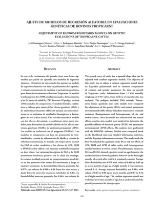
9. AJUSTE DE MODELOS DE REGRESIÓN ALEATORIA EN EVALUACIONES GENÉTICAS DE BOVINOS TROPICARNE
efectos directos de ambiente permanente y maternos permanent environmental effects, and quadratic
(genéticos y de ambiente permanente) de orden cú- order for permanent environmental maternal effects.
bico, con varianzas residuales heterogéneas de doce Nobre et al. (2003a) and Nobre et al. (2003b)
clases y 48 parámetros. used quadratic order MRA in genetic (direct and
En estudios similares Villalba et al. (2000) usaron maternal) and environmental (direct and maternal)
polinomios de Legendre de orden cuadrático para effects for implementation of MRA in estimating
describir el crecimiento predestete de bovinos Sui- variance components, genetic parameters, and
zo Pardo y Pirenaica. Albuquerque y Meyer (2001) prediction of genetic values in Nelore cattle growth.
analizaron el crecimiento entre el nacimiento y los In the growth analysis (2 to 8 years of age) in beef
630 d de edad de bovinos Nelore y seleccionaron cattle breeds, Arango et al. (2004) adjusted a linear
otros modelos con los diferentes criterios. Con LRT order MRA for direct genetic effects and fourth order
y AIC seleccionaron un modelo de quinto orden for animal permanent environmental effects, without
para los efectos directos (genéticos y de ambiente considering maternal effects in the analysis.
permanente) y genéticos maternos, más los efectos
maternos de ambiente permanente de orden cúbico; Estimation of (co)variance components
mientras que con BIC seleccionaron un modelo de and genetic parameters
orden cúbico para los efectos genéticos directos y
maternos, de quinto orden para los efectos directos Based on the selected model, (co)variance
de ambiente permanente y de orden cuadrático para components were estimated for all the random
efectos maternos de ambiente permanente. Nobre et effects, heritabilities of direct genetic effects (h2) and
al. (2003a) y Nobre et al. (2003b) usaron MRA de maternal effects (m2), plus the genetic correlations
orden cuadrático en los efectos genéticos (directos y of direct (rd) and maternal (rm) effects, and the
maternos) y ambientales (directos y maternos) para behavior of the variances and genetic parameters over
implementar MRA en la estimación de componen- time were graphed (Figure 1). Phenotypic variance
tes de varianza, parámetros genéticos y predicción showed a positive trend (Figure 1A), while residual
de valores genéticos en el crecimiento de bovinos variance (Figure 1B) showed quadratic behavior
Nelore. En el análisis de crecimiento (2 a 8 años in the first eight months of growth, with a peak
de edad) en vacas de razas de bovinos para carne, around five months, and then no variation until the
Arango et al. (2004) ajustaron un MRA de orden end of the period. Regarding growth traits, residual
lineal para los efectos genéticos directos y de cuar- variances increased with age (Meyer, 2001; Fischer
to orden para los efectos de ambiente permanente et al., 2004); therefore, modeling the growth curve
del animal, sin considerar los efectos maternos en el can improve partition of the phenotypic variance
análisis. in accordance with the random effects included in
the models (Meyer, 2000; El Faro and Albuquerque,
Estimación de componentes de (co)varianza 2003). If heterogeneity of the residual variances is
y parámetros genéticos not considered, genetic progress may be affected by
an incorrect hierarchy of the bulls and, consequently,
Con base en el modelo seleccionado se estimaron precision in the prediction of genetic values may
componentes de (co)varianza para todos los efectos decrease. Problems caused by variance heterogeneity
aleatorios, las heredabilidades de efectos genéticos can be more serious when referring to residual
directos (h2) y maternos (m2), más las correlaciones variance (Hill, 1984; Garrick and Van Vleck, 1987).
genéticas de efectos directos (rd) y maternos (rm), y se Variances in genetic direct and maternal effects
graficó el comportamiento de las varianzas y de los varied over time (Figure 1C). Variance of direct
parámetros genéticos a través del tiempo (Figura 1). genetic effects showed a positive linear trend.
La varianza fenotípica presentó una tendencia positi- Behavior of the variance of maternal genetic effects
va (Figura 1A), la varianza residual (Figura 1B) pre- was similar to that of a cubic function: between birth
sentó un comportamiento cuadrático en los primeros and six months of age, it had a positive slope, from
ocho meses del crecimiento, con un pico máximo six to 10 months a stationary phase, and as of 11
alrededor de los cinco meses y luego se mantuvo sin months of age the trend was again positive (Figure
DOMÍNGUEZ-VIVEROS et al. 333

10. AGROCIENCIA, 1 de abril - 15 de mayo, 2011
2 2
hd hm
Figura 1. Comportamiento de las varianzas (kg2): (A) fenotípicas; (B) residuales; (C) genéticas aditivas directas ( ) y maternas ( ) y
(D) heredabilidades directas (hd ) y maternas (hm ) durante el crecimiento.
2 2
2
Figure 1. Behavior of variances (kg ): (A) phenotypic; (B) residual; (C) genetic, additive direct ( ) and maternal ( ), (D) direct
(hd2 ) and maternal (hm ) heritabilities during growth.
2
variaciones hasta el final del periodo. Con respecto 1C). Similar behavior in the phenotypic variances
a las características de crecimiento, las varianzas re- and different behavior in genetic and environmental
siduales se incrementan conforme aumentó la edad variances were reported by Albuquerque and Meyer
(Meyer, 2001; Fischer et al., 2004); por consiguiente, (2001) in Nelore cattle and by Arango et al. (2004)
la modelación de la curva de crecimiento puede me- for beef cattle growth.
jorar la partición de la varianza fenotípica de acuerdo Heritability (h2) averaged 0.079 and fluctuated
con los efectos aleatorios incluidos en los modelos between 0.006 and 0.116. Birth weight (PN) had
(Meyer, 2000; El Faro y Albuquerque, 2003). Si no the lowest h2. For weights measured between one
se considera la heterogeneidad de las varianzas resi- and seven months of age, h2 fluctuated between 0.02
duales puede afectarse el progreso genético debido a and 0.06; as of eight months of age, h2 were around
una jerarquización incorrecta de sementales y como 0.11 and remained constant until 24 months of age
consecuencia, puede disminuirse la precisión de la (Figure 1D). The change in h2 in the interval PN
predicción de valores genéticos. Los problemas por to weight at seven months of age is attributable to
heterogeneidad de varianza pueden ser más graves the overestimation of the residual variance of this
cuando se refiere a la varianza residual (Hill, 1984; period (Figure 1B) due to the inclusion of limited
Garrick y Van Vleck, 1987). information Table 1). In our study, the h2 are lower
Las varianzas de efectos genéticos, directos y ma- than those published by Domínguez-Viveros et al.
ternos variaron con el tiempo (Figura 1C). La varian- (2003) and Ramírez-Valverde et al. (2007) using
za de efectos genéticos directos presentó una tenden- the same database for weights at birth, weaning,
cia lineal positiva. El comportamiento de la varianza one year and 18 months of age, with univariate and
334 VOLUMEN 45, NÚMERO 3

11. AJUSTE DE MODELOS DE REGRESIÓN ALEATORIA EN EVALUACIONES GENÉTICAS DE BOVINOS TROPICARNE
de efectos genéticos maternos fue similar al de una multivariate models. The h2 estimated by Ríos (2008)
función cúbica, entre el nacimiento y los seis meses and analyzed by Zerlotti et al. (1995) for beef cattle
el peso (PN) presentó pendiente positiva, de los seis a growth up to preweaning and de Lira et al. (2008) for
los diez meses presentó una fase estacionaria, y desde preweaning and postweaning growth characteristics
los 11 meses de nuevo una fase positiva (Figura 1C). of Zebu breeds, in most cases are higher than those
Comportamientos similares en las varianzas fenotípi- found in our study.
cas y diferentes en las varianzas genéticas y ambien- Maternal effects (m2) varied from 0.017 to 0.159,
tales fueron reportados por Albuquerque y Meyer and their average was 0.084. Between birth and
(2001) en bovinos Nelore y Arango et al. (2004) en seven months of age, they fluctuated between 0.02
el crecimiento de bovinos para carne. and 0.06, and from seven to 18 months exhibited
Las h2 promediaron 0.079 y fluctuaron entre variations from 0.06 to 0.11. As of 18 months of age,
0.006 y 0.116. La h2 menor correspondió a PN. Las the trend was positive and the highest estimation
h2 para los pesos entre uno y siete meses de edad fluc- (0.159) appeared at the end of the evaluated growth
tuaron de 0.02 a 0.06; desde los ocho meses las h2 period (Figure 1D). Estimations of low magnitude
fueron alrededor de 0.11 y constantes hasta los 24 m2, or close to zero, such as those obtained in our
meses de edad (Figura 1D). El cambio de h2 en el study, were reported by Domínguez-Viveros et
intervalo PN hasta el peso en los siete meses de edad al. (2003) and Ramírez-Valverde et al. (2007) in
es atribuible a la sobre estimación de la varianza re- Tropicarne cattle. In general, m2 estimations of our
sidual de ese periodo (Figura 1B) por la información study are lower than average and within the intervals
limitada incluida (Cuadro 1). Las h2 del presente for information analyzed by Zerlotti et al. (1995),
estudio son menores a las publicadas por Domín- de Lira et al. (2008), and Ríos (2008) for genetic
guez-Viveros et al. (2003) y Ramírez-Valverde et al. parameters of growth characteristics of beef cattle.
(2007) con la misma base de datos para pesos en el Nobre et al. (2003a) published different results:
nacimiento, destete, un año y 18 meses de edad, con average h2 of 0.23 and 0.18, with minimums of 0.10
modelos univariados y multivariados. Las estimacio- and 0.12 and maximums of 0.34 and 0.27, m2 of
nes de h2 para el crecimiento de bovinos para carne 0.07 and 0.09 with values of 0.02 and 0.07 to 0.12
hasta el predestete por Ríos (2008) y las analizadas and 0.21, in growth evaluations of Nelore cattle with
por Zerlotti et al. (1995) y de Lira et al. (2008) para two databases.
características de crecimiento predestete y posdestete Direct (rd) and maternal (rm) genetic correlations
en razas cebuinas, en la mayoría de los casos son su- in most of the estimations were positive and above
periores a las del presente estudio. 0.75. However, negative estimations were observed in
Las m2 variaron entre 0.017 y 0.159 y su prome- rd , between PN and weights at one month up to 20
dio fue 0.084. Entre el nacimiento y los siete meses de months of age, with values of 0.002 and 0.128.
edad el peso presentó fluctuaciones de 0.02 a 0.06 y The rd between PN and weights at 21 to 24 months
de los siete a los 18 meses mostró variaciones de 0.06 of age were positive with values between 0.011 and
a 0.11. Desde los 18 meses la tendencia fue positiva y 0.052. The rest of the rd were positive, with values
la estimación máxima (0.159) correspondió con el fi- around 0.99. The rm were positive with values of 0.39
nal del periodo de crecimiento evaluado (Figura 1D). a 0.99. Estimates of rm were the lowest for PN, with
Estimaciones de m2 de magnitud baja y cercanas a values from 0.39 to 0.87. Weights in the preweaning
cero, como las obtenidas en el presente estudio, fue- phase, relative to weights at 20 to 24 months of age,
ron reportadas por Domínguez-Viveros et al. (2003) had rm of around 0.80, and the rm between the most
y Ramírez-Valverde et al. (2007) en bovinos Tropi- distant observations tended to decrease. Regarding
carne. En general, las estimaciones de m2 del presen- the rd, Zerlotti et al. (1995) reported estimations
te estudio son menores al promedio y dentro de los above 0.20 between PN and weights at weaning, one
intervalos de información analizada por Zerlotti et al. year and 18 months of age. Likewise, these authors
(1995), de Lira et al. (2008) y Ríos (2008) de pará- reported rd above 0.45 between weight at weaning
metros genéticos para características de crecimiento and weight at one year and at 18 months of age and
de bovinos para carne. Nobre et al. (2003a) publi- above 0.55 between weight at one year and weight at
caron resultados diferentes: h2 promedio de 0.23 y 18 months of age.
DOMÍNGUEZ-VIVEROS et al. 335

12. AGROCIENCIA, 1 de abril - 15 de mayo, 2011
0.18, con mínimos de 0.10 y 0.12, y máximos de Estimation of variance components and genetic
0.34 y 0.27, m2 de 0.07 y 0.09 con valores de 0.02 y parameters in our study, with values close to
0.07 a 0.12 y 0.21, en evaluaciones del crecimiento zero and lower than those found in the literature
de bovinos Nelore con dos bases de datos. (Zerlotti et al., 195; Ríos, 2008), can be attributed
Las correlaciones genéticas directas (rd) y mater- to three causes. First, the MRA presented erroneous
nas (rm) en la mayoría de las estimaciones fueron estimations at the ends of the growth curves and in
positivas y superiores a 0.75. Sin embargo, se obser- zones with few observations (Nobre et al., 2003b;
varon estimaciones negativas en rd , entre el PN y los Meyer, 2005). Second, the process of estimation is
pesos de un mes hasta los 20 meses de edad, con va- complicated by addition of maternal genetic effects
lores de 0.002 y 0.128. Las rd entre el PN y los and increases when the genetic correlation between
pesos de 21 a 24 meses de edad fueron positivas con direct and maternal effects is considered (Bohmanova
valores entre 0.011 y 0.052. Las demás rd fueron po- et al., 2005). Third, the MRA require robust and
sitivas, con valores alrededor de 0.99. Las rm fueron ample databases, with an adequate distribution
positivas con valores de 0.39 a 0.99. El PN mostró of the observations through all the points to avoid
las estimaciones de rm menores, con valores de 0.39 biased, imprecise estimations (Bohmanova et al.,
a 0.87. Los pesos en la fase predestete, con respecto 2005; Meyer, 2005; Misztal, 2006). Based on the
a los pesos de los 20 a 24 meses de edad, tuvieron above, the peculiarities of the observed results can be
rm alrededor de 0.80 y las rm entre las observaciones attributed to the structure of the database analyzed,
más distantes tendieron a disminuir. Con respecto a with emphasis in the period between two and seven
las rd, Zerlotti et al. (1995) reportaron estimaciones months of age. Furthermore, we suggest analyzing
superiores a 0.20 entre el PN y los pesos al destete, other alternatives (Splines, B-Splines or multivariate
al año y a los 18 meses de edad. Del mismo modo, analyses) for modeling growth curves.
estos autores reportaron rd superiores a 0.45 de peso
al destete con peso al año y a los 18 meses de edad Conclusions
y superiores a 0.55 de peso al año con el de los 18
meses de edad. Growth of Tropicarne cattle, from birth to 24
La estimación de componentes de varianzas y months of age, is best fitted by a random regression
parámetros genéticos en el presente estudio, con model that includes cubic order fixed effects, quadratic
valores cercanos a cero y menores a los de la litera- order direct genetic effects, cubic order permanent
tura (Zerlotti et al. 1995; Ríos, 2008), pueden atri- environmental and maternal (genetic and permanent
buirse a tres causas. Primero, los MRA presentaron environmental) effects, with heterogeneous residual
estimaciones erróneas en los extremos de las curvas variances of twelve classes and 48 parameters. The
de crecimiento, y zonas con observaciones escasas random regression model with the best fit as of nine
(Nobre et al., 2003b; Meyer, 2005). Segundo, la months of age underestimates genetic parameters for
complicación del proceso de estimación por adición younger ages.
de los efectos genéticos maternos, y aumenta cuan-
do se considera la correlación genética entre efectos —End of the English version—
directos y maternos (Bohmanova et al., 2005). Ter-
cero, los MRA requieren bases de datos robustas y pppvPPP
amplias, con distribución adecuada de las observa-
ciones a través de todos los puntos para evitar esti- Conclusiones
maciones sesgadas e imprecisas (Bohmanova et al.,
2005; Meyer, 2005; Misztal, 2006). Con base en lo El crecimiento de bovinos Tropicarne, del naci-
anterior, se puede atribuir a la estructura de la base miento a los 24 meses de edad, se ajusta mejor al
de datos analizada las peculiaridades de los resul- modelo de regresión aleatoria que incluye los efectos
tados observados, con énfasis en el periodo de dos fijos de orden cúbico, los genéticos directos de orden
a siete meses de edad. Además, se sugiere analizar cuadrático, los directos de ambiente permanente y
otras alternativas (Splines, B-Splines o análisis mul- maternos (genéticos y de ambiente permanente) de
tivariados) para modelar la curva de crecimiento. orden cúbico, con varianzas residuales heterogéneas
336 VOLUMEN 45, NÚMERO 3

13. AJUSTE DE MODELOS DE REGRESIÓN ALEATORIA EN EVALUACIONES GENÉTICAS DE BOVINOS TROPICARNE
de doce clases y 48 parámetros. El modelo de regre- Lawrence, T. L. J., and V. R. Fowler. 2002. Growth of Farm
sión aleatoria con mejor ajuste a partir de los nueve Animals. CABI Publishing. 340 p.
Meyer, K. 1998a. Estimating covariance functions for
meses de edad subestima los parámetros genéticos longitudinal data using a random regression model. Genet.
para edades menores. Sel. Evol. 30: 221-240.
Meyer, K. 1998b. DXMRR – A program to estimate covariance
Agradecimientos functions for longitudinal data by REML. Proceeding In:
6th World Congr. Genet. Appl. Livest. Prod. Armidale,
Australia. pp: 465-466.
Se agradece a la Asociación Mexicana de Criadores de Gana-
Meyer, K. 2000. Random regression to model phenotypic
do Tropicarne por facilitar la base de datos genealógica y produc- variation in monthly weights of Australian beef cows. Liv.
tiva para el presente estudio, y al Consejo Nacional de Ciencia y Prod. Sci. 65: 13-38.
Tecnología por la beca proporcionada al primer autor para estu- Meyer, K. 2001. Estimates of direct and maternal covariance
dios de posgrado. function for growth of Australian beef calves from birth to
weaning. Genet. Sel. Evol. 33: 487-514.
Meyer, K. 2005. Random regression analyses using B-splines to
Literatura Citada model growth of Australian Angus cattle. Genet. Sel. Evol.
37: 473-500.
Arango, J. A., L. V. Cundiff, and L. D. Van Vleck. 2004. Misztal, I. 2006. Properties of random regression models using
Covariance functions and random regression models for cow linear splines. J. Anim. Breed. Genet. 123: 74-80.
weight in beef cattle. J. Anim. Sci. 82: 54-67. Nobre, P. R. C., I. Misztal, S. Tsuruta, J. K. Bertrand, L. O.
Albuquerque, L. G., and K. Meyer. 2001. Estimates of covariance C. Silva, and P. S. Lopes. 2003a. Analyses of growth curves
functions for growth from birth to 630 days of age in Nelore of Nellore cattle by multiple-trait and random regression
cattle. J. Anim. Sci. 79: 2776-2789. models. J. Anim. Sci. 81: 918-926.
Bohmanova, J., I. Misztal, and J. K. Bertrand. 2005. Studies Nobre, P. R. C., I. Misztal, S. Tsuruta, J. K. Bertrand, L. O. C.
on multiple trait and random regression models for genetic Silva, and P. S. Lopes. 2003b. Genetic evalution of growth
evaluation of beef cattle for growth. J. Anim. Sci. 83: 62-67. in Nellore cattle by multiple-trait and random regression
Burnham, K. P., and D. R. Anderson. 1998. Model Selection models. J. Anim. Sci. 81: 927-932.
and Inference. Springer. London, UK. 496 p. Ramírez-Valverde, R., O. C. Hernández-Alvarez, R. Núñez-
de Lira, T., E. Maria Rosa, e A. del Valle Garnero. 2008. Domínguez, A. Ruíz-Flores, y J. G. García-Muñiz. 2007.
Parâmetros genéticos de características productivas e Análisis univariado vs. multivariado en la evaluación genética
reproductivas em zebuínos de corte (Revisão). Ciência de variables de crecimiento en dos razas bovinas. Agrociencia
Anim. Bras. 9: 1-22. 41: 271-282.
Domínguez-Viveros, J., F. A. Rodríguez-Almeida, J. A. Ortega- Ríos U., Á. 2008. Estimadores de parámetros genéticos para
Gutiérrez, y A. Flores-Mariñelarena. 2009. Selección de características de crecimiento predestete de bovinos.
modelos, parámetros genéticos y tendencias genéticas, en Revisión. Téc. Pecu. Méx. 46: 37-67.
las evaluaciones genéticas nacionales de bovinos Brangus y Rosales A., J., M. A. Elzo, M. Montaño B., V. E. Vega M., y A.
Salers. Agrociencia 43: 107-117. Reyes V. 2004. Parámetros genéticos para peso al nacimiento
Domínguez-Viveros, J., R. Núñez-Domínguez, R. Ramírez- y destete en ganado Simmental-Brahman en el subtrópico
Valverde, y A. Ruíz-Flores. 2003. Evaluación genética de mexicano. Téc. Pecu. Méx. 42: 333-346.
variables de crecimiento en bovinos Tropicarne: I. Selección Ruíz-Flores, A., R. Núñez-Domínguez, R. Ramírez-Valverde,
de modelos. Agrociencia 37: 323-335. J. Domínguez-Viveros, M. Mendoza-Domínguez,
El Faro, y L. G. Albuquerque. 2003. Utilização de modelos de y E. Martínez-Cuevas. 2006. Niveles y efectos de la
regressão aleatória para produção de leite no dia do controle, consanguinidad en variables de crecimiento y reproductivas
com diferentes estruturas de variâncias residuais. Rev. Bras. en bovinos Tropicarne y Suizo Europeo. Agrociencia 40:
Zootec. 32: 1104-1113. 289-301.
Fischer, T. M., J. H. J. Van der Werf, R. G. Banks, and A. J. Ball. Sakaguti, E. S. 2003. Avaliação do crescimento de bovinos
2004. Description of lamb growth using random regression jovens da raça Tabapuã, por meio de análises de funções de
on field data. Liv. Prod. Sci. 89: 175-185. covariâncias. Rev. Soc. Bras. Zoot. 32: 864-874.
Garrick D. J., and L. D. Van Vleck. 1987. Aspect of selection Schaeffer, L. R. 2004. Application of random regression models
for performance in several environments with heterogeneous in animal breeding. Liv. Prod. Sci. 86: 35-45.
variances. J. Anim. Sci. 65: 409-421. Villalba, D., I. Casasus, A. Sanz, J. Estany, and R. Revilla. 2000.
Henderson, C. R. 1984. Applications of Linear Models in Preweaning growth curves in Brown Swiss and Pirenaica
Animal Breeding. University of Guelph. Guelph, Canada. calves with emphasis o individual variability. J. Anim. Sci.
423 p. 78: 1132-1140.
Hill, W. G. 1984. On selection among groups with heterogeneous Zerlotti M., M. E., R. Barbosa L., y A. de los Reyes B. 1995.
variance. Animal Production 39: 473-477. Parámetros genéticos para características de crecimiento en
Kirkpatrick, M., D. Lofsvold, and M. Bulmer. 1990. Analysis cebuínos de carne. Arch. Latinoam. Prod. Anim. 3: 45-89.
of the inheritance, selection and evolution of growth Zucchini, W. 2000. An introduction to model selection. J.
trajectories. Genetics 124: 979-993. Mathem. Psych. 44: 41-61.
DOMÍNGUEZ-VIVEROS et al. 337