SlideShare una empresa de Scribd logo
1 de 577
Descargar para leer sin conexión
5 63 1.60 59.80 2" Flexible (UF) 7.5 48 1.80 44.40 1 1/2" Simple Presion (SP)
5 75 1.90 71.20 2 1/2" Flexible (UF) 7.5 63 2.30 58.40 2" Flexible (UF)
5 90 2.20 85.60 3" Flexible (UF) 7.5 75 2.80 69.40 2 1/2" Flexible (UF)
5 110 2.70 104.60 4" Flexible (UF) 7.5 90 3.30 83.40 3" Flexible (UF)
5 140 3.50 133.00 5 1/2" Flexible (UF) 7.5 110 4.00 102.00 4" Flexible (UF)
5 160 4.00 152.00 6" Flexible (UF) 7.5 140 5.10 129.80 5 1/2" Flexible (UF)
5 200 4.90 190.20 8" Flexible (UF) 7.5 160 5.80 148.40 6" Flexible (UF)
5 250 6.20 237.60 10" Flexible (UF) 7.5 200 7.30 185.40 8" Flexible (UF)
5 315 7.70 299.60 12" Flexible (UF) 7.5 250 9.10 231.80 10" Flexible (UF)
7.5 315 11.40 292.20 12" Flexible (UF)
10 21 1.80 17.40 1/2" Simple Presion (SP) 15 63 4.40 54.20 2" Flexible (UF)
10 26.5 1.80 22.90 3/4" Simple Presion (SP) 15 75 5.30 64.40 2 1/2" Flexible (UF)
10 33 1.80 29.40 1" Simple Presion (SP) 15 90 6.30 77.40 3" Flexible (UF)
10 42 2.00 38.00 1 1/4" Simple Presion (SP) 15 110 7.70 94.60 4" Flexible (UF)
10 48 2.30 43.40 1 1/2" Simple Presion (SP) 15 140 9.80 120.40 5 1/2" Flexible (UF)
10 63 3.00 57.00 2" Flexible (UF) 15 160 11.20 137.60 6" Flexible (UF)
10 75 3.60 67.80 2 1/2" Flexible (UF) 15 200 14.00 172.00 8" Flexible (UF)
10 90 4.30 81.40 3" Flexible (UF) 15 250 17.50 215.00 10" Flexible (UF)
10 110 5.30 99.40 4" Flexible (UF) 15 315 22.00 271.00 12" Flexible (UF)
10 140 6.70 126.60 5 1/2" Flexible (UF)
10 160 7.70 144.60 6" Flexible (UF)
10 200 9.60 180.80 8" Flexible (UF)
10 250 11.90 226.20 10" Flexible (UF) 160-C2.5 156.00 6" Flexible (UF)
10 315 15.00 285.00 12" Flexible (UF) 200-C2.5 195.00 8" Flexible (UF)
250-C2.5 243.80 10" Flexible (UF)
SP 5 m largo 315-C2.5 307.20 12" Flexible (UF)
UF 6 m largo 355-C2.5 346.20 14" Flexible (UF)
FERNANDO UGAZ ODAR
30/05/2010
2.5
GROSOR
MINIMO DE
PARED (mm)
GROSOR
MINIMO DE
PARED (mm)
ACOPLE CLASE
CLASE
DIAMETRO
NOMINAL (mm)
DIAMETRO
INTERIOR
(mm)
DIAMETRO
NOMINAL
(pulg)
ACOPLE
DIAMETRO
NOMINAL
(pulg)
DIAMETRO
NOMINAL
(mm)
DIAMETRO
INTERIOR
(mm)
ACOPLE
CLASE
DIAMETRO
NOMINAL
(mm)
DIAMETRO
INTERIOR
(mm)
DIAMETRO
NOMINAL
(pulg)
GROSOR
MINIMO DE
PARED (mm)
DIAMETRO
NOMINAL
(pulg)
ACOPLE
DIAMETROS NOMINALES DE TUBERIAS PVC - PRODUCTO PERUANO
ACOPLE CLASE
CLASE
DIAMETRO
NOMINAL (mm)
DIAMETRO
INTERIOR
(mm)
DIAMETRO
NOMINAL
(pulg)
GROSOR
MINIMO DE
PARED (mm)
DIAMETRO
NOMINAL
(mm)
DIAMETRO
INTERIOR
(mm)
//Programa que toma lecturas de los sensores de humedad de suelo cada 5 minutos.
//Se emplean los puertos analogicos y son sensados 2 dispositivos a la vez por sector. Los cuales
miden la humedad que se encuentra en el suelo de los cultivos.
//Lo cual hace activar la válula solenoide del sector para que permitan el ingreso del flujo de agua
a través de estos.
//Caso contrario, cuando se indique el valor de '0' lógico, se envía una señal de control a las
válvula para que se cierre e impida el flujo de agua.
//Posteriormente se procede con regar el siguiente sector y así hasta cubrir todos los sectores de
riego.
int i;
int j;
int pin=1;
int salida;
int aux;
int aux2;
int time;
int minuto;
int analogPin;
int sector;
int swc1;
int swc2;
int valve;
int swcauxmin;
int swcauxmax;
int swcaux;
int ValRef;
int ivwc;
float vwc;
String comand="";
float current;
float vwc1;
float vwc2;
int vwc11;
int vwc12;
int vwc21;
int vwc22;
void setup ()
{ Serial.begin(9600);
for(int pin=2; pin < 10 ; pin++)
{
pinMode(pin, OUTPUT);
}
i=1;
aux=0;
aux2=0;
sector=0;
}
void loop ()
{
//INICIA CICLO DE RIEGO
//PARA COMENZAR SE CIERRAN TODAS LAS VALVULAS
// '0' lógico para desactivar la alimentación del actuador
CalibrarSensor();
for( pin=2; pin < 10 ; pin++)
{
digitalWrite(pin,LOW);
delay(500);
delay(500);
}
//COMIENZA LA IRRIGACIÓN ACTIVANDO LA VALVULA DEL SECTOR 1
pin=2;
aux=0;
analogPin=0;
while(aux < 8)
{
sector++;
digitalWrite(pin,HIGH);
delay(500);
delay(500);
LeerSensor:
PeriodoSensado();
swc1=analogRead(analogPin);
analogPin++;
delay(500);
delay(500);
swc2=analogRead(analogPin);
analogPin++;
delay(500);
delay(500);
vwc1 = CalculaVWC (swc1);
delay(500);
vwc11 = CalculaiVWC (swc1);
delay(500);
vwc2 = CalculaVWC (swc2);
delay(500);
vwc21 = CalculaiVWC (swc2);
delay(500);
vwc1= (vwc1 - vwc11)*100;
delay(500);
vwc2= (vwc2 - vwc21)*100;
delay(500);
vwc12=vwc1;
vwc22=vwc2;
// Realiza la estrategia de control on/off
// compara el nivel de humedad actual con el nivel requerido por las plantas
// Envia el comando generado hacia la interfaz para visualizar los niveles de humedad
if( swc1 <= ValRef || swc2 <= ValRef)
{
valve=1;
EnviarComando();
analogPin=analogPin - 2;
delay(500);
delay(500);
goto LeerSensor;
}
else
{digitalWrite(pin,LOW);
valve=0;
EnviarComando();
delay(500);
delay(500);
}
aux++;
pin++;
}
//Serial.println("*********************************");
//Serial.println("Ya se termino el ciclo de riego ");
//Serial.println("*********************************");
lazo:
goto lazo;
}
// El programa calibrarSensor toma varias muestras del suelo antes de comenzar con el ciclo de
riego para que la toma de datos sea lo mas preciso posible.
// Su rutina consiste en tomar muestras cada 3 segundos durante 5 minutos.
// Se toma muestras cuando el suelo se encuentre totalmente seco y totalmente húmedo, de tal
forma que se pueda establecer el rango de operación del sensor.
// Ademas se toma la muestra cuando se haya aplicado el nivel requerido de agua para el cultivo.
// Estos 3 datos son necesarios para comenzar con el ciclo de riego.
void CalibrarSensor()
{ analogPin=0;
swcaux=0;
swcauxmin=0;
swcauxmax=0;
ValRef=0;
j=0;
// Se calcula el nivel minimo de humedad de suelo
for(aux=1;aux<=100;aux++)
{ j++;
swcaux=analogRead(analogPin);
swcauxmin=(swcauxmin+swcaux)/j;
delay(1500);
delay(1500);
}
//Se calcula el nivel maximo de humedad de suelo
j=0;
for(aux=1;aux<=100;aux++)
{ j++;
swcaux=analogRead(analogPin);
swcauxmax=(swcauxmax+swcaux)/j;
delay(1500);
delay(1500);
}
//Se calcula el nivel de referencia de humedad de suelo
j=0;
for(aux=1;aux<=100;aux++)
{ j++;
swcaux=analogRead(analogPin);
ValRef=(ValRef+swcaux)/j;
delay(1500);
delay(1500);
}
}
// Rutina que genera un retardo para la toma de datos.
// 5 minutos
//
void PeriodoSensado()
{ time=0;
//36 3 min
for(time=1;time <= 36;time++)
{ delay(500);
delay(500);
delay(500);
delay(500);
delay(500);
delay(500);
delay(500);
delay(500);
delay(500);
delay(500);
}
}
//Envia el comando generado por el arduino para el monitoreo del sistema de riego en la interfaz
grafica de labview.
//Requiere los siguientes parametros: # de sector de riego, Nivel de humedad de suelo 1 , Nivel de
humedad de suelo 2 , estado de valvula (abierta o cerrada)
void EnviarComando()
{ comand = 0;
comand += "S";
comand += sector;
comand += ",";
comand += vwc11;
comand += ".";
comand += vwc12;
comand += ",";
comand += vwc21;
comand += ".";
comand += vwc22;
comand += ",";
comand += valve;
delay (500);
delay (500);
Serial.println(comand);
}
//Esta funcion recibe como entrada el valor digital del sensor y convierte la señal en las unidades
//que se emplea en el cultivo de riego.
// Contenido volumetrico de agua
// Ambos calculan el mismo nivel, lo que diferencia es el tipo de variable
float CalculaVWC(int digital_value)
{
current = digital_value * 0.01953125;
vwc = 4.25 * current - 34.2;
return vwc;
}
int CalculaiVWC(int digital_ivalue)
{
current = digital_ivalue * 0.01953125;
ivwc = 4.25 * current - 34.2;
return ivwc;
}
2N2219A
2N2222A
HIGH SPEED SWITCHES
PRELIMINARY DATA
DESCRIPTION
The 2N2219A and 2N2222A are silicon Planar
Epitaxial NPN transistors in Jedec TO-39 (for
2N2219A) and in Jedec TO-18 (for 2N2222A)
metal case. They are designed for high speed
switching application at collector current up to
500mA, and feature useful current gain over a
wide range of collector current, low leakage
currents and low saturation voltage.
®
INTERNAL SCHEMATIC DIAGRAM
February 2003
ABSOLUTE MAXIMUM RATINGS
Symbol Parameter Value Unit
VCBO Collector-Base Voltage (IE = 0) 75 V
VCEO Collector-Emitter Voltage (IB = 0) 40 V
VEBO Emitter-Base Voltage (IC = 0) 6 V
IC Collector Current 0.6 A
ICM Collector Peak Current (tp < 5 ms) 0.8 A
Ptot Total Dissipation at Tamb ≤ 25 o
C
for 2N2219A
for 2N2222A
at TC ≤ 25
o
C
for 2N2219A
for 2N2222A
0.8
0.5
3
1.8
W
W
W
W
Tstg Storage Temperature -65 to 175 o
C
Tj Max. Operating Junction Temperature 175 o
C
TO-18 TO-39
1/7
THERMAL DATA
TO-39 TO-18
Rthj-case
Rthj-amb
Thermal Resistance Junction-Case Max
Thermal Resistance Junction-Ambient Max
50
187.5
83.3
300
o
C/W
o
C/W
ELECTRICAL CHARACTERISTICS (Tcase = 25 o
C unless otherwise specified)
Symbol Parameter Test Conditions Min. Typ. Max. Unit
ICBO Collector Cut-off
Current (IE = 0)
VCB = 60 V
VCB = 60 V Tj = 150 o
C
10
10
nA
µA
ICEX Collector Cut-off
Current (VBE = -3V)
VCE = 60 V 10 nA
IBEX Base Cut-off Current
(VBE = -3V)
VCE = 60 V 20 nA
IEBO Emitter Cut-off Current
(IC = 0)
VEB = 3 V 10 nA
V(BR)CBO Collector-Base
Breakdown Voltage
(IE = 0)
IC = 10 µA 75 V
V(BR)CEO∗ Collector-Emitter
Breakdown Voltage
(IB = 0)
IC = 10 mA 40 V
V(BR)EBO Emitter-Base
Breakdown Voltage
(IC = 0)
IE = 10 µA 6 V
VCE(sat)∗ Collector-Emitter
Saturation Voltage
IC = 150 mA IB = 15 mA
IC = 500 mA IB = 50 mA
0.3
1
V
V
VBE(sat)∗ Base-Emitter
Saturation Voltage
IC = 150 mA IB = 15 mA
IC = 500 mA IB = 50 mA
0.6 1.2
2
V
V
hFE∗ DC Current Gain IC = 0.1 mA VCE = 10 V
IC = 1 mA VCE = 10 V
IC = 10 mA VCE = 10 V
IC = 150 mA VCE = 10 V
IC = 500 mA VCE = 10 V
IC = 150 mA VCE = 1 V
IC = 10 mA VCE = 10 V
Tamb = -55 o
C
35
50
75
100
40
50
35
300
hfe∗ Small Signal Current
Gain
IC = 1 mA VCE = 10 V f = 1KHz
IC = 10 mA VCE = 10 V f = 1KHz
50
75
300
375
fT Transition Frequency IC = 20 mA VCE = 20 V
f = 100 MHz
300 MHz
CEBO Emitter-Base
Capacitance
IC = 0 VEB = 0.5 V f = 100KHz 25 pF
CCBO Collector-Base
Capacitance
IE = 0 VCB = 10 V f = 100 KHz 8 pF
Re(hie) Real Part of Input
Impedance
IC = 20 mA VCE = 20 V
f = 300MHz
60 Ω
* Pulsed: Pulse duration = 300 µs, duty cycle ≤ 1 %
2N2219A / 2N2222A
2/7
ELECTRICAL CHARACTERISTICS (continued)
Symbol Parameter Test Conditions Min. Typ. Max. Unit
NF Noise Figure IC = 0.1 mA VCE = 10 V
f = 1KHz Rg = 1KΩ
4 dB
hie Input Impedance IC = 1 mA VCE = 10 V
IC = 10 mA VCE = 10 V
2
0.25
8
1.25
kΩ
kΩ
hre Reverse Voltage Ratio IC = 1 mA VCE = 10 V
IC = 10 mA VCE = 10 V
8
4
10-4
10
-4
hoe Output Admittance IC = 1 mA VCE = 10 V
IC = 10 mA VCE = 10 V
5
25
35
200
µS
µS
td∗∗ Delay Time VCC = 30 V IC = 150 mA
IB1 = 15 mA VBB = -0.5 V
10 ns
tr∗∗ Rise Time VCC = 30 V IC = 150 mA
IB1 = 15 mA VBB = -0.5 V
25 ns
ts∗∗ Storage Time VCC = 30 V IC = 150 mA
IB1 = -IB2 = 15 mA
225 ns
tf∗∗ Fall Time VCC = 30 V IC = 150 mA
IB1 = -IB2 = 15 mA
60 ns
rbb’ Cb’c Feedback Time
Constant
IC = 20 mA VCE = 20 V
f = 31.8MHz
150 ps
∗ Pulsed: Pulse duration = 300 µs, duty cycle ≤ 1 %
∗∗ See test circuit
2N2219A / 2N2222A
3/7
Test Circuit fot td, tr.
PULSE GENERATOR : TO OSCILLOSCOPE
tr ≤ 20 ns tr ≤ 5.0 ns
PW ≤ 200 ns ZIN < 100 KΩ
ZIN = 50 Ω CIN ≤ 12 pF
Test Circuit fot td, tr.
PULSE GENERATOR : TO OSCILLOSCOPE :
PW ≈ 10 µs tr < 5.0 ns
ZIN = 50 Ω ZIN > 100 KΩ
TC ≤ 5.0 ns CIN ≤ 12 pF
2N2219A / 2N2222A
4/7
DIM.
mm inch
MIN. TYP. MAX. MIN. TYP. MAX.
A 12.7 0.500
B 0.49 0.019
D 5.3 0.208
E 4.9 0.193
F 5.8 0.228
G 2.54 0.100
H 1.2 0.047
I 1.16 0.045
L 45o
45o
L
G
I
D A
F
E
B
H
C
TO-18 MECHANICAL DATA
0016043
2N2219A / 2N2222A
5/7
DIM.
mm inch
MIN. TYP. MAX. MIN. TYP. MAX.
A 12.7 0.500
B 0.49 0.019
D 6.6 0.260
E 8.5 0.334
F 9.4 0.370
G 5.08 0.200
H 1.2 0.047
I 0.9 0.035
L 45o
(typ.)
L
G
I
D A
F
E
B
H
P008B
TO-39 MECHANICAL DATA
2N2219A / 2N2222A
6/7
Information furnished is believed to be accurate and reliable. However, STMicroelectronics assumes no responsibility for the consequences
of use of such information nor for any infringement of patents or other rights of third parties which may result from its use. No license is
granted by implication or otherwise under any patent or patent rights of STMicroelectronics. Specification mentioned in this publication are
subject to change without notice. This publication supersedes and replaces all information previously supplied. STMicroelectronics products
are not authorized for use as critical components in life support devices or systems without express written approval of STMicroelectronics.
The ST logo is a trademark of STMicroelectronics
© 2003 STMicroelectronics – Printed in Italy – All Rights Reserved
STMicroelectronics GROUP OF COMPANIES
Australia - Brazil - Canada - China - Finland - France - Germany - Hong Kong - India - Israel - Italy - Japan - Malaysia - Malta - Morocco -
Singapore - Spain - Sweden - Switzerland - United Kingdom - United States.
http://www.st.com
2N2219A / 2N2222A
7/7
This datasheet has been download from:
www.datasheetcatalog.com
Datasheets for electronics components.
RESULTADOS DE LA LÓGICA DE CONTROL
Lecturas digitales del sensor analógico.
Se aprecia que cada vez que transcurre un periodo de muestreo, el Arduino Mega genera un
comando con la información recibida y lo envía a través de la comunicación serial hacia la Interfaz
Gráfica del Usuario desarrollado en el software Labview 2012 de la empresa National Instruments.
En este comando generado por el controlador, se puede observar que indica el número de sector
en el cual se encuentra el proceso de riego. Posteriormente la lectura de los sensores que se
encuentran distribuidos en tal sector, y por último, el estado lógico en el que se encuentra la
válvula solenoide.
Según la lógica de control del proceso de riego, este cambia de sector de riego si es que se supera
el nivel de referencia de humedad de suelo. En este caso se estableció que el mencionado Set
Point sea de 700, por tal razón se puede apreciar que una vez que supere el nivel indicado, la
lógica de control cambia y realiza la acción de apagar la válvula con un estado lógico de ‘0’, esto se
puede apreciar en el último comando generado en referencia al sector de riego 1. Luego se
procede con la apertura de la válvula del segundo sector de riego, así sucesivamente hasta cubrir
todo el terreno.
PROGRAMA PRINCIPAL
INTERFAZ GRAFICA DE USUARIO
Se presenta algunas imágenes que fueron tomadas mientras se realizaba las pruebas del diseño
electrónico.
Anexo 6
En el presente anexo se explica el diseño de la etapa de alimentación para la operación de
la válvula solenoide. En el figura 1, se observa el circuito de simulación el cual consiste en
una fuente de voltaje de corriente alterna (AC), configurada a 220 VAC y una frecuencia de
60 Hz. La siguiente etapa conformada por 4 diodos 1N4001 se conoce como rectificación
de señal a onda completa, dicha etapa realiza la conversión de una señal AC a una señal
DC. Por último, la resistencia R1 y el condensador C1 completan la conversión de la señal
alterna disminuyendo el voltaje de rizado que se genera en la etapa de rectificación.
Figura 1. Circuito de prueba
En la figura anterior, se observa el circuito realizado en el software SpiceNet mediante el
cual se puede analizar el voltaje de rizado que se genera en la punta de medición Y1.
También se puede visualizar la señal de entrada de voltaje alterna V1 mediante la punta
Y2, con el objetivo de asegurarse que la señal de entrada sea la correcta.
1
2
V1
2
2
1
1
1 3
D1
1N4001
2 3
D2
1N4001
2
D3
1N4001
1
D4
1N4001
1 1
1
1
1 1
3
C1
630u
3 3 3
3
3
3
1 1
1
1
1
1
1
1
2
2
2
2
2
2
2
2
3
Y1

+
-
2
1
Y2
2 2
1
1
1 1
2
2
3
R1
32
3
3
3 3
En la figura 2, se puede observar las gráficas generadas por la simulación del circuito desarrollado. Esto mediante la herramienta Scope del
software SpiceNet.
Figura 2. Gráficas de voltaje de entrada y salida del circuito de prueba.
De la figura 2, se obtiene que la señal rectificada presente un voltaje de rizado de menor a
un 1 voltio, aproximadamente 856 mV, lo cual es adecuado para diseños eléctricos ya que
no supera el 5% del Voltaje pico de la señal. Sin embargo, dicho rango se encuentra fuera
del rango de alimentación de la carga, en el presente trabajo de tesis se trata en una
válvula solenoide; por esta razón, se requiere de una etapa que pueda brindar el
suficiente voltaje como para alimentar la válvula solenoide, el cual consiste en adicionar
un regulador de voltaje para que garantice el nivel de voltaje adecuado.
Figura 3. Diseño del circuito de alimentación de la válvula solenoide.
De esta forma, se realiza el diseño de alimentación de la electro – válvula tal y como se
muestra en la figura 3; considerando su los efectos que se generan en la etapa de
rectificación de una señal alterna, como también el rango de alimentación del actuador
mecánico-eléctrico.
ECH2O EA-10
Soil Moisture Sensor
Integrator’s Guide
Version 3
Decagon Devices, Inc.
All rights reserved
©2008-2011
Decagon Devices, Inc.
2365 NE Hopkins Court
Pullman W
A 99163
www.decagon.com
EA-10 Soil Moisture Sensor Integrator’s Guide
i
Contents
1. Introduction . . . . . . . . . . . . . . 1
Specifications . . . . . . . . . . . . . . . . . . . . . . . . . . . . 1
Contact Information. . . . . . . . . . . . . . . . . . . . . . . 2
Warranty Information . . . . . . . . . . . . . . . . . . . . . 2
2. Installing the EA-10 . . . . . . . 4
Procedure . . . . . . . . . . . . . . . . . . . . . . . . . . . . . . . 4
Orientation. . . . . . . . . . . . . . . . . . . . . . . . . . 5
Turf Installation . . . . . . . . . . . . . . . . . . . . . . 5
Removing the Probe . . . . . . . . . . . . . . . . . . 6
Electrical Connection . . . . . . . . . . . . . . . . . . . . . 7
Hardware Requirements . . . . . . . . . . . . . . . . . . . 8
Troubleshooting . . . . . . . . . . . . . . . . . . . . . . . . . . 8
3. How the EA-10 Works . . . . 10
Calibration . . . . . . . . . . . . . . . . . . . . . . . . . . . . . . 11
Functional Testing . . . . . . . . . . . . . . . . . . . . . . . . 11
4. Further Reading . . . . . . . . 12
Index . . . . . . . . . . . . . . . . . . . . 13
EA-10 Soil Moisture Sensor Integrator’s Guide
1. Introduction
1
1. Introduction
Thank you for using the ECH2O EA-10 Dielectric
Soil Moisture sensor. The EA-10 sensor has a stan-
dard 2-wire, 4-20 mA analog interface for use with
industrial data acquisition and control systems.
Specifications
Model: EA-10 Dielectric Soil Moisture Sensor.
Electrical specs:
Interface: 4-20 mA, 2-wire analog transmitter
Red: (+) supply; Black: (-) supply; Shield: NC
Supply voltage: line powered 7-32 Volt; DC
Overvoltage and reverse polarity protected
Sensor Specification:
Measurement type: Volumetric Water Content (VWC)
Measurement range: typical 0 to 40 percent VWC
Measurement resolution: depends on acquisition hardware
Measurement accuracy: ± 2% with soil specific calibra
tion; accuracy at standard factory calibration varies
depending on soil type
Measurement output: current linearly related to VWC.
Active sensor length: 10 cm
Minimum measurement time: 10 ms
Soils: all types; coarse sand to clay
EA-10 Soil Moisture Sensor Integrator’s Guide
1. Introduction
2
Operating environment:
Temperature: -40 to +50 °C.
Humidity: 0-100%
Physical properties:
Dimensions: 14.5cm x 3.17cm x 0.15 cm
Cable: 2 meter, 26 AWG tinned, bare wire (Custom
length available upon request. Cost depends on length).
Calibration:
Percent Volumetric Water Content = 0.0425 x current
(mA)-0.342
Functional testing:
Sensor output in air: 4.0-5.5 mA
Sensor output in water: 16.0-18.5 mA.
Contact Information
If you need to contact Decagon:
• E-mail us at support@decagon.com
• Send us a fax at (509) 332-5158
• Call us at: (US and Canada only) 1-800-755-2751
or 509-332-2756.
Warranty Information
The EA-10 has a 30-day satisfaction guarantee and a
one-year warranty.
EA-10 Soil Moisture Sensor Integrator’s Guide
1. Introduction
3
Seller’s Liability
Seller warrants new equipment of its own manufacture
against defective workmanship and materials for a
period of one year from date of receipt of equipment
(the results of ordinary wear and tear, neglect, misuse,
accident and excessive deterioration due to corrosion
from any cause are not to be considered a defect); but
Seller’s liability for defective parts shall in no event
exceed the furnishing of replacement parts F.O.B. the
factory where originally manufactured. Material and
equipment covered hereby which is not manufactured
by Seller shall be covered only by the warranty of its
manufacturer. Seller shall not be liable to Buyer for
loss, damage or injuries to persons (including death),
or to property or things of whatsoever kind (including,
but not without limitation, loss of anticipated profits),
occasioned by or arising out of the installation, opera-
tion, use, misuse, nonuse, repair, or replacement of
said material and equipment, or out of the use of any
method or process for which the same may be
employed. The use of this equipment constitutes
Buyer’s acceptance of the terms set forth in this war-
ranty. There are no understandings, representations, or
warranties of any kind, express, implied, statutory or
otherwise (including, but without limitation, the
implied warranties of merchantability and fitness for a
particular purpose), not expressly set forth herein.
EA-10 Soil Moisture Sensor Integrator’s Guide
2. Installing the EA-10
4
2. Installing the EA-10
The EA-10 monitors the water content of the soil in
which it is placed by measuring the dielectric constant
of the soil and water surrounding the probe. While the
probe measures just the soil which is adjacent to it, its
reading is most useful if that measurement represents
the general soil conditions in which the probe is
placed. For that to happen, the monitoring site must
be carefully selected, and the probe must be properly
installed.
Procedure
When installing the EA-10 probe, it is best to maxi-
mize contact between the probe and the soil. There
are two methods to accomplish this.
1. Use Decagon’s Probe Installation Kit to install the
probe. This kit has a custom-shaped blade to make
the insertion in the soil, then another tool to place
the probe into the insertion. For deeper installa-
tions, use an augur to reach the desired depth,
then use the Installation kit with extension rods to
install the probe.
2. Use a thin implement like a trenching shovel, gar-
dening spade, or flat bar to make a pilot hole in the
soil. Then insert the probe into the hole, making
sure the entire length of the probe is covered.
Finally, insert the shovel again into the soil a few
inches away from the probe, and gently force soil
toward the probe to provide good contact
at a 45° angle to the ground, instead of straight down.
EA-10 Soil Moisture Sensor Integrator’s Guide
2. Installing the EA-10
5
between the probe and the soil. For deeper instal-
lation, excavate down to the level you wish to mea-
sure, then install the probe as described.
When selecting a site for installation, it is important to
remember that the soil adjacent to the probe surface
has the strongest influence on the probe reading and
that the probe measures the volumetric water content.
Therefore any air gaps or excessive soil compaction
around the probe can profoundly influence the read-
ings. Also, do not install the probes adjacent to large
metal objects such as metal poles or stakes. This can
attenuate the probe’s electromagnetic field and
adversely affect output readings.
Orientation
The probe can be oriented in any direction. However,
orienting the flat side perpendicular to the surface of
the soil will minimize effects on downward water
movement.
Turf Installation
When installing the EA-10, the installation procedure
is almost the same, except that the probe is ofteplaced
break internal connections and make the probe unus-
EA-10 Soil Moisture Sensor Integrator’s Guide
2. Installing the EA-10
6
Removing the Probe
When removing the probe from the soil, do not
pull it out of the soil by the cable! Doing so may
able.
45°
1.0"
Ground Level
EA-10 Soil Moisture Sensor Integrator’s Guide
2. Installing the EA-10
7
Electrical Connection
The EA-10 is a 2 wire, 4 - 20 mA transmitter. When
connected to a 7 - 32 volt source (line power), the cur-
rent is linearly proportional to the water content of the
soil.
The red wire is connected to the positive terminal and
the black wire is the return for the negative terminal.
The shield (bare wire) can be connected to a shield
terminal, if available, or left open. The probe is electri-
ECH2
O EA-10
Soi
lM oi
sture Sensor •4-20 m A transm i
tter
Patent 6904789 R1-05
DECAGON
DEVICES
www.decagon.com
®
7 to 36 Volt DC Source
Red
Wire
Black
Wire
Current Sense Circuit
4–20 mA Analog Hardware
Shield Wire to Ground
EA-10 Soil Moisture Sensor Integrator’s Guide
2. Installing the EA-10
8
cally floating, and the shield is not electrically con-
nected to the probe circuitry. Extension wire can be
used to connect the EA-10 to the 4-20 mA receiver.
The extension wire should be a 2 conductor shielded,
direct burial cable.
NOTE: It is essential that sensor wire connec-
tions be watertight! Use wire nuts with grease or
silicon gel caps for all splices.
Hardware Requirements
The EA-10 is designed to work with industrial control
and acquisition devices. The EA-10 is loop powered,
drawing its operational power from the current used
to measure volumetric water content. Any device
capable of producing a 7 - 32 mA loop voltage should
be compatible with the EA-10. The EA-10 is also
reverse-polarity protected. If it is installed in the
wrong direction, it will not operate, but will be pro-
tected from electrical overload.
NOTE: The EA-10 is intended for use with indus-
trial control and acquisition devices which can
provide a short pulse, leaving the probes turned
off most of the time. Continuous power may
cause the probe to exceed government FCC limits
on electromagnetic emissions.
EA-10 Soil Moisture Sensor Integrator’s Guide
2. Installing the EA-10
9
Troubleshooting
If you encounter problems with the EA-10, they will
usually be in the form of negative or erroneous VWC
readings. The most common solution to this problem
is to make sure that you have adequate probe-to-soil
contact. When inserted, the EA-10 should be com-
pletely covered up to the black overmolding. Doing
this should remedy any reading errors. If it does not,
please contact Decagon for assistance.
EA-10 Soil Moisture Sensor Integrator’s Guide
3. How the EA-10 Works
10
3. How the EA-10 Works
In essence, the EA-10 monitors the water budget of
the soil in which it is placed. It senses water addition
and water loss. If the soil is too wet, irrigation can be
stopped. If the soil becomes too dry, additional irriga-
tion time can be programmed.
Proper monitoring of the water budget requires that
the moisture sensor be located in the active root zone
of relatively homogeneous vegetation, and in well-
drained soil of above-average moisture holding capac-
ity. Avoid locations where water can run-on or pool,
and locations with poor vegetative cover, or where
vegetation tends to water stress because of poor mois-
ture holding capacity of the soil or shallow root zone.
Vegetation in non-monitored zones will use water at a
rate proportional to water use in the monitored zone.
Water application rates in these zones must therefore
be proportional for the entire system to remain prop-
erly irrigated. If trees use 30% more water than turf,
and turf is being monitored, then the tree zone needs
to be irrigated for 30% more time than the monitored
turf to maintain adequate soil moisture.
Since dielectric probes (such as the EA-10) measure
the moisture in the immediate vicinity of the probe, it
is essential that the probe be installed so that the entire
length of the probe is in intimate contact with the soil
EA-10 Soil Moisture Sensor Integrator’s Guide
3. How the EA-10 Works
11
(no air gaps). The soil must therefore be packed tightly
around the entire probe length during installation. The
probe is installed with the blade perpendicular to the
surface to interfere as little as possible with water
movement through the soil.
Calibration
The probe reading is converted to volumetric water
content using the following equation:
Volumetric Water Content = 0.0425 x Current (mA)- 0.342
Water content is in m3
m-3
, and current is in milli-
amps. For water content in terms of percent of total
volume, use the following equation:
Volume percent = 4.25 x Current - 34.2.
These calibrations are for typical soils with mid range
texture, and are accurate enough for most irrigation
scheduling purposes. For greater accuracy, a soil spe-
cific calibration should be undertaken, as outlined on
the Decagon website.
Functional Testing
ECH2O EA-10 sensors are tested to perform cor-
rectly in the following conditions:
Sensor output in air: 4.0-5.5 mA
Sensor output in distilled water: 16.0-18.5mA
EA-10 Soil Moisture Sensor Integrator’s Guide
4. Further Reading
12
4. Further Reading
ECH2O Probes Soil-Specific Calibration
http://www.decagon.com/ag_research/literature/
app_notes.php
ECH2O Dielectric Probes vs. Time Domain
Reflectometers (TDR)
http://www.decagon.com/ag_research/literature/
app_notes.php
ECH2O Probe insertion guide
http://www.decagon.com/ag_research/literature/
app_notes.php
EA-10 Soil Moisture Sensor Integrator’s Guide
Index
13
Index
C
Calibration 11
Contact information 2
F
Functional testing 11
I
Installation
electrical connection 7
hardware requirements 8
procedure 4
S
Seller’s Liability 2
Specifications 1
T
Troubleshooting 8
W
Warranty 2
Electroválvulas
servoaccionadas de 2/2 vías
Modelo EV220B
DN 6-22
DKACV.PD.200.C3.05
520B1636
Mayo 2003
Especificaciones técnicas
DKACV.PD.200.C3.05 Danfoss A/S 05-2003
2
1
/4
- 1” NPT
• Para aplicaciones industriales severas
• Para agua, aceite, aire comprimido y
fluidos neutros similares
• Rango de caudal de agua: 0,2 - 19 m3/h
• Presión diferencial: Hasta 30 bar
• Viscosidad: Hasta 50 cSt
• Temperatura ambiente: Hasta 80°C
• Protección de la bobina: Hasta IP 67
• Conexiones de la rosca: Desde 1
/4
hasta
1” NPT
• Disponible también con rosca G. Por
favor, póngase en contacto con Danfoss.
• Versiones NC en EPDM con aprobación
WRAS
Dimensiones y peso
Opciones de la bobina
Válvula servoaccionada de 2/2 vías
Modelo EV220B
para líquidos y gases neutros
DN 6 -22 B
Desactivada
cerrada
Características
Datos técnicos
1
) Los tiempos son indicativos y se aplican para agua. Los tiempos exactos dependerán de las
condiciones de presión.
Modelo EV220B 6 B EV220B 10 B EV220B 12 B EV220B 18B EV220B 22B
Instalación Serecomiendaunsistema deelectroválvulasvertical (véaseDKACV.PT.600.A)
Rango de presión 0.1 - 30 bar
Max. presión de prueba EV220B 6 -10 B: 50 bar. EV220B 12-22 B: 16 bar
Tiempo de apertura 1
) 40 ms 50 ms 60 ms 200 ms 200 ms
Tiempo de cierre 1
) 250 ms 300 ms 300 ms 500 ms 500 ms
Temperatura ambeiente 40 - 80°C (dependiendo del mod. de bobina, véanse los datos de la bobina seleccionada)
Temperatura del fluido EPDM: -30 a + 100°C. FKM: De 0 a + 100°C
Viscosidad max. 50 cSt
Materiales Cuerpo de la válvula: Latón, n o
. 2.0402
Armadura: Acero inoxidable n o
. 1.4105/AISI 430FR
Tubo de la armadura: Acero inoxidable n o
. 1.4306/AISI 304L
Tope de la armadura: Acero inoxidable n o
. 1.4105/AISI 430FR
Muelles: Acero inoxidable n o
. 1.4310/AISI 301
Juntas tóricas: EPDM o FKM
Clapet: EPDM o FKM
Diafragma: EPDM o FKM
Modelo: BA
9 W ca
15 W cc
Modelo:BB
10 W ca
18W cc
Modelo: BE (IP67)
10 W ca
18 W cc
Modelo: BG
12 W ac
20 W dc
Danfoss dispone de bobinas
exentas de ruidos para aplicaciones
sensibles a los mismos, y también de
bobinas EEx m II T4 para su utilización
en áreas con riesgo de explosión -
para más información consulte la hoja
dedatosDKACV.PD.600.A
Véase DKACV.PD.600.A
Modelo
L B B 1 [mm] H1 H Peso
Modelodebobina Modelodebobina Modelodebobina sin bobina
[mm] [mm] BA/BD BB/BE BG [mm] [mm] [kg]
EV220B 6B 45.5 43.5 32 46 68 13.0 74.0 0.22
EV220B 10B 51.5 48.0 32 46 68 13.0 77.0 0.29
EV220B 12B 58.0 54.0 32 46 68 13.0 77.0 0.35
EV220B 18B 90.0 62.0 32 46 68 18.0 83.0 0.65
EV220B 22B 90.0 62.0 32 46 68 18.0 98.0 0.65
DKACV.PD.200.C3.05-NPT Danfoss A/S 05-2003 3
Desactivada
cerrada
1
/4
“- 1” NPT
Función Tensión de bobina desconectada (cerrada):
Cuando la tensión de la bobina (8) está
desconectada, el muelle de la armadura (1)
presiona el clapet (3) contra el orificio del
piloto (6). La presión a lo largo del diafragma
(7) se crea mediante el orificio de
compensación (4). El diafragma cierra el
orificio principal (5) tan pronto como la
presión del diafragma es equivalente a la
presión de entrada. La válvula permanecerá
cerrada mientras la tensión de la bobina esté
desconectada.
Tensión de la bobina conectada (abierta):
Cuando se aplica tensión a la bobina, se abre
el orificio piloto (6). Como el orificio piloto es
mayor que el orificio de compensación (4), la
presión a lo largo del diafragma (7) cae y así
se eleva libre del orificio principal (5). Ahora la
válvula está abierta y permanecerá así
mientras se mantenga la presión diferencial
mínima a lo largo de la válvula y mientras se
aplique tensión a la válvula.
1. Muelle de la armadura
2. Armadura
3. Clapet
4. Orificio de compensación
5. Orificio principal
6. Orificio piloto
7. Diafragma
8. Bobina
Pedidos: cuerpo de la válvula
Válvula servoaccionada de 2/2 vías
Modelo EV220B
para líquidos y gases neutros
DN 6 -22 B
1
) Indicado sólo para agua.
2
) Indicado para aceite y aire. También se puede utilizar para agua y soluciones acuosas neutras siempre y cuando la temperatura del agua
no exceda de 60 °C.
= sólo gas
Pedidos: bobinas
Véase en las especificaciones técnicas separadas las bobinas DKACV.PD.600.A
Conexión Material Valor Temp. Codigo de Presióndiferencialpermisible[bar]/Modelodebobina
de junta k v de fluido Selección del modelo bobina Min. Max.
NPT
[m3
/h]
A
B
.
x
á
M
.
n
i
M BB/BE BG
[°C] [°C] Modelo principal Especificación Standard)
9 W 15 W 10 W 18 W 12 W 20 W
ca cc ca cc ca cc
3
/8 EPDM 1
) 0.7 -30 +100 EV220B 6 B N 38E NC000 032U7514 0.1 20 - 20 10 20 20
3
/8 FKM 2
) 0.7 0 +100 EV220B 6 B N 38F NC000 032U7516
0.1 20 - 20 10 20 20
0.1 30 - 30 - 30 30
3
/8 EPDM 1
) 1.5 -30 +100 EV220B 10 B N 38E NC000 032U7517 0.1 20 - 20 10 20 20
3/8 FKM 2
) 1.5 0 +100 EV220B 10 B N 38F NC000 032U7519
0.1 20 - 20 10 20 20
0.1 30 - 30 - 30 30
1/2 EPDM 1
) 1.5 -30 +100 EV220B 10 B N 12E NC000 032U7518 0.1 20 - 20 10 20 20
1
/2 FKM 2
) 1.5 0 +100 EV220B 10 B N 12F NC000 032U7520
0.1 20 - 20 10 20 20
0.1 30 - 30 - 30 30
1
/2 EPDM 1
) 2.5 -30 +100 EV220B 12 B N 12E NC000 032U7521 0.3 10 - 10 - - 10
1
/2 FKM 2
) 2.5 0 +100 EV220B 12 B N 12F NC000 032U7522 0.3 10 - 10 - - 10
3
/4 EPDM 1
) 6.0 -30 +100 EV220B 18B N 34E NC000 032U7523 0.3 10 - 10 - 10 10
3/4 FKM 2) 6.0 0 +100 EV220B 18B N 34F NC000 032U7524 0.3 10 - 10 - 10 10
1 EPDM 1) 6.0 -30 +100 EV220B 22B N 1E NC000 032U7525 0.3 10 - 10 - 10 10
1 FKM2) 6.0 0 +100 EV220B 22B N 1F NC000 032U7526 0.3 10 - 10 - 10 10
DKACV.PD.200.C3.05 Danfoss A/S 05-2003
4
G 3
/8
G 1
/2
Instalación Se recomienda un sistema de electroválvulas vertical, véase DKACV.PT.600.A
Rango de presión 0,1 - 10 bar
Máx. presión de prueba 50 bar
Tiempo de apertura 1
) EV220 6 B: 40 ms EV220 10 B: 50 ms
Tiempo de cierre 1
) EV220 6 B: 250 ms EV220 10 B: 300 ms
Temperatura ambiente máx. 80°C (dependiendo del mod. de bobina, véanse los datos de la bobina seleccionada)
Temperatura del fluido EPDM: -30 +100 °C. FKM: 0 - +100 °C
Viscosidad máx. 50 cSt
Materiales Cuerpo de la válvula: Latón, nº 2.0402
Armadura: Acero inoxidable nº 1.4105/AISI 430FR
Tubo de la armadura: Acero inoxidable nº 1.4306/AISI 430FR
Tope de la armadura: Acero inoxidable nº 1.4105/AISI 430FR
Muelles: Acero inoxidable nº 1.4310/AISI 301
Juntas tóricas: EPDM o FKM
Clapet: EPDM o FKM
Diafragma: EPDM o FKM
• Para aplicaciones industriales severas
• Para agua, aceite, aire comprimido y
fluidos neutros similares
• Rango de caudal de agua: 0,2 - 3,15 m3/h
• Presión diferencial: Hasta 10 bar
• Viscosidad: Hasta 50 cSt
• Temperatura ambiente: Hasta 80°C
• Protección de la bobina: Hasta IP 67
• Conexiones de la rosca: G 3
/8
y G 1
/2
• Golpe de ariete amortiguado
• Disponible también con rosca NPT. Por
favor, póngase en contacto con Danfoss.
Opciones de la bobina
Dimensiones y peso
Válvula servoaccionada de 2/2 vías
Modelo EV220B NO (solo en version con conexion G)
para líquidos y gases neutros
DN 6 -10 B
1
) Los tiempos son indicativos y se aplican para agua. Los tiempos exactos dependerán de las
condiciones de presión y de trabajo.
Desactivada
abierta
Características
Datos técnicos
Modelo
L B B 1 [mm] H 1 H Peso
[mm] [mm] Modelo de bobina Modelo de bobina [mm] [mm] sin bobina
BA BB/BE [kg]
EV220B 6 B NO 45,5 43,5 32 46 13 79 0,22
EV220B 10 B NO 51,0 48,0 32 46 13 82 0.29
Modelo: BB
10 W ca
18 W cc
Modelo: BA
9 W ca
15 W cc
Modelo: BE (IP67)
10 W ca
18 W cc
Véase DKACV.PD.600.A
Danfoss dispone én de bobinas exentas de ruidos
para aplicaciones sensibles a los mismos, y también
de bobinas EEx m II T4 para su utilización en áreas
con riesgo de explosión - para más información
consulte la hoja de datos DKACV.PD.600.A
DKACV.PD.200.C3.05  Danfoss A/S 05-2003 5
G 3
/8
G 1
/2
Función
Tensión de bobina desconectada (abierta):
Cuando se desconecta la tensión de la
bobina, se abre el orificio piloto (6). Como el
orificio piloto es mayor que el orificio de
compensación (4), la presión a lo largo del
diafragma (7) cae y así se eleva libre del
orificio principal (5). La válvula permanecerá
abierta mientras se mantenga la presión
diferencial mínima a lo largo de la válvula y
mientras la tensión de la bobina esté
desconectada.
Tensión de bobina conectada (cerrada):
Cuando se aplica tensión a la bobina, el
clapet (3) es presionado contra el orificio
piloto (6). La presión a lo largo del diafragma
(7) se crea mediante el orificio de
compensación (4). El diafragma cierra el
orificio principal (5) tan pronto como la
presión del diafragma es equivalente a la
presión de entrada. La válvula permanecerá
cerrada mientras la tensión de la bobina esté
conectada.
Pedidos: cuerpo de la válvula
Desactivada
abierta
1. Muelle de apertura
2. Armadura
3. Clapet
4. Orificio de compensación
5. Orificio principal
6. Orificio piloto
7. Diafragma
8. Bobina
Válvula servoaccionada de 2/2 vías
Modelo EV220B NO
para líquidos y gases neutros
DN 6 -10 B
1
) Indicado sólo para agua.
2
) Indicado para aceite y aire. También se puede utilizar para agua y soluciones acuosas neutras siempre y cuando la
temperatura del agua no exceda de 60 °C.
Pedidos: bobinas
Véase en las especificaciones técnicas separadas las bobinas DKACV.PD.600.A
Connec- Joint kv- Fluide Nº de code Pression diff. admissible (bar)
tion matériaux valeur temp. Désignation du modèle sans Min. Máx.
ISO
[m3/h]
Mín. Máx. bobine BA BB BE
228/1 [°C] [°C] Type principal Spécification
9 W 15 W 10 W 18 W 10W 18 W
ca cc ca cc ca cc
G 3/8 EPDM1
) 0.7 -30 +100 EV220B 6 B G 38E NO000 032U1238 0,1 10 10 10 10 10 10
G 3/8 FKM2
) 0,7 0 +100 EV220B 6 B G 38F NO000 032U1239 0,1 10 10 10 10 10 10
G 1
/2 FKM2
) 1,0 0 +100 EV220B 10 B G 12F NO000 032U1249 0,1 10 10 10 10 10 10
Mín.
Presión diferencial admisible [bar]/Modelo de bobina
Código de
bobina
Modelo principal Especificación
Valor
kv
[m3
/h]
Material
de junta
Conexión
ISO228/1
Selección del modelo
Temp. de
fluido
DKACV.PD.200.C3.05  Danfoss A/S 05-2003
6
Válvula servoaccionada de 2/2 vías
Modelo EV220B
para líquidos y gases ligeramente agresivos
DN 6 -12 BD (Latón resistente a la descincación)
G 1
/4
- G 1
/2
• Para aplicaciones industriales severas
• Para gases y líquidos ligeramente
agresivos y neutros. Póngase en contacto
con Danfoss si tuviera alguna duda sobre
la adaptabilidad de la válvula al fluido en
cuestión.
• Presión diferencial: Hasta 20 bar
• Viscosidad: Hasta 50 cSt
• Temperatura ambiente: Hasta 80°C
• Protección de la bobina: Hasta IP 67
• Conexiones de la rosca: Desde G 1
/4
hasta G 1
/2
Modelo EV220B 6 BD EV220B 10 BD EV220B 12 BD
Instalación Se recomienda un sistema de electroválvulas vertical (véase DKACV.PT.600.A)
Rango de presión 0,1 - 20 bar
Máx. presión de prueba 50 bar 50 bar 16 bar
Tiempo de apertura1
) 40 ms 50 ms 60 ms
Tiempo de cierre1
) 250 ms 300 ms 300 ms
Temperatura ambiente 40 - 80°C (dependiendo del modelo de bobina, véanse los datos de la bobina seleccionada)
Temperatura del fluido −10 a +90°C
Viscosidad máx. 50 cSt
Materiales Cuerpo de la válvula: Latón resistente a la descincación: CuZn36Pb2As/CZ132
Armadura: Acero inoxidable, Nº 1.4105/AISI 430FR
Tubo de la armadura: Acero inoxidable, Nº 1.4306/AISI 304L
Tope de la armadura: Acero inoxidable, Nº 1.4105/AISI 430FR
Muelles: Acero inoxidable, Nº 1.4310/AISI 301
Asiento de la válvula: Acero inoxidable, nº 1.4404/AISI 316L
Juntas tóricas: EPDM
Clapet: EPDM
Diafragma: EPDM
Dimensiones y peso
Modelo
L B B 1 [mm] H1 H Peso
[mm] [mm] Modelo de bobinaModelo de bobinaModelo de bobina [mm] [mm] sin bobina
BA BB/BE BG [kg]
EV220B 6 BD 45,5 43,5 32 46 68 13,0 74,0 0,22
EV220B 10 BD 51,0 48,0 32 46 68 13,0 77,0 0,29
EV220B 12 BD 58,0 50,0 32 46 68 13,0 77,0 0,35
Opciones de la bobina
1
) Los tiempos son indicativos y se aplican para agua. Los tiempos exactos dependerán de las
condiciones de presión.
Desactivada
cerrada
Características
Datos técnicos
Modelo: BA
9 W ca
15 W cc
Modelo:BB
10 W ca
18W cc
Modelo: BE (IP67)
10 W ca
18 W cc
Modelo: BG
12 W ac
20 W dc
Danfoss dispone én de bobinas
exentas de ruidos para aplicaciones
sensibles a los mismos, y también de
bobinas EEx m II T4 para su utili-
zación en áreas con riesgo de
explosión - para más información
consulte la hoja de datos
DKACV.PD.600.A
Véase DKACV.PD.600.A
DKACV.PD.200.C3.05  Danfoss A/S 05-2003 7
Válvula servoaccionada de 2/2 vías
Modelo EV220B
para líquidos y gases ligeramente agresivos
DN 6 -12 BD (Latón resistente a la descincación)
Desactivada
cerrada
G 1
/4
- G 1
/2
Tensión de bobina desconectada (cerrada):
Cuando la tensión de la bobina (8) está
desconectada, el muelle de cierre (1)
presiona el clapet (3) contra el orificio piloto
(6). La presión a lo largo del diafragma (7) se
crea mediante el orificio de compensación
(4). El diafragma cierra el orificio principal (5)
tan pronto como la presión del diafragma es
equivalente a la presión de entrada.
La válvula permanecerá cerrada mientras la
tensión de la bobina esté desconectada.
1. Muelle de cierre
2. Armadura
3. Clapet
4. Orificio de compensación
5. Orificio principal
6. Orificio piloto
7. Diafragma
8. Bobina
Función
Pedidos: cuerpo de la válvula
Tensión de la bobina conectada (abierta):
Cuando se aplica tensión a la bobina, se abre
el orificio piloto (6). Como el orificio piloto es
mayor que el orificio de compensación (4), la
presión a lo largo del diafragma (7) cae y así
se eleva libre del orificio principal (5).
Ahora la válvula está abierta y permanecerá
así mientras se mantenga la presión
diferencial mínima a lo largo de la válvula y
mientras se aplique tensión a la válvula.
Pedidos: bobinas
Véase en las especificaciones técnicas separadas las bobinas DKACV.PD.600.A
Connec- Joint kv- Fluide Nº de code Presión diferencial admisible [bar]
tion matériauxvaleur temp. Désignation du modèle sMín. Máx.
ISO
[m3/h]
Mín. Máx. bobine BA BB BE
228/1 [°C] [°C] Type principal Spécification
9 W 15 W 10 W 18 W 12 W 20 W
ca cc ca cc ca cc
G 1
/4
EPDM1
) 0,7 -30 +100 EV 220B 6 BD G 14E NC000 032U5806 0,1 20 - 20 10 20 20
G 3
/8
EPDM1
) 0,7 -30 +100 EV 220B 6 BD G 38E NC000 032U5807 0,1 20 - 20 10 20 20
G 3
/8
EPDM1
) 1,5 -30 +100 EV 220B 10 BD G 38E NC000 032U5809 0,1 20 - 20 10 20 20
G 1
/2
EPDM1
) 1,5 -30 +100 EV 220B 10 BD G 12E NC000 032U5810 0,1 20 - 20 10 20 20
G 1
/2
EPDM1
) 2,5 -30 +100 EV 220B 12 BD G 12E NC000 032U5811 0,3 10 - 10 - - 10
Modelo principal Especificación
Código de
bobina
Valor
kv
[m3/h]
Material
de junta
Conexión
ISO228/1
Selección del modelo
Temp. de
fluido
1
) Indicado sólo para agua.
DKACV.PD.200.C3.05  Danfoss A/S 05-2003
8
Kit de repuestos
para electroválvulas
servoaccionadas de 2/2 vías
Modelo EV220B
Kit de repuestos
- EV220B 6-22 B:
(cuerpo de latón)
- EV220B 6 - 12 BD
(cuerpo de latón
resistente a la
descincación)
El kit de piezas de recambio contiene un
botón de bloqueo, una tuerca para la bobina,
armadura con clapet y muelle, y un
diafragma. Para EV220B6 y 10, el kit de
repuestos también incluye una junta tórica.
Modelo Material Código
junta Estándar WRAS
EV220B 6 B EPDM1
) 032U1062 032U6001
EV220B 6 B FKM2
) 032U1063
EV220B 10 B EPDM1
) 032U1065 032U6002
EV220B 10 B FKM2
) 032U1066
EV220B 12 B EPDM1
) 032U1068 032U6003
EV220B 12 B FKM2
) 032U1067
EV220B18-22 EPDM1
) 032U1070 032U6004
EV220B18-22 FKM2
) 032U1069
Modelo Material Código
junta
EV220B 6 BD EPDM1
) 032U4280
EV220B 10 BD EPDM1
) 032U4281
EV220B 12 BD EPDM1
) 032U4282
Unidad de ensamblaje
normalmente abierta (NO)
EV220B 6 -10 B, NO
Modelo Material Código
junta
DN 6 EPDM1
) 032U0165
DN 6 FKM2
) 032U0166
DN 10 FKM2
) 032U0167
1
) Indicado para agua.
2
) Indicado para aceite y aire. Para agua temp.
máx. 60 °C
IC-MC/frz
1/13
■ WIDE GAIN BANDWIDTH : 1.3MHz
■ INPUT COMMON-MODE VOLTAGE RANGE
INCLUDES GROUND
■ LARGE VOLTAGE GAIN : 100dB
■ VERY LOW SUPPLY CURRENT/AMPLI :
375µA
■ LOW INPUT BIAS CURRENT : 20nA
■ LOW INPUT OFFSET VOLTAGE : 5mV max.
(for more accurate applications, use the equiv-
alent parts LM124A-LM224A-LM324A which
feature 3mV max.)
■ LOW INPUT OFFSET CURRENT : 2nA
■ WIDE POWER SUPPLY RANGE :
SINGLE SUPPLY : +3V TO +30V
DUAL SUPPLIES : ±1.5V TO ±15V
DESCRIPTION
These circuits consist of four independent, high
gain, internally frequency compensated operation-
al amplifiers. They operate from a single power
supply over a wide range of voltages. Operation
from split power supplies is also possible and the
low power supply current drain is independent of
the magnitude of the power supply voltage.
ORDER CODE
N = Dual in Line Package (DIP)
D = Small Outline Package (SO) - also available in Tape & Reel (DT)
P = Thin Shrink Small Outline Package (TSSOP) - only available in Tape
&Reel (PT)
PIN CONNECTIONS (top view)
Part
Number
Temperature
Range
Package
N D P
LM124 -55°C, +125°C • • •
LM224 -40°C, +105°C • • •
LM324 0°C, +70°C • • •
Example : LM224N
N
DIP14
(Plastic Package)
D
SO14
(Plastic Micropackage)
P
TSSOP14
(Thin Shrink Small Outline Package)
Inverting Input 2
Non-inverting Input 2
Non-inverting Input 1
CC
V -
CC
V
1
2
3
4
8
5
6
7
9
10
11
12
13
14
+
Output 3
Output 4
Non-inverting Input 4
Inverting Input 4
Non-inverting Input 3
Inverting Input 3
-
+
-
+
-
+
-
+
Output 1
Inverting Input 1
Output 2
LM124
LM224 - LM324
LOW POWER QUAD OPERATIONAL AMPLIFIERS
December 2001
LM124-LM224-LM324
2/13
SCHEMATIC DIAGRAM (1/4 LM124)
ABSOLUTE MAXIMUM RATINGS
Symbol Parameter LM124 LM224 LM324 Unit
VCC Supply voltage ±16 or 32 V
Vi Input Voltage -0.3 to +32 V
Vid Differential Input Voltage 1)
1. Either or both input voltages must not exceed the magnitude of VCC
+ or VCC
-.
+32 V
Ptot
Power Dissipation N Suffix
D Suffix
500 500
400
500
400
mW
mW
Output Short-circuit Duration 2)
2. Short-circuits from the output to VCC can cause excessive heating if VCC > 15V. The maximum output current is approximately 40mA independent
of the magnitude of VCC. Destructive dissipation can result from simultaneous short-circuit on all amplifiers.
Infinite
Iin Input Current 3)
3. This input current only exists when the voltage at any of the input leads is driven negative. It is due to the collector-base junction of the input PNP
transistor becoming forward biased and thereby acting as input diodes clamps. In addition to this diode action, there is also NPN parasitic action on
the IC chip. this transistor action can cause the output voltages of the Op-amps to go to the VCC voltage level (or to ground for a large overdrive)
for the time duration than an input is driven negative.
This is not destructive and normal output will set up again for input voltage higher than -0.3V.
50 50 50 mA
Toper Opearting Free-air Temperature Range -55 to +125 -40 to +105 0 to +70 °C
Tstg Storage Temperature Range -65 to +150 °C
LM124-LM224-LM324
3/13
ELECTRICAL CHARACTERISTICS
VCC
+ = +5V, VCC
-
= Ground, Vo = 1.4V, Tamb = +25°C (unless otherwise specified)
Symbol Parameter Min. Typ. Max. Unit
Vio
Input Offset Voltage - note 1)
Tamb = +25°C
LM324
Tmin ≤ Tamb ≤ Tmax
LM324
2 5
7
7
9
mV
Iio
Input Offset Current
Tamb = +25°C
Tmin ≤ Tamb ≤ Tmax
2 30
100
nA
Iib
Input Bias Current - note 2)
Tamb = +25°C
Tmin ≤ Tamb ≤ Tmax
20 150
300
nA
Avd
Large Signal Voltage Gain
VCC
+ = +15V, RL = 2kΩ, Vo = 1.4V to 11.4V
Tamb = +25°C
Tmin ≤ Tamb ≤ Tmax
50
25
100
V/mV
SVR
Supply Voltage Rejection Ratio (Rs ≤ 10kΩ)
VCC
+ = 5V to 30V
Tamb = +25°C
Tmin ≤ Tamb ≤ Tmax
65
65
110
dB
ICC
Supply Current, all Amp, no load
Tamb = +25°C VCC = +5V
VCC = +30V
Tmin ≤ Tamb ≤ Tmax VCC = +5V
VCC = +30V
0.7
1.5
0.8
1.5
1.2
3
1.2
3
mA
Vicm
Input Common Mode Voltage Range
VCC = +30V - note 3)
Tamb = +25°C
Tmin ≤ Tamb ≤ Tmax
0
0
VCC -1.5
VCC -2
V
CMR
Common Mode Rejection Ratio (Rs ≤ 10kΩ)
Tamb = +25°C
Tmin ≤ Tamb ≤ Tmax
70
60
80 dB
Isource
Output Current Source (Vid = +1V)
VCC = +15V, Vo = +2V 20 40 70
mA
Isink
Output Sink Current (Vid = -1V)
VCC = +15V, Vo = +2V
VCC = +15V, Vo = +0.2V
10
12
20
50
mA
µA
VOH
High Level Output Voltage
VCC = +30V
Tamb = +25°C RL = 2kΩ
Tmin ≤ Tamb ≤ Tmax
Tamb = +25°C RL = 10kΩ
Tmin ≤ Tamb ≤ Tmax
VCC = +5V, RL = 2kΩ
Tamb = +25°C
Tmin ≤ Tamb ≤ Tmax
26
26
27
27
3.5
3
27
28
V
LM124-LM224-LM324
4/13
VOL
Low Level Output Voltage (RL = 10kΩ)
Tamb = +25°C
Tmin ≤ Tamb ≤ Tmax
5 20
20
mV
SR
Slew Rate
VCC = 15V, Vi = 0.5 to 3V, RL = 2kΩ, CL = 100pF, unity Gain 0.4
V/µs
GBP
Gain Bandwidth Product
VCC = 30V, f =100kHz,Vin = 10mV, RL = 2kΩ, CL = 100pF 1.3
MHz
THD
Total Harmonic Distortion
f = 1kHz, Av = 20dB, RL = 2kΩ, Vo = 2Vpp, CL = 100pF, VCC = 30V 0.015
%
en
Equivalent Input Noise Voltage
f = 1kHz, Rs = 100Ω, VCC = 30V 40
DVio Input Offset Voltage Drift 7 30 µV/°C
DIIio Input Offset Current Drift 10 200 pA/°C
Vo1/Vo2
Channel Separation - note 4)
1kHz ≤ f ≤ 20kHZ 120
dB
1. Vo = 1.4V, Rs = 0Ω, 5V < VCC
+
< 30V, 0 < Vic < VCC
+
- 1.5V
2. The direction of the input current is out of the IC. This current is essentially constant, independent of the state of the output so no loading change
exists on the input lines.
3. The input common-mode voltage of either input signal voltage should not be allowed to go negative by more than 0.3V. The upper end of the
common-mode voltage range is VCC
+ - 1.5V, but either or both inputs can go to +32V without damage.
4. Due to the proximity of external components insure that coupling is not originating via stray capacitance between these external parts. This typically
can be detected as this type of capacitance increases at higher frequences.
Symbol Parameter Min. Typ. Max. Unit
nV
Hz
-----------
-
LM124-LM224-LM324
5/13
LM124-LM224-LM324
6/13
LM124-LM224-LM324
7/13
TYPICAL SINGLE - SUPPLY APPLICATIONS
AC COUPLED INVERTING AMPLIFIER AC COUPLED NON INVERTING AMPLIFIER
1/4
LM124
~
0
2V
PP
R
10kW
L
Co
eo
R
6.2kW
B
R
100kW
f
R1
10kW
CI
eI
V
CC
R2
100kW
C1
10m F
R3
100kW
A = -
R
R1
V
f
(as shown A = -10)
V
1/4
LM124
~
0 2V
PP
R
10kW
L
Co
eo
R
6.2kW
B
C1
0.1m F
eI
V
CC
(as shown A = 11)
V
A = 1 +R2
R1
V
R1
100kW
R2
1MW
CI
R3
1MW
R4
100kW
R5
100kW
C2
10m F
LM124-LM224-LM324
8/13
TYPICAL SINGLE - SUPPLY APPLICATIONS
NON-INVERTING DC GAIN
HIGH INPUT Z ADJUSTABLE GAIN DC
INSTRUMENTATION AMPLIFIER
DC SUMMING AMPLIFIER
LOW DRIFT PEAK DETECTOR
R1
10kW
R2
1MW
1/4
LM124
10kW
eI
eO +5V
e
O
(V)
(mV)
0
AV= 1 + R2
R1
(As shown = 101)
AV
1/4
LM124
R3
100kW
eO
1/4
LM124
R1
100kW
e1
1/4
LM124
R7
100kW
R6
100kW
R5
100kW
e2
R2
2kW
Gain adjust
R4
100kW
if R1 = R5 and R3 = R4 = R6 = R7
e0 = (e2 -e1)
As shown e0 = 101 (e2 - e1).
1
2R
1
R
2
----------
-
+
1/4
LM124
eO
e 4
e 3
e 2
e 1 100kW
100kW
100kW
100kW
100kW
100kW
e0 = e1 +e2 -e3 -e4
Where (e1 +e2) ≥ (e3 +e4)
to keep e0 ≥ 0V
IB
2N 929 0.001m F
IB
3R
3MW
IB
Input current
compensation
eo
IB
e I
1/4
LM124
Zo
ZI
C
1m F
2IB
R
1MW
2IB
* Polycarbonate or polyethylene
*
1/4
LM124
1/4
LM124
LM124-LM224-LM324
9/13
TYPICAL SINGLE - SUPPLY APPLICATIONS
ACTIVER BANDPASS FILTER HIGH INPUT Z, DC DIFFERENTIAL AMPLIFIER
USING SYMETRICAL AMPLIFIERS TO REDUCE INPUT CURRENT (GENERAL CONCEPT)
1/4
LM124
1/4
LM124
R3
10kW
1/4
LM124
e 1
eO
R8
100kW
R7
100kW
C3
10m F
VCC
R5
470kW
C2
330pF
R4
10MW
R6
470kW
R1
100kW
C1
330pF
Fo = 1kHz
Q = 50
Av = 100 (40dB)
1/4
LM124
R1
100kW
R2
100kW
R4
100k
W
R3
100kW
+V2
+V1 Vo
1/4
LM124
For
(CMRR depends on this resistor ratio match)
R
1
R
2
------
-
R
4
R
3
-------
=
e0 (e2 - e1)
As shown e0 = (e2 - e1)
1
R
4
R
3
-------
+
 
 
1/4
LM124
IB
2N 929
0.001m F
IB
3MW
IB
eo
I I
e I
IB
IB
Aux. amplifier for input
current compensation
1.5MW
1/4
LM124
LM124-LM224-LM324
10/13
MACROMODEL
** Standard Linear Ics Macromodels, 1993.
** CONNECTIONS :
* 1 INVERTING INPUT
* 2 NON-INVERTING INPUT
* 3 OUTPUT
* 4 POSITIVE POWER SUPPLY
* 5 NEGATIVE POWER SUPPLY
.SUBCKT LM124 1 3 2 4 5 (analog)
*******************************************************
.MODEL MDTH D IS=1E-8 KF=3.104131E-15
CJO=10F
* INPUT STAGE
CIP 2 5 1.000000E-12
CIN 1 5 1.000000E-12
EIP 10 5 2 5 1
EIN 16 5 1 5 1
RIP 10 11 2.600000E+01
RIN 15 16 2.600000E+01
RIS 11 15 2.003862E+02
DIP 11 12 MDTH 400E-12
DIN 15 14 MDTH 400E-12
VOFP 12 13 DC 0
VOFN 13 14 DC 0
IPOL 13 5 1.000000E-05
CPS 11 15 3.783376E-09
DINN 17 13 MDTH 400E-12
VIN 17 5 0.000000e+00
DINR 15 18 MDTH 400E-12
VIP 4 18 2.000000E+00
FCP 4 5 VOFP 3.400000E+01
FCN 5 4 VOFN 3.400000E+01
FIBP 2 5 VOFN 2.000000E-03
FIBN 5 1 VOFP 2.000000E-03
* AMPLIFYING STAGE
FIP 5 19 VOFP 3.600000E+02
FIN 5 19 VOFN 3.600000E+02
RG1 19 5 3.652997E+06
RG2 19 4 3.652997E+06
CC 19 5 6.000000E-09
DOPM 19 22 MDTH 400E-12
DONM 21 19 MDTH 400E-12
HOPM 22 28 VOUT 7.500000E+03
VIPM 28 4 1.500000E+02
HONM 21 27 VOUT 7.500000E+03
VINM 5 27 1.500000E+02
EOUT 26 23 19 5 1
VOUT 23 5 0
ROUT 26 3 20
COUT 3 5 1.000000E-12
DOP 19 25 MDTH 400E-12
VOP 4 25 2.242230E+00
DON 24 19 MDTH 400E-12
VON 24 5 7.922301E-01
.ENDS
ELECTRICAL CHARACTERISTICS
Vcc
+ = +15V, Vcc
- = 0V, Tamb = 25°C (unless otherwise specified)
Symbol Conditions Value Unit
Vio 0 mV
Avd RL = 2kΩ 100 V/mV
Icc No load, per amplifier 350 µA
Vicm -15 to +13.5 V
VOH RL = 2kΩ (VCC
+
=15V) +13.5 V
VOL RL = 10kΩ 5 mV
Ios Vo = +2V, VCC = +15V +40 mA
GBP RL = 2kΩ, CL = 100pF 1.3 MHz
SR RL = 2kΩ, CL = 100pF 0.4 V/µs
LM124-LM224-LM324
11/13
PACKAGE MECHANICAL DATA
14 PINS - PLASTIC DIP
Dimensions
Millimeters Inches
Min. Typ. Max. Min. Typ. Max.
a1 0.51 0.020
B 1.39 1.65 0.055 0.065
b 0.5 0.020
b1 0.25 0.010
D 20 0.787
E 8.5 0.335
e 2.54 0.100
e3 15.24 0.600
F 7.1 0.280
i 5.1 0.201
L 3.3 0.130
Z 1.27 2.54 0.050 0.100
LM124-LM224-LM324
12/13
PACKAGE MECHANICAL DATA
14 PINS - PLASTIC MICROPACKAGE (SO)
Dimensions
Millimeters Inches
Min. Typ. Max. Min. Typ. Max.
A 1.75 0.069
a1 0.1 0.2 0.004 0.008
a2 1.6 0.063
b 0.35 0.46 0.014 0.018
b1 0.19 0.25 0.007 0.010
C 0.5 0.020
c1 45° (typ.)
D (1) 8.55 8.75 0.336 0.344
E 5.8 6.2 0.228 0.244
e 1.27 0.050
e3 7.62 0.300
F (1) 3.8 4.0 0.150 0.157
G 4.6 5.3 0.181 0.208
L 0.5 1.27 0.020 0.050
M 0.68 0.027
S 8° (max.)
Note : (1) D and F do not include mold flash or protrusions - Mold flash or protrusions shall not exceed 0.15mm (.066 inc) ONLY FOR DATA BOOK.
D
M
F
14
1 7
8
b
e3
e
E
L G
C
c1
A
a2
a1
b1
s
LM124-LM224-LM324
13/13
Information furnished is believed to be accurate and reliable. However, STMicroelectronics assumes no responsibility for the
consequences of use of such information nor for any infringement of patents or other rights of third parties which may result from
its use. No license is granted by implication or otherwise under any patent or patent rights of STMicroelectronics. Specifications
mentioned in this publication are subject to change without notice. This publication supersedes and replaces all information
previously supplied. STMicroelectronics products are not authorized for use as critical components in life support devices or
systems without express written approval of STMicroelectronics.
© The ST logo is a registered trademark of STMicroelectronics
© 2001 STMicroelectronics - Printed in Italy - All Rights Reserved
STMicroelectronics GROUP OF COMPANIES
Australia - Brazil - Canada - China - Finland - France - Germany - Hong Kong - India - Israel - Italy - Japan - Malaysia
Malta - Morocco - Singapore - Spain - Sweden - Switzerland - United Kingdom - United States
© http://www.st.com
PACKAGE MECHANICAL DATA
14 PINS - THIN SHRINK SMALL OUTLINE PACKAGE (TSSOP)
Dimensions
Millimeters Inches
Min. Typ. Max. Min. Typ. Max.
A 1.20 0.05
A1 0.05 0.15 0.01 0.006
A2 0.80 1.00 1.05 0.031 0.039 0.041
b 0.19 0.30 0.007 0.15
c 0.09 0.20 0.003 0.012
D 4.90 5.00 5.10 0.192 0.196 0.20
E 6.40 0.252
E1 4.30 4.40 4.50 0.169 0.173 0.177
e 0.65 0.025
k 0° 8° 0° 8°
L 0.450 0.600 0.750 0.018 0.024 0.030
L1 1.00 0.039
aaa 0.100 0.004
c
E1
k
L
E
e
b
D
PIN 1 IDENTIFICATION
1
7
8
14
SEATING
PLANE
C
aaa
C
0,25 mm
.010 inch
GAGE PLANE
L1
A
A2
A1
This datasheet has been download from:
www.datasheetcatalog.com
Datasheets for electronics components.
SALCEDO_ABIO_DISEÑO_SISTEMA_AUTOMATIZADO_RIEGO_ANEXOS.pdf

Más contenido relacionado

Similar a SALCEDO_ABIO_DISEÑO_SISTEMA_AUTOMATIZADO_RIEGO_ANEXOS.pdf

Fuente alimentacion samsung bn44 00261 a lcd
Fuente alimentacion samsung bn44 00261 a   lcdFuente alimentacion samsung bn44 00261 a   lcd
Fuente alimentacion samsung bn44 00261 a lcd
wilmer67
 

Similar a SALCEDO_ABIO_DISEÑO_SISTEMA_AUTOMATIZADO_RIEGO_ANEXOS.pdf (20)

Productos en media_tension
Productos en media_tensionProductos en media_tension
Productos en media_tension
 
Modelado de un filtro Butterwoth pasa bajos (pasivo) de cuarto orden.
Modelado de un filtro Butterwoth pasa bajos (pasivo) de cuarto orden.Modelado de un filtro Butterwoth pasa bajos (pasivo) de cuarto orden.
Modelado de un filtro Butterwoth pasa bajos (pasivo) de cuarto orden.
 
Catcodigoelec
CatcodigoelecCatcodigoelec
Catcodigoelec
 
Catcodigoelec
CatcodigoelecCatcodigoelec
Catcodigoelec
 
Ramón Vizcaíno - Maquinaria
Ramón Vizcaíno - MaquinariaRamón Vizcaíno - Maquinaria
Ramón Vizcaíno - Maquinaria
 
Procesamiento Digital de Señales Filtro Rechaza Banda - Matlab
Procesamiento Digital de Señales Filtro Rechaza Banda - MatlabProcesamiento Digital de Señales Filtro Rechaza Banda - Matlab
Procesamiento Digital de Señales Filtro Rechaza Banda - Matlab
 
Inverter general presentacion 2
Inverter general presentacion 2Inverter general presentacion 2
Inverter general presentacion 2
 
planos yorbin.pdf
planos yorbin.pdfplanos yorbin.pdf
planos yorbin.pdf
 
Debug utilitario dos
Debug utilitario dosDebug utilitario dos
Debug utilitario dos
 
RED ELECTRICA Y LUMINARIAS OK curso sismo
RED ELECTRICA Y LUMINARIAS OK curso sismoRED ELECTRICA Y LUMINARIAS OK curso sismo
RED ELECTRICA Y LUMINARIAS OK curso sismo
 
Giuliano bozzo moncada equipos de distribucion-1
Giuliano bozzo moncada equipos de distribucion-1Giuliano bozzo moncada equipos de distribucion-1
Giuliano bozzo moncada equipos de distribucion-1
 
Contactor 100 c43
Contactor 100 c43Contactor 100 c43
Contactor 100 c43
 
Transistores BJT y JFET. Circuitos de polarización.
Transistores BJT y JFET. Circuitos de polarización. Transistores BJT y JFET. Circuitos de polarización.
Transistores BJT y JFET. Circuitos de polarización.
 
Fuente alimentacion samsung bn44 00261 a lcd
Fuente alimentacion samsung bn44 00261 a   lcdFuente alimentacion samsung bn44 00261 a   lcd
Fuente alimentacion samsung bn44 00261 a lcd
 
Polimetro
PolimetroPolimetro
Polimetro
 
Tda2030[1]
Tda2030[1]Tda2030[1]
Tda2030[1]
 
ACCIONAMIENTO ELECTRICO
ACCIONAMIENTO ELECTRICOACCIONAMIENTO ELECTRICO
ACCIONAMIENTO ELECTRICO
 
Cartel giratorio triedro
Cartel giratorio triedroCartel giratorio triedro
Cartel giratorio triedro
 
01 - FUSIBLES.pdf
01 - FUSIBLES.pdf01 - FUSIBLES.pdf
01 - FUSIBLES.pdf
 
Guia ets circuitos de ca y cd 2012
Guia ets circuitos de ca y cd 2012Guia ets circuitos de ca y cd 2012
Guia ets circuitos de ca y cd 2012
 

Último

S01.s1 - Clasificación de las Industrias.pdf
S01.s1 - Clasificación de las Industrias.pdfS01.s1 - Clasificación de las Industrias.pdf
S01.s1 - Clasificación de las Industrias.pdf
SalomeRunco
 
Presentación_ Marco general de las contrataciones públicas.pdf
Presentación_ Marco general de las contrataciones públicas.pdfPresentación_ Marco general de las contrataciones públicas.pdf
Presentación_ Marco general de las contrataciones públicas.pdf
fernandolozano90
 
6.1-Proclamación de la II República, la Constitución y el bienio reformista-L...
6.1-Proclamación de la II República, la Constitución y el bienio reformista-L...6.1-Proclamación de la II República, la Constitución y el bienio reformista-L...
6.1-Proclamación de la II República, la Constitución y el bienio reformista-L...
jose880240
 
647913404-06-Partes-principales-de-las-Perforadoras-manuales-1.pdf
647913404-06-Partes-principales-de-las-Perforadoras-manuales-1.pdf647913404-06-Partes-principales-de-las-Perforadoras-manuales-1.pdf
647913404-06-Partes-principales-de-las-Perforadoras-manuales-1.pdf
MirkaCBauer
 
TIPOS DE BASTIDORES Y CARROCERIA EN LA INDUSTRIA AUTOMOTRIZ
TIPOS DE BASTIDORES Y CARROCERIA EN LA INDUSTRIA AUTOMOTRIZTIPOS DE BASTIDORES Y CARROCERIA EN LA INDUSTRIA AUTOMOTRIZ
TIPOS DE BASTIDORES Y CARROCERIA EN LA INDUSTRIA AUTOMOTRIZ
varichard
 
Inmunología AMIR 14va EdiciónNM,NLKKJHKLJHKJLBHLKJH
Inmunología AMIR 14va EdiciónNM,NLKKJHKLJHKJLBHLKJHInmunología AMIR 14va EdiciónNM,NLKKJHKLJHKJLBHLKJH
Inmunología AMIR 14va EdiciónNM,NLKKJHKLJHKJLBHLKJH
Vivafornai
 

Último (20)

ESPECIFICACIONES TECNICAS MURO DE CONTENCION.docx
ESPECIFICACIONES TECNICAS MURO DE CONTENCION.docxESPECIFICACIONES TECNICAS MURO DE CONTENCION.docx
ESPECIFICACIONES TECNICAS MURO DE CONTENCION.docx
 
UNIDAD III Esquemas de comunicacion pptx
UNIDAD III Esquemas de comunicacion pptxUNIDAD III Esquemas de comunicacion pptx
UNIDAD III Esquemas de comunicacion pptx
 
las humanidades y su impotancia en la formación integral del ingeniero
las humanidades y su impotancia en la formación integral del ingenierolas humanidades y su impotancia en la formación integral del ingeniero
las humanidades y su impotancia en la formación integral del ingeniero
 
ESFUERZO EN VIGAS SESIÓN 5 PROBLEMA RESUELTOS.pdf
ESFUERZO EN VIGAS SESIÓN 5 PROBLEMA RESUELTOS.pdfESFUERZO EN VIGAS SESIÓN 5 PROBLEMA RESUELTOS.pdf
ESFUERZO EN VIGAS SESIÓN 5 PROBLEMA RESUELTOS.pdf
 
S01.s1 - Clasificación de las Industrias.pdf
S01.s1 - Clasificación de las Industrias.pdfS01.s1 - Clasificación de las Industrias.pdf
S01.s1 - Clasificación de las Industrias.pdf
 
1.1 Los 14 principios del Toyota Way -2024.pdf
1.1 Los 14 principios del Toyota Way -2024.pdf1.1 Los 14 principios del Toyota Way -2024.pdf
1.1 Los 14 principios del Toyota Way -2024.pdf
 
Presentación_ Marco general de las contrataciones públicas.pdf
Presentación_ Marco general de las contrataciones públicas.pdfPresentación_ Marco general de las contrataciones públicas.pdf
Presentación_ Marco general de las contrataciones públicas.pdf
 
6.1-Proclamación de la II República, la Constitución y el bienio reformista-L...
6.1-Proclamación de la II República, la Constitución y el bienio reformista-L...6.1-Proclamación de la II República, la Constitución y el bienio reformista-L...
6.1-Proclamación de la II República, la Constitución y el bienio reformista-L...
 
slideshare.vpdfs.com_sensores-magneticos-controles-pptx.pdf
slideshare.vpdfs.com_sensores-magneticos-controles-pptx.pdfslideshare.vpdfs.com_sensores-magneticos-controles-pptx.pdf
slideshare.vpdfs.com_sensores-magneticos-controles-pptx.pdf
 
Trabajo de cristalografia. año 2024 mes de mayo
Trabajo de cristalografia. año 2024 mes de mayoTrabajo de cristalografia. año 2024 mes de mayo
Trabajo de cristalografia. año 2024 mes de mayo
 
Sesión de Clase A dde sistemas de riego y otras obras
Sesión de Clase A dde sistemas de riego y otras obrasSesión de Clase A dde sistemas de riego y otras obras
Sesión de Clase A dde sistemas de riego y otras obras
 
647913404-06-Partes-principales-de-las-Perforadoras-manuales-1.pdf
647913404-06-Partes-principales-de-las-Perforadoras-manuales-1.pdf647913404-06-Partes-principales-de-las-Perforadoras-manuales-1.pdf
647913404-06-Partes-principales-de-las-Perforadoras-manuales-1.pdf
 
PRACTICAS_DE_AUTOMATIZACION_industrial (1).pdf
PRACTICAS_DE_AUTOMATIZACION_industrial (1).pdfPRACTICAS_DE_AUTOMATIZACION_industrial (1).pdf
PRACTICAS_DE_AUTOMATIZACION_industrial (1).pdf
 
TIPOS DE BASTIDORES Y CARROCERIA EN LA INDUSTRIA AUTOMOTRIZ
TIPOS DE BASTIDORES Y CARROCERIA EN LA INDUSTRIA AUTOMOTRIZTIPOS DE BASTIDORES Y CARROCERIA EN LA INDUSTRIA AUTOMOTRIZ
TIPOS DE BASTIDORES Y CARROCERIA EN LA INDUSTRIA AUTOMOTRIZ
 
subestaciones electricas , elementos y caracteristicas
subestaciones electricas , elementos y caracteristicassubestaciones electricas , elementos y caracteristicas
subestaciones electricas , elementos y caracteristicas
 
Inmunología AMIR 14va EdiciónNM,NLKKJHKLJHKJLBHLKJH
Inmunología AMIR 14va EdiciónNM,NLKKJHKLJHKJLBHLKJHInmunología AMIR 14va EdiciónNM,NLKKJHKLJHKJLBHLKJH
Inmunología AMIR 14va EdiciónNM,NLKKJHKLJHKJLBHLKJH
 
DIAGRAMAS PID automatizacion y control.ppt
DIAGRAMAS PID automatizacion y control.pptDIAGRAMAS PID automatizacion y control.ppt
DIAGRAMAS PID automatizacion y control.ppt
 
50870516-hidroponia. descargado en novppt
50870516-hidroponia. descargado en novppt50870516-hidroponia. descargado en novppt
50870516-hidroponia. descargado en novppt
 
Convocatoria de Becas Caja de Ingenieros_UOC 2024-25
Convocatoria de Becas Caja de Ingenieros_UOC 2024-25Convocatoria de Becas Caja de Ingenieros_UOC 2024-25
Convocatoria de Becas Caja de Ingenieros_UOC 2024-25
 
REGLA DE PROBABILIDADES Y REGLA DE BAYES.pptx
REGLA DE PROBABILIDADES  Y REGLA DE BAYES.pptxREGLA DE PROBABILIDADES  Y REGLA DE BAYES.pptx
REGLA DE PROBABILIDADES Y REGLA DE BAYES.pptx
 

SALCEDO_ABIO_DISEÑO_SISTEMA_AUTOMATIZADO_RIEGO_ANEXOS.pdf

  • 1. 5 63 1.60 59.80 2" Flexible (UF) 7.5 48 1.80 44.40 1 1/2" Simple Presion (SP) 5 75 1.90 71.20 2 1/2" Flexible (UF) 7.5 63 2.30 58.40 2" Flexible (UF) 5 90 2.20 85.60 3" Flexible (UF) 7.5 75 2.80 69.40 2 1/2" Flexible (UF) 5 110 2.70 104.60 4" Flexible (UF) 7.5 90 3.30 83.40 3" Flexible (UF) 5 140 3.50 133.00 5 1/2" Flexible (UF) 7.5 110 4.00 102.00 4" Flexible (UF) 5 160 4.00 152.00 6" Flexible (UF) 7.5 140 5.10 129.80 5 1/2" Flexible (UF) 5 200 4.90 190.20 8" Flexible (UF) 7.5 160 5.80 148.40 6" Flexible (UF) 5 250 6.20 237.60 10" Flexible (UF) 7.5 200 7.30 185.40 8" Flexible (UF) 5 315 7.70 299.60 12" Flexible (UF) 7.5 250 9.10 231.80 10" Flexible (UF) 7.5 315 11.40 292.20 12" Flexible (UF) 10 21 1.80 17.40 1/2" Simple Presion (SP) 15 63 4.40 54.20 2" Flexible (UF) 10 26.5 1.80 22.90 3/4" Simple Presion (SP) 15 75 5.30 64.40 2 1/2" Flexible (UF) 10 33 1.80 29.40 1" Simple Presion (SP) 15 90 6.30 77.40 3" Flexible (UF) 10 42 2.00 38.00 1 1/4" Simple Presion (SP) 15 110 7.70 94.60 4" Flexible (UF) 10 48 2.30 43.40 1 1/2" Simple Presion (SP) 15 140 9.80 120.40 5 1/2" Flexible (UF) 10 63 3.00 57.00 2" Flexible (UF) 15 160 11.20 137.60 6" Flexible (UF) 10 75 3.60 67.80 2 1/2" Flexible (UF) 15 200 14.00 172.00 8" Flexible (UF) 10 90 4.30 81.40 3" Flexible (UF) 15 250 17.50 215.00 10" Flexible (UF) 10 110 5.30 99.40 4" Flexible (UF) 15 315 22.00 271.00 12" Flexible (UF) 10 140 6.70 126.60 5 1/2" Flexible (UF) 10 160 7.70 144.60 6" Flexible (UF) 10 200 9.60 180.80 8" Flexible (UF) 10 250 11.90 226.20 10" Flexible (UF) 160-C2.5 156.00 6" Flexible (UF) 10 315 15.00 285.00 12" Flexible (UF) 200-C2.5 195.00 8" Flexible (UF) 250-C2.5 243.80 10" Flexible (UF) SP 5 m largo 315-C2.5 307.20 12" Flexible (UF) UF 6 m largo 355-C2.5 346.20 14" Flexible (UF) FERNANDO UGAZ ODAR 30/05/2010 2.5 GROSOR MINIMO DE PARED (mm) GROSOR MINIMO DE PARED (mm) ACOPLE CLASE CLASE DIAMETRO NOMINAL (mm) DIAMETRO INTERIOR (mm) DIAMETRO NOMINAL (pulg) ACOPLE DIAMETRO NOMINAL (pulg) DIAMETRO NOMINAL (mm) DIAMETRO INTERIOR (mm) ACOPLE CLASE DIAMETRO NOMINAL (mm) DIAMETRO INTERIOR (mm) DIAMETRO NOMINAL (pulg) GROSOR MINIMO DE PARED (mm) DIAMETRO NOMINAL (pulg) ACOPLE DIAMETROS NOMINALES DE TUBERIAS PVC - PRODUCTO PERUANO ACOPLE CLASE CLASE DIAMETRO NOMINAL (mm) DIAMETRO INTERIOR (mm) DIAMETRO NOMINAL (pulg) GROSOR MINIMO DE PARED (mm) DIAMETRO NOMINAL (mm) DIAMETRO INTERIOR (mm)
  • 2.
  • 3.
  • 4.
  • 5.
  • 6.
  • 7.
  • 8.
  • 9.
  • 10.
  • 11.
  • 12.
  • 13.
  • 14.
  • 15.
  • 16.
  • 17.
  • 18.
  • 19.
  • 20.
  • 21.
  • 22.
  • 23.
  • 24. //Programa que toma lecturas de los sensores de humedad de suelo cada 5 minutos. //Se emplean los puertos analogicos y son sensados 2 dispositivos a la vez por sector. Los cuales miden la humedad que se encuentra en el suelo de los cultivos. //Lo cual hace activar la válula solenoide del sector para que permitan el ingreso del flujo de agua a través de estos. //Caso contrario, cuando se indique el valor de '0' lógico, se envía una señal de control a las válvula para que se cierre e impida el flujo de agua. //Posteriormente se procede con regar el siguiente sector y así hasta cubrir todos los sectores de riego. int i; int j; int pin=1; int salida; int aux; int aux2; int time; int minuto; int analogPin; int sector; int swc1; int swc2; int valve; int swcauxmin; int swcauxmax; int swcaux; int ValRef; int ivwc; float vwc; String comand=""; float current; float vwc1; float vwc2; int vwc11; int vwc12; int vwc21; int vwc22;
  • 25. void setup () { Serial.begin(9600); for(int pin=2; pin < 10 ; pin++) { pinMode(pin, OUTPUT); } i=1; aux=0; aux2=0; sector=0; } void loop () { //INICIA CICLO DE RIEGO //PARA COMENZAR SE CIERRAN TODAS LAS VALVULAS // '0' lógico para desactivar la alimentación del actuador CalibrarSensor(); for( pin=2; pin < 10 ; pin++) { digitalWrite(pin,LOW); delay(500); delay(500); } //COMIENZA LA IRRIGACIÓN ACTIVANDO LA VALVULA DEL SECTOR 1 pin=2; aux=0; analogPin=0; while(aux < 8) { sector++; digitalWrite(pin,HIGH); delay(500); delay(500); LeerSensor: PeriodoSensado(); swc1=analogRead(analogPin);
  • 26. analogPin++; delay(500); delay(500); swc2=analogRead(analogPin); analogPin++; delay(500); delay(500); vwc1 = CalculaVWC (swc1); delay(500); vwc11 = CalculaiVWC (swc1); delay(500); vwc2 = CalculaVWC (swc2); delay(500); vwc21 = CalculaiVWC (swc2); delay(500); vwc1= (vwc1 - vwc11)*100; delay(500); vwc2= (vwc2 - vwc21)*100; delay(500); vwc12=vwc1; vwc22=vwc2; // Realiza la estrategia de control on/off // compara el nivel de humedad actual con el nivel requerido por las plantas // Envia el comando generado hacia la interfaz para visualizar los niveles de humedad if( swc1 <= ValRef || swc2 <= ValRef) { valve=1; EnviarComando(); analogPin=analogPin - 2; delay(500); delay(500); goto LeerSensor; } else {digitalWrite(pin,LOW); valve=0; EnviarComando(); delay(500); delay(500); } aux++; pin++;
  • 27. } //Serial.println("*********************************"); //Serial.println("Ya se termino el ciclo de riego "); //Serial.println("*********************************"); lazo: goto lazo; } // El programa calibrarSensor toma varias muestras del suelo antes de comenzar con el ciclo de riego para que la toma de datos sea lo mas preciso posible. // Su rutina consiste en tomar muestras cada 3 segundos durante 5 minutos. // Se toma muestras cuando el suelo se encuentre totalmente seco y totalmente húmedo, de tal forma que se pueda establecer el rango de operación del sensor. // Ademas se toma la muestra cuando se haya aplicado el nivel requerido de agua para el cultivo. // Estos 3 datos son necesarios para comenzar con el ciclo de riego. void CalibrarSensor() { analogPin=0; swcaux=0; swcauxmin=0; swcauxmax=0; ValRef=0; j=0; // Se calcula el nivel minimo de humedad de suelo for(aux=1;aux<=100;aux++) { j++; swcaux=analogRead(analogPin); swcauxmin=(swcauxmin+swcaux)/j; delay(1500); delay(1500); } //Se calcula el nivel maximo de humedad de suelo j=0; for(aux=1;aux<=100;aux++) { j++; swcaux=analogRead(analogPin); swcauxmax=(swcauxmax+swcaux)/j; delay(1500); delay(1500); } //Se calcula el nivel de referencia de humedad de suelo j=0; for(aux=1;aux<=100;aux++)
  • 28. { j++; swcaux=analogRead(analogPin); ValRef=(ValRef+swcaux)/j; delay(1500); delay(1500); } } // Rutina que genera un retardo para la toma de datos. // 5 minutos // void PeriodoSensado() { time=0; //36 3 min for(time=1;time <= 36;time++) { delay(500); delay(500); delay(500); delay(500); delay(500); delay(500); delay(500); delay(500); delay(500); delay(500); } } //Envia el comando generado por el arduino para el monitoreo del sistema de riego en la interfaz grafica de labview. //Requiere los siguientes parametros: # de sector de riego, Nivel de humedad de suelo 1 , Nivel de humedad de suelo 2 , estado de valvula (abierta o cerrada) void EnviarComando() { comand = 0; comand += "S"; comand += sector; comand += ","; comand += vwc11;
  • 29. comand += "."; comand += vwc12; comand += ","; comand += vwc21; comand += "."; comand += vwc22; comand += ","; comand += valve; delay (500); delay (500); Serial.println(comand); } //Esta funcion recibe como entrada el valor digital del sensor y convierte la señal en las unidades //que se emplea en el cultivo de riego. // Contenido volumetrico de agua // Ambos calculan el mismo nivel, lo que diferencia es el tipo de variable float CalculaVWC(int digital_value) { current = digital_value * 0.01953125; vwc = 4.25 * current - 34.2; return vwc; } int CalculaiVWC(int digital_ivalue) { current = digital_ivalue * 0.01953125; ivwc = 4.25 * current - 34.2; return ivwc; }
  • 30. 2N2219A 2N2222A HIGH SPEED SWITCHES PRELIMINARY DATA DESCRIPTION The 2N2219A and 2N2222A are silicon Planar Epitaxial NPN transistors in Jedec TO-39 (for 2N2219A) and in Jedec TO-18 (for 2N2222A) metal case. They are designed for high speed switching application at collector current up to 500mA, and feature useful current gain over a wide range of collector current, low leakage currents and low saturation voltage. ® INTERNAL SCHEMATIC DIAGRAM February 2003 ABSOLUTE MAXIMUM RATINGS Symbol Parameter Value Unit VCBO Collector-Base Voltage (IE = 0) 75 V VCEO Collector-Emitter Voltage (IB = 0) 40 V VEBO Emitter-Base Voltage (IC = 0) 6 V IC Collector Current 0.6 A ICM Collector Peak Current (tp < 5 ms) 0.8 A Ptot Total Dissipation at Tamb ≤ 25 o C for 2N2219A for 2N2222A at TC ≤ 25 o C for 2N2219A for 2N2222A 0.8 0.5 3 1.8 W W W W Tstg Storage Temperature -65 to 175 o C Tj Max. Operating Junction Temperature 175 o C TO-18 TO-39 1/7
  • 31. THERMAL DATA TO-39 TO-18 Rthj-case Rthj-amb Thermal Resistance Junction-Case Max Thermal Resistance Junction-Ambient Max 50 187.5 83.3 300 o C/W o C/W ELECTRICAL CHARACTERISTICS (Tcase = 25 o C unless otherwise specified) Symbol Parameter Test Conditions Min. Typ. Max. Unit ICBO Collector Cut-off Current (IE = 0) VCB = 60 V VCB = 60 V Tj = 150 o C 10 10 nA µA ICEX Collector Cut-off Current (VBE = -3V) VCE = 60 V 10 nA IBEX Base Cut-off Current (VBE = -3V) VCE = 60 V 20 nA IEBO Emitter Cut-off Current (IC = 0) VEB = 3 V 10 nA V(BR)CBO Collector-Base Breakdown Voltage (IE = 0) IC = 10 µA 75 V V(BR)CEO∗ Collector-Emitter Breakdown Voltage (IB = 0) IC = 10 mA 40 V V(BR)EBO Emitter-Base Breakdown Voltage (IC = 0) IE = 10 µA 6 V VCE(sat)∗ Collector-Emitter Saturation Voltage IC = 150 mA IB = 15 mA IC = 500 mA IB = 50 mA 0.3 1 V V VBE(sat)∗ Base-Emitter Saturation Voltage IC = 150 mA IB = 15 mA IC = 500 mA IB = 50 mA 0.6 1.2 2 V V hFE∗ DC Current Gain IC = 0.1 mA VCE = 10 V IC = 1 mA VCE = 10 V IC = 10 mA VCE = 10 V IC = 150 mA VCE = 10 V IC = 500 mA VCE = 10 V IC = 150 mA VCE = 1 V IC = 10 mA VCE = 10 V Tamb = -55 o C 35 50 75 100 40 50 35 300 hfe∗ Small Signal Current Gain IC = 1 mA VCE = 10 V f = 1KHz IC = 10 mA VCE = 10 V f = 1KHz 50 75 300 375 fT Transition Frequency IC = 20 mA VCE = 20 V f = 100 MHz 300 MHz CEBO Emitter-Base Capacitance IC = 0 VEB = 0.5 V f = 100KHz 25 pF CCBO Collector-Base Capacitance IE = 0 VCB = 10 V f = 100 KHz 8 pF Re(hie) Real Part of Input Impedance IC = 20 mA VCE = 20 V f = 300MHz 60 Ω * Pulsed: Pulse duration = 300 µs, duty cycle ≤ 1 % 2N2219A / 2N2222A 2/7
  • 32. ELECTRICAL CHARACTERISTICS (continued) Symbol Parameter Test Conditions Min. Typ. Max. Unit NF Noise Figure IC = 0.1 mA VCE = 10 V f = 1KHz Rg = 1KΩ 4 dB hie Input Impedance IC = 1 mA VCE = 10 V IC = 10 mA VCE = 10 V 2 0.25 8 1.25 kΩ kΩ hre Reverse Voltage Ratio IC = 1 mA VCE = 10 V IC = 10 mA VCE = 10 V 8 4 10-4 10 -4 hoe Output Admittance IC = 1 mA VCE = 10 V IC = 10 mA VCE = 10 V 5 25 35 200 µS µS td∗∗ Delay Time VCC = 30 V IC = 150 mA IB1 = 15 mA VBB = -0.5 V 10 ns tr∗∗ Rise Time VCC = 30 V IC = 150 mA IB1 = 15 mA VBB = -0.5 V 25 ns ts∗∗ Storage Time VCC = 30 V IC = 150 mA IB1 = -IB2 = 15 mA 225 ns tf∗∗ Fall Time VCC = 30 V IC = 150 mA IB1 = -IB2 = 15 mA 60 ns rbb’ Cb’c Feedback Time Constant IC = 20 mA VCE = 20 V f = 31.8MHz 150 ps ∗ Pulsed: Pulse duration = 300 µs, duty cycle ≤ 1 % ∗∗ See test circuit 2N2219A / 2N2222A 3/7
  • 33. Test Circuit fot td, tr. PULSE GENERATOR : TO OSCILLOSCOPE tr ≤ 20 ns tr ≤ 5.0 ns PW ≤ 200 ns ZIN < 100 KΩ ZIN = 50 Ω CIN ≤ 12 pF Test Circuit fot td, tr. PULSE GENERATOR : TO OSCILLOSCOPE : PW ≈ 10 µs tr < 5.0 ns ZIN = 50 Ω ZIN > 100 KΩ TC ≤ 5.0 ns CIN ≤ 12 pF 2N2219A / 2N2222A 4/7
  • 34. DIM. mm inch MIN. TYP. MAX. MIN. TYP. MAX. A 12.7 0.500 B 0.49 0.019 D 5.3 0.208 E 4.9 0.193 F 5.8 0.228 G 2.54 0.100 H 1.2 0.047 I 1.16 0.045 L 45o 45o L G I D A F E B H C TO-18 MECHANICAL DATA 0016043 2N2219A / 2N2222A 5/7
  • 35. DIM. mm inch MIN. TYP. MAX. MIN. TYP. MAX. A 12.7 0.500 B 0.49 0.019 D 6.6 0.260 E 8.5 0.334 F 9.4 0.370 G 5.08 0.200 H 1.2 0.047 I 0.9 0.035 L 45o (typ.) L G I D A F E B H P008B TO-39 MECHANICAL DATA 2N2219A / 2N2222A 6/7
  • 36. Information furnished is believed to be accurate and reliable. However, STMicroelectronics assumes no responsibility for the consequences of use of such information nor for any infringement of patents or other rights of third parties which may result from its use. No license is granted by implication or otherwise under any patent or patent rights of STMicroelectronics. Specification mentioned in this publication are subject to change without notice. This publication supersedes and replaces all information previously supplied. STMicroelectronics products are not authorized for use as critical components in life support devices or systems without express written approval of STMicroelectronics. The ST logo is a trademark of STMicroelectronics © 2003 STMicroelectronics – Printed in Italy – All Rights Reserved STMicroelectronics GROUP OF COMPANIES Australia - Brazil - Canada - China - Finland - France - Germany - Hong Kong - India - Israel - Italy - Japan - Malaysia - Malta - Morocco - Singapore - Spain - Sweden - Switzerland - United Kingdom - United States. http://www.st.com 2N2219A / 2N2222A 7/7
  • 37. This datasheet has been download from: www.datasheetcatalog.com Datasheets for electronics components.
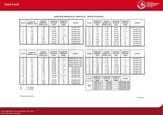
  • 38. RESULTADOS DE LA LÓGICA DE CONTROL Lecturas digitales del sensor analógico. Se aprecia que cada vez que transcurre un periodo de muestreo, el Arduino Mega genera un comando con la información recibida y lo envía a través de la comunicación serial hacia la Interfaz Gráfica del Usuario desarrollado en el software Labview 2012 de la empresa National Instruments.
  • 39. En este comando generado por el controlador, se puede observar que indica el número de sector en el cual se encuentra el proceso de riego. Posteriormente la lectura de los sensores que se encuentran distribuidos en tal sector, y por último, el estado lógico en el que se encuentra la válvula solenoide.
  • 40. Según la lógica de control del proceso de riego, este cambia de sector de riego si es que se supera el nivel de referencia de humedad de suelo. En este caso se estableció que el mencionado Set Point sea de 700, por tal razón se puede apreciar que una vez que supere el nivel indicado, la lógica de control cambia y realiza la acción de apagar la válvula con un estado lógico de ‘0’, esto se puede apreciar en el último comando generado en referencia al sector de riego 1. Luego se procede con la apertura de la válvula del segundo sector de riego, así sucesivamente hasta cubrir todo el terreno.
  • 42.
  • 43.
  • 44. INTERFAZ GRAFICA DE USUARIO Se presenta algunas imágenes que fueron tomadas mientras se realizaba las pruebas del diseño electrónico.
  • 45.
  • 46.
  • 47.
  • 48.
  • 49.
  • 50. Anexo 6 En el presente anexo se explica el diseño de la etapa de alimentación para la operación de la válvula solenoide. En el figura 1, se observa el circuito de simulación el cual consiste en una fuente de voltaje de corriente alterna (AC), configurada a 220 VAC y una frecuencia de 60 Hz. La siguiente etapa conformada por 4 diodos 1N4001 se conoce como rectificación de señal a onda completa, dicha etapa realiza la conversión de una señal AC a una señal DC. Por último, la resistencia R1 y el condensador C1 completan la conversión de la señal alterna disminuyendo el voltaje de rizado que se genera en la etapa de rectificación. Figura 1. Circuito de prueba En la figura anterior, se observa el circuito realizado en el software SpiceNet mediante el cual se puede analizar el voltaje de rizado que se genera en la punta de medición Y1. También se puede visualizar la señal de entrada de voltaje alterna V1 mediante la punta Y2, con el objetivo de asegurarse que la señal de entrada sea la correcta. 1 2 V1 2 2 1 1 1 3 D1 1N4001 2 3 D2 1N4001 2 D3 1N4001 1 D4 1N4001 1 1 1 1 1 1 3 C1 630u 3 3 3 3 3 3 1 1 1 1 1 1 1 1 2 2 2 2 2 2 2 2 3 Y1  + - 2 1 Y2 2 2 1 1 1 1 2 2 3 R1 32 3 3 3 3
  • 51. En la figura 2, se puede observar las gráficas generadas por la simulación del circuito desarrollado. Esto mediante la herramienta Scope del software SpiceNet. Figura 2. Gráficas de voltaje de entrada y salida del circuito de prueba.
  • 52. De la figura 2, se obtiene que la señal rectificada presente un voltaje de rizado de menor a un 1 voltio, aproximadamente 856 mV, lo cual es adecuado para diseños eléctricos ya que no supera el 5% del Voltaje pico de la señal. Sin embargo, dicho rango se encuentra fuera del rango de alimentación de la carga, en el presente trabajo de tesis se trata en una válvula solenoide; por esta razón, se requiere de una etapa que pueda brindar el suficiente voltaje como para alimentar la válvula solenoide, el cual consiste en adicionar un regulador de voltaje para que garantice el nivel de voltaje adecuado. Figura 3. Diseño del circuito de alimentación de la válvula solenoide. De esta forma, se realiza el diseño de alimentación de la electro – válvula tal y como se muestra en la figura 3; considerando su los efectos que se generan en la etapa de rectificación de una señal alterna, como también el rango de alimentación del actuador mecánico-eléctrico.
  • 53.
  • 54.
  • 55.
  • 56.
  • 57.
  • 58.
  • 59.
  • 60.
  • 61.
  • 62.
  • 63.
  • 64.
  • 65.
  • 66.
  • 67.
  • 68.
  • 69.
  • 70.
  • 71.
  • 72.
  • 73.
  • 74.
  • 75.
  • 76.
  • 77.
  • 78.
  • 79.
  • 80.
  • 81.
  • 82.
  • 83.
  • 84.
  • 85.
  • 86.
  • 87.
  • 88.
  • 89.
  • 90.
  • 91.
  • 92.
  • 93.
  • 94.
  • 95.
  • 96.
  • 97.
  • 98.
  • 99.
  • 100.
  • 101.
  • 102.
  • 103.
  • 104.
  • 105.
  • 106.
  • 107.
  • 108.
  • 109.
  • 110.
  • 111.
  • 112.
  • 113.
  • 114.
  • 115.
  • 116.
  • 117.
  • 118.
  • 119.
  • 120.
  • 121.
  • 122.
  • 123.
  • 124.
  • 125.
  • 126.
  • 127.
  • 128.
  • 129.
  • 130.
  • 131.
  • 132.
  • 133.
  • 134.
  • 135.
  • 136.
  • 137.
  • 138.
  • 139.
  • 140.
  • 141.
  • 142.
  • 143.
  • 144.
  • 145.
  • 146.
  • 147.
  • 148.
  • 149.
  • 150.
  • 151.
  • 152.
  • 153.
  • 154.
  • 155.
  • 156.
  • 157.
  • 158.
  • 159.
  • 160.
  • 161.
  • 162.
  • 163.
  • 164.
  • 165.
  • 166.
  • 167.
  • 168.
  • 169.
  • 170.
  • 171.
  • 172.
  • 173.
  • 174.
  • 175.
  • 176.
  • 177.
  • 178.
  • 179.
  • 180.
  • 181.
  • 182.
  • 183.
  • 184.
  • 185.
  • 186.
  • 187.
  • 188.
  • 189.
  • 190.
  • 191.
  • 192.
  • 193.
  • 194.
  • 195.
  • 196.
  • 197.
  • 198.
  • 199.
  • 200.
  • 201.
  • 202.
  • 203.
  • 204.
  • 205.
  • 206.
  • 207.
  • 208.
  • 209.
  • 210.
  • 211.
  • 212.
  • 213.
  • 214.
  • 215.
  • 216.
  • 217.
  • 218.
  • 219.
  • 220.
  • 221.
  • 222.
  • 223.
  • 224.
  • 225.
  • 226.
  • 227.
  • 228.
  • 229.
  • 230.
  • 231.
  • 232.
  • 233.
  • 234.
  • 235.
  • 236.
  • 237.
  • 238.
  • 239.
  • 240.
  • 241.
  • 242.
  • 243.
  • 244.
  • 245.
  • 246.
  • 247.
  • 248.
  • 249.
  • 250.
  • 251.
  • 252.
  • 253.
  • 254.
  • 255.
  • 256.
  • 257.
  • 258.
  • 259.
  • 260.
  • 261.
  • 262.
  • 263.
  • 264.
  • 265.
  • 266.
  • 267.
  • 268.
  • 269.
  • 270.
  • 271.
  • 272.
  • 273.
  • 274.
  • 275.
  • 276.
  • 277.
  • 278.
  • 279.
  • 280.
  • 281.
  • 282.
  • 283.
  • 284.
  • 285.
  • 286.
  • 287.
  • 288.
  • 289.
  • 290.
  • 291.
  • 292.
  • 293.
  • 294.
  • 295.
  • 296.
  • 297.
  • 298.
  • 299.
  • 300.
  • 301.
  • 302.
  • 303.
  • 304.
  • 305.
  • 306.
  • 307.
  • 308.
  • 309.
  • 310.
  • 311.
  • 312.
  • 313.
  • 314.
  • 315.
  • 316.
  • 317.
  • 318.
  • 319.
  • 320.
  • 321.
  • 322.
  • 323.
  • 324.
  • 325.
  • 326.
  • 327.
  • 328.
  • 329.
  • 330.
  • 331.
  • 332.
  • 333.
  • 334.
  • 335.
  • 336.
  • 337.
  • 338.
  • 339.
  • 340.
  • 341.
  • 342.
  • 343.
  • 344.
  • 345.
  • 346.
  • 347.
  • 348.
  • 349.
  • 350.
  • 351.
  • 352.
  • 353.
  • 354.
  • 355.
  • 356.
  • 357.
  • 358.
  • 359.
  • 360.
  • 361.
  • 362.
  • 363.
  • 364.
  • 365.
  • 366.
  • 367.
  • 368.
  • 369.
  • 370.
  • 371.
  • 372.
  • 373.
  • 374.
  • 375.
  • 376.
  • 377.
  • 378.
  • 379.
  • 380.
  • 381.
  • 382.
  • 383.
  • 384.
  • 385.
  • 386.
  • 387.
  • 388.
  • 389.
  • 390.
  • 391.
  • 392.
  • 393.
  • 394.
  • 395.
  • 396.
  • 397.
  • 398.
  • 399.
  • 400.
  • 401.
  • 402.
  • 403.
  • 404.
  • 405.
  • 406.
  • 407.
  • 408.
  • 409.
  • 410.
  • 411.
  • 412.
  • 413.
  • 414.
  • 415.
  • 416.
  • 417.
  • 418.
  • 419.
  • 420.
  • 421.
  • 422.
  • 423.
  • 424.
  • 425.
  • 426.
  • 427.
  • 428.
  • 429.
  • 430.
  • 431.
  • 432.
  • 433.
  • 434.
  • 435.
  • 436.
  • 437.
  • 438.
  • 439.
  • 440.
  • 441.
  • 442.
  • 443.
  • 444.
  • 445.
  • 446.
  • 447.
  • 448.
  • 449.
  • 450.
  • 451.
  • 452.
  • 453.
  • 454.
  • 455.
  • 456.
  • 457.
  • 458.
  • 459.
  • 460.
  • 461.
  • 462.
  • 463.
  • 464.
  • 465.
  • 466.
  • 467.
  • 468.
  • 469.
  • 470.
  • 471.
  • 472.
  • 473.
  • 474.
  • 475.
  • 476.
  • 477.
  • 478.
  • 479.
  • 480.
  • 481.
  • 482.
  • 483.
  • 484.
  • 485.
  • 486.
  • 487.
  • 488.
  • 489.
  • 490.
  • 491.
  • 492.
  • 493.
  • 494.
  • 495.
  • 496. ECH2O EA-10 Soil Moisture Sensor Integrator’s Guide Version 3
  • 497. Decagon Devices, Inc. All rights reserved ©2008-2011 Decagon Devices, Inc. 2365 NE Hopkins Court Pullman W A 99163 www.decagon.com
  • 498. EA-10 Soil Moisture Sensor Integrator’s Guide i Contents 1. Introduction . . . . . . . . . . . . . . 1 Specifications . . . . . . . . . . . . . . . . . . . . . . . . . . . . 1 Contact Information. . . . . . . . . . . . . . . . . . . . . . . 2 Warranty Information . . . . . . . . . . . . . . . . . . . . . 2 2. Installing the EA-10 . . . . . . . 4 Procedure . . . . . . . . . . . . . . . . . . . . . . . . . . . . . . . 4 Orientation. . . . . . . . . . . . . . . . . . . . . . . . . . 5 Turf Installation . . . . . . . . . . . . . . . . . . . . . . 5 Removing the Probe . . . . . . . . . . . . . . . . . . 6 Electrical Connection . . . . . . . . . . . . . . . . . . . . . 7 Hardware Requirements . . . . . . . . . . . . . . . . . . . 8 Troubleshooting . . . . . . . . . . . . . . . . . . . . . . . . . . 8 3. How the EA-10 Works . . . . 10 Calibration . . . . . . . . . . . . . . . . . . . . . . . . . . . . . . 11 Functional Testing . . . . . . . . . . . . . . . . . . . . . . . . 11 4. Further Reading . . . . . . . . 12 Index . . . . . . . . . . . . . . . . . . . . 13
  • 499. EA-10 Soil Moisture Sensor Integrator’s Guide 1. Introduction 1 1. Introduction Thank you for using the ECH2O EA-10 Dielectric Soil Moisture sensor. The EA-10 sensor has a stan- dard 2-wire, 4-20 mA analog interface for use with industrial data acquisition and control systems. Specifications Model: EA-10 Dielectric Soil Moisture Sensor. Electrical specs: Interface: 4-20 mA, 2-wire analog transmitter Red: (+) supply; Black: (-) supply; Shield: NC Supply voltage: line powered 7-32 Volt; DC Overvoltage and reverse polarity protected Sensor Specification: Measurement type: Volumetric Water Content (VWC) Measurement range: typical 0 to 40 percent VWC Measurement resolution: depends on acquisition hardware Measurement accuracy: ± 2% with soil specific calibra tion; accuracy at standard factory calibration varies depending on soil type Measurement output: current linearly related to VWC. Active sensor length: 10 cm Minimum measurement time: 10 ms Soils: all types; coarse sand to clay
  • 500. EA-10 Soil Moisture Sensor Integrator’s Guide 1. Introduction 2 Operating environment: Temperature: -40 to +50 °C. Humidity: 0-100% Physical properties: Dimensions: 14.5cm x 3.17cm x 0.15 cm Cable: 2 meter, 26 AWG tinned, bare wire (Custom length available upon request. Cost depends on length). Calibration: Percent Volumetric Water Content = 0.0425 x current (mA)-0.342 Functional testing: Sensor output in air: 4.0-5.5 mA Sensor output in water: 16.0-18.5 mA. Contact Information If you need to contact Decagon: • E-mail us at support@decagon.com • Send us a fax at (509) 332-5158 • Call us at: (US and Canada only) 1-800-755-2751 or 509-332-2756. Warranty Information The EA-10 has a 30-day satisfaction guarantee and a one-year warranty.
  • 501. EA-10 Soil Moisture Sensor Integrator’s Guide 1. Introduction 3 Seller’s Liability Seller warrants new equipment of its own manufacture against defective workmanship and materials for a period of one year from date of receipt of equipment (the results of ordinary wear and tear, neglect, misuse, accident and excessive deterioration due to corrosion from any cause are not to be considered a defect); but Seller’s liability for defective parts shall in no event exceed the furnishing of replacement parts F.O.B. the factory where originally manufactured. Material and equipment covered hereby which is not manufactured by Seller shall be covered only by the warranty of its manufacturer. Seller shall not be liable to Buyer for loss, damage or injuries to persons (including death), or to property or things of whatsoever kind (including, but not without limitation, loss of anticipated profits), occasioned by or arising out of the installation, opera- tion, use, misuse, nonuse, repair, or replacement of said material and equipment, or out of the use of any method or process for which the same may be employed. The use of this equipment constitutes Buyer’s acceptance of the terms set forth in this war- ranty. There are no understandings, representations, or warranties of any kind, express, implied, statutory or otherwise (including, but without limitation, the implied warranties of merchantability and fitness for a particular purpose), not expressly set forth herein.
  • 502. EA-10 Soil Moisture Sensor Integrator’s Guide 2. Installing the EA-10 4 2. Installing the EA-10 The EA-10 monitors the water content of the soil in which it is placed by measuring the dielectric constant of the soil and water surrounding the probe. While the probe measures just the soil which is adjacent to it, its reading is most useful if that measurement represents the general soil conditions in which the probe is placed. For that to happen, the monitoring site must be carefully selected, and the probe must be properly installed. Procedure When installing the EA-10 probe, it is best to maxi- mize contact between the probe and the soil. There are two methods to accomplish this. 1. Use Decagon’s Probe Installation Kit to install the probe. This kit has a custom-shaped blade to make the insertion in the soil, then another tool to place the probe into the insertion. For deeper installa- tions, use an augur to reach the desired depth, then use the Installation kit with extension rods to install the probe. 2. Use a thin implement like a trenching shovel, gar- dening spade, or flat bar to make a pilot hole in the soil. Then insert the probe into the hole, making sure the entire length of the probe is covered. Finally, insert the shovel again into the soil a few inches away from the probe, and gently force soil toward the probe to provide good contact
  • 503. at a 45° angle to the ground, instead of straight down. EA-10 Soil Moisture Sensor Integrator’s Guide 2. Installing the EA-10 5 between the probe and the soil. For deeper instal- lation, excavate down to the level you wish to mea- sure, then install the probe as described. When selecting a site for installation, it is important to remember that the soil adjacent to the probe surface has the strongest influence on the probe reading and that the probe measures the volumetric water content. Therefore any air gaps or excessive soil compaction around the probe can profoundly influence the read- ings. Also, do not install the probes adjacent to large metal objects such as metal poles or stakes. This can attenuate the probe’s electromagnetic field and adversely affect output readings. Orientation The probe can be oriented in any direction. However, orienting the flat side perpendicular to the surface of the soil will minimize effects on downward water movement. Turf Installation When installing the EA-10, the installation procedure is almost the same, except that the probe is ofteplaced
  • 504. break internal connections and make the probe unus- EA-10 Soil Moisture Sensor Integrator’s Guide 2. Installing the EA-10 6 Removing the Probe When removing the probe from the soil, do not pull it out of the soil by the cable! Doing so may able. 45° 1.0" Ground Level
  • 505. EA-10 Soil Moisture Sensor Integrator’s Guide 2. Installing the EA-10 7 Electrical Connection The EA-10 is a 2 wire, 4 - 20 mA transmitter. When connected to a 7 - 32 volt source (line power), the cur- rent is linearly proportional to the water content of the soil. The red wire is connected to the positive terminal and the black wire is the return for the negative terminal. The shield (bare wire) can be connected to a shield terminal, if available, or left open. The probe is electri- ECH2 O EA-10 Soi lM oi sture Sensor •4-20 m A transm i tter Patent 6904789 R1-05 DECAGON DEVICES www.decagon.com ® 7 to 36 Volt DC Source Red Wire Black Wire Current Sense Circuit 4–20 mA Analog Hardware Shield Wire to Ground
  • 506. EA-10 Soil Moisture Sensor Integrator’s Guide 2. Installing the EA-10 8 cally floating, and the shield is not electrically con- nected to the probe circuitry. Extension wire can be used to connect the EA-10 to the 4-20 mA receiver. The extension wire should be a 2 conductor shielded, direct burial cable. NOTE: It is essential that sensor wire connec- tions be watertight! Use wire nuts with grease or silicon gel caps for all splices. Hardware Requirements The EA-10 is designed to work with industrial control and acquisition devices. The EA-10 is loop powered, drawing its operational power from the current used to measure volumetric water content. Any device capable of producing a 7 - 32 mA loop voltage should be compatible with the EA-10. The EA-10 is also reverse-polarity protected. If it is installed in the wrong direction, it will not operate, but will be pro- tected from electrical overload. NOTE: The EA-10 is intended for use with indus- trial control and acquisition devices which can provide a short pulse, leaving the probes turned off most of the time. Continuous power may cause the probe to exceed government FCC limits on electromagnetic emissions.
  • 507. EA-10 Soil Moisture Sensor Integrator’s Guide 2. Installing the EA-10 9 Troubleshooting If you encounter problems with the EA-10, they will usually be in the form of negative or erroneous VWC readings. The most common solution to this problem is to make sure that you have adequate probe-to-soil contact. When inserted, the EA-10 should be com- pletely covered up to the black overmolding. Doing this should remedy any reading errors. If it does not, please contact Decagon for assistance.
  • 508. EA-10 Soil Moisture Sensor Integrator’s Guide 3. How the EA-10 Works 10 3. How the EA-10 Works In essence, the EA-10 monitors the water budget of the soil in which it is placed. It senses water addition and water loss. If the soil is too wet, irrigation can be stopped. If the soil becomes too dry, additional irriga- tion time can be programmed. Proper monitoring of the water budget requires that the moisture sensor be located in the active root zone of relatively homogeneous vegetation, and in well- drained soil of above-average moisture holding capac- ity. Avoid locations where water can run-on or pool, and locations with poor vegetative cover, or where vegetation tends to water stress because of poor mois- ture holding capacity of the soil or shallow root zone. Vegetation in non-monitored zones will use water at a rate proportional to water use in the monitored zone. Water application rates in these zones must therefore be proportional for the entire system to remain prop- erly irrigated. If trees use 30% more water than turf, and turf is being monitored, then the tree zone needs to be irrigated for 30% more time than the monitored turf to maintain adequate soil moisture. Since dielectric probes (such as the EA-10) measure the moisture in the immediate vicinity of the probe, it is essential that the probe be installed so that the entire length of the probe is in intimate contact with the soil
  • 509. EA-10 Soil Moisture Sensor Integrator’s Guide 3. How the EA-10 Works 11 (no air gaps). The soil must therefore be packed tightly around the entire probe length during installation. The probe is installed with the blade perpendicular to the surface to interfere as little as possible with water movement through the soil. Calibration The probe reading is converted to volumetric water content using the following equation: Volumetric Water Content = 0.0425 x Current (mA)- 0.342 Water content is in m3 m-3 , and current is in milli- amps. For water content in terms of percent of total volume, use the following equation: Volume percent = 4.25 x Current - 34.2. These calibrations are for typical soils with mid range texture, and are accurate enough for most irrigation scheduling purposes. For greater accuracy, a soil spe- cific calibration should be undertaken, as outlined on the Decagon website. Functional Testing ECH2O EA-10 sensors are tested to perform cor- rectly in the following conditions: Sensor output in air: 4.0-5.5 mA Sensor output in distilled water: 16.0-18.5mA
  • 510. EA-10 Soil Moisture Sensor Integrator’s Guide 4. Further Reading 12 4. Further Reading ECH2O Probes Soil-Specific Calibration http://www.decagon.com/ag_research/literature/ app_notes.php ECH2O Dielectric Probes vs. Time Domain Reflectometers (TDR) http://www.decagon.com/ag_research/literature/ app_notes.php ECH2O Probe insertion guide http://www.decagon.com/ag_research/literature/ app_notes.php
  • 511. EA-10 Soil Moisture Sensor Integrator’s Guide Index 13 Index C Calibration 11 Contact information 2 F Functional testing 11 I Installation electrical connection 7 hardware requirements 8 procedure 4 S Seller’s Liability 2 Specifications 1 T Troubleshooting 8 W Warranty 2
  • 512. Electroválvulas servoaccionadas de 2/2 vías Modelo EV220B DN 6-22 DKACV.PD.200.C3.05 520B1636 Mayo 2003 Especificaciones técnicas
  • 513. DKACV.PD.200.C3.05 Danfoss A/S 05-2003 2 1 /4 - 1” NPT • Para aplicaciones industriales severas • Para agua, aceite, aire comprimido y fluidos neutros similares • Rango de caudal de agua: 0,2 - 19 m3/h • Presión diferencial: Hasta 30 bar • Viscosidad: Hasta 50 cSt • Temperatura ambiente: Hasta 80°C • Protección de la bobina: Hasta IP 67 • Conexiones de la rosca: Desde 1 /4 hasta 1” NPT • Disponible también con rosca G. Por favor, póngase en contacto con Danfoss. • Versiones NC en EPDM con aprobación WRAS Dimensiones y peso Opciones de la bobina Válvula servoaccionada de 2/2 vías Modelo EV220B para líquidos y gases neutros DN 6 -22 B Desactivada cerrada Características Datos técnicos 1 ) Los tiempos son indicativos y se aplican para agua. Los tiempos exactos dependerán de las condiciones de presión. Modelo EV220B 6 B EV220B 10 B EV220B 12 B EV220B 18B EV220B 22B Instalación Serecomiendaunsistema deelectroválvulasvertical (véaseDKACV.PT.600.A) Rango de presión 0.1 - 30 bar Max. presión de prueba EV220B 6 -10 B: 50 bar. EV220B 12-22 B: 16 bar Tiempo de apertura 1 ) 40 ms 50 ms 60 ms 200 ms 200 ms Tiempo de cierre 1 ) 250 ms 300 ms 300 ms 500 ms 500 ms Temperatura ambeiente 40 - 80°C (dependiendo del mod. de bobina, véanse los datos de la bobina seleccionada) Temperatura del fluido EPDM: -30 a + 100°C. FKM: De 0 a + 100°C Viscosidad max. 50 cSt Materiales Cuerpo de la válvula: Latón, n o . 2.0402 Armadura: Acero inoxidable n o . 1.4105/AISI 430FR Tubo de la armadura: Acero inoxidable n o . 1.4306/AISI 304L Tope de la armadura: Acero inoxidable n o . 1.4105/AISI 430FR Muelles: Acero inoxidable n o . 1.4310/AISI 301 Juntas tóricas: EPDM o FKM Clapet: EPDM o FKM Diafragma: EPDM o FKM Modelo: BA 9 W ca 15 W cc Modelo:BB 10 W ca 18W cc Modelo: BE (IP67) 10 W ca 18 W cc Modelo: BG 12 W ac 20 W dc Danfoss dispone de bobinas exentas de ruidos para aplicaciones sensibles a los mismos, y también de bobinas EEx m II T4 para su utilización en áreas con riesgo de explosión - para más información consulte la hoja dedatosDKACV.PD.600.A Véase DKACV.PD.600.A Modelo L B B 1 [mm] H1 H Peso Modelodebobina Modelodebobina Modelodebobina sin bobina [mm] [mm] BA/BD BB/BE BG [mm] [mm] [kg] EV220B 6B 45.5 43.5 32 46 68 13.0 74.0 0.22 EV220B 10B 51.5 48.0 32 46 68 13.0 77.0 0.29 EV220B 12B 58.0 54.0 32 46 68 13.0 77.0 0.35 EV220B 18B 90.0 62.0 32 46 68 18.0 83.0 0.65 EV220B 22B 90.0 62.0 32 46 68 18.0 98.0 0.65
  • 514. DKACV.PD.200.C3.05-NPT Danfoss A/S 05-2003 3 Desactivada cerrada 1 /4 “- 1” NPT Función Tensión de bobina desconectada (cerrada): Cuando la tensión de la bobina (8) está desconectada, el muelle de la armadura (1) presiona el clapet (3) contra el orificio del piloto (6). La presión a lo largo del diafragma (7) se crea mediante el orificio de compensación (4). El diafragma cierra el orificio principal (5) tan pronto como la presión del diafragma es equivalente a la presión de entrada. La válvula permanecerá cerrada mientras la tensión de la bobina esté desconectada. Tensión de la bobina conectada (abierta): Cuando se aplica tensión a la bobina, se abre el orificio piloto (6). Como el orificio piloto es mayor que el orificio de compensación (4), la presión a lo largo del diafragma (7) cae y así se eleva libre del orificio principal (5). Ahora la válvula está abierta y permanecerá así mientras se mantenga la presión diferencial mínima a lo largo de la válvula y mientras se aplique tensión a la válvula. 1. Muelle de la armadura 2. Armadura 3. Clapet 4. Orificio de compensación 5. Orificio principal 6. Orificio piloto 7. Diafragma 8. Bobina Pedidos: cuerpo de la válvula Válvula servoaccionada de 2/2 vías Modelo EV220B para líquidos y gases neutros DN 6 -22 B 1 ) Indicado sólo para agua. 2 ) Indicado para aceite y aire. También se puede utilizar para agua y soluciones acuosas neutras siempre y cuando la temperatura del agua no exceda de 60 °C. = sólo gas Pedidos: bobinas Véase en las especificaciones técnicas separadas las bobinas DKACV.PD.600.A Conexión Material Valor Temp. Codigo de Presióndiferencialpermisible[bar]/Modelodebobina de junta k v de fluido Selección del modelo bobina Min. Max. NPT [m3 /h] A B . x á M . n i M BB/BE BG [°C] [°C] Modelo principal Especificación Standard) 9 W 15 W 10 W 18 W 12 W 20 W ca cc ca cc ca cc 3 /8 EPDM 1 ) 0.7 -30 +100 EV220B 6 B N 38E NC000 032U7514 0.1 20 - 20 10 20 20 3 /8 FKM 2 ) 0.7 0 +100 EV220B 6 B N 38F NC000 032U7516 0.1 20 - 20 10 20 20 0.1 30 - 30 - 30 30 3 /8 EPDM 1 ) 1.5 -30 +100 EV220B 10 B N 38E NC000 032U7517 0.1 20 - 20 10 20 20 3/8 FKM 2 ) 1.5 0 +100 EV220B 10 B N 38F NC000 032U7519 0.1 20 - 20 10 20 20 0.1 30 - 30 - 30 30 1/2 EPDM 1 ) 1.5 -30 +100 EV220B 10 B N 12E NC000 032U7518 0.1 20 - 20 10 20 20 1 /2 FKM 2 ) 1.5 0 +100 EV220B 10 B N 12F NC000 032U7520 0.1 20 - 20 10 20 20 0.1 30 - 30 - 30 30 1 /2 EPDM 1 ) 2.5 -30 +100 EV220B 12 B N 12E NC000 032U7521 0.3 10 - 10 - - 10 1 /2 FKM 2 ) 2.5 0 +100 EV220B 12 B N 12F NC000 032U7522 0.3 10 - 10 - - 10 3 /4 EPDM 1 ) 6.0 -30 +100 EV220B 18B N 34E NC000 032U7523 0.3 10 - 10 - 10 10 3/4 FKM 2) 6.0 0 +100 EV220B 18B N 34F NC000 032U7524 0.3 10 - 10 - 10 10 1 EPDM 1) 6.0 -30 +100 EV220B 22B N 1E NC000 032U7525 0.3 10 - 10 - 10 10 1 FKM2) 6.0 0 +100 EV220B 22B N 1F NC000 032U7526 0.3 10 - 10 - 10 10
  • 515. DKACV.PD.200.C3.05 Danfoss A/S 05-2003 4 G 3 /8 G 1 /2 Instalación Se recomienda un sistema de electroválvulas vertical, véase DKACV.PT.600.A Rango de presión 0,1 - 10 bar Máx. presión de prueba 50 bar Tiempo de apertura 1 ) EV220 6 B: 40 ms EV220 10 B: 50 ms Tiempo de cierre 1 ) EV220 6 B: 250 ms EV220 10 B: 300 ms Temperatura ambiente máx. 80°C (dependiendo del mod. de bobina, véanse los datos de la bobina seleccionada) Temperatura del fluido EPDM: -30 +100 °C. FKM: 0 - +100 °C Viscosidad máx. 50 cSt Materiales Cuerpo de la válvula: Latón, nº 2.0402 Armadura: Acero inoxidable nº 1.4105/AISI 430FR Tubo de la armadura: Acero inoxidable nº 1.4306/AISI 430FR Tope de la armadura: Acero inoxidable nº 1.4105/AISI 430FR Muelles: Acero inoxidable nº 1.4310/AISI 301 Juntas tóricas: EPDM o FKM Clapet: EPDM o FKM Diafragma: EPDM o FKM • Para aplicaciones industriales severas • Para agua, aceite, aire comprimido y fluidos neutros similares • Rango de caudal de agua: 0,2 - 3,15 m3/h • Presión diferencial: Hasta 10 bar • Viscosidad: Hasta 50 cSt • Temperatura ambiente: Hasta 80°C • Protección de la bobina: Hasta IP 67 • Conexiones de la rosca: G 3 /8 y G 1 /2 • Golpe de ariete amortiguado • Disponible también con rosca NPT. Por favor, póngase en contacto con Danfoss. Opciones de la bobina Dimensiones y peso Válvula servoaccionada de 2/2 vías Modelo EV220B NO (solo en version con conexion G) para líquidos y gases neutros DN 6 -10 B 1 ) Los tiempos son indicativos y se aplican para agua. Los tiempos exactos dependerán de las condiciones de presión y de trabajo. Desactivada abierta Características Datos técnicos Modelo L B B 1 [mm] H 1 H Peso [mm] [mm] Modelo de bobina Modelo de bobina [mm] [mm] sin bobina BA BB/BE [kg] EV220B 6 B NO 45,5 43,5 32 46 13 79 0,22 EV220B 10 B NO 51,0 48,0 32 46 13 82 0.29 Modelo: BB 10 W ca 18 W cc Modelo: BA 9 W ca 15 W cc Modelo: BE (IP67) 10 W ca 18 W cc Véase DKACV.PD.600.A Danfoss dispone én de bobinas exentas de ruidos para aplicaciones sensibles a los mismos, y también de bobinas EEx m II T4 para su utilización en áreas con riesgo de explosión - para más información consulte la hoja de datos DKACV.PD.600.A
  • 516. DKACV.PD.200.C3.05  Danfoss A/S 05-2003 5 G 3 /8 G 1 /2 Función Tensión de bobina desconectada (abierta): Cuando se desconecta la tensión de la bobina, se abre el orificio piloto (6). Como el orificio piloto es mayor que el orificio de compensación (4), la presión a lo largo del diafragma (7) cae y así se eleva libre del orificio principal (5). La válvula permanecerá abierta mientras se mantenga la presión diferencial mínima a lo largo de la válvula y mientras la tensión de la bobina esté desconectada. Tensión de bobina conectada (cerrada): Cuando se aplica tensión a la bobina, el clapet (3) es presionado contra el orificio piloto (6). La presión a lo largo del diafragma (7) se crea mediante el orificio de compensación (4). El diafragma cierra el orificio principal (5) tan pronto como la presión del diafragma es equivalente a la presión de entrada. La válvula permanecerá cerrada mientras la tensión de la bobina esté conectada. Pedidos: cuerpo de la válvula Desactivada abierta 1. Muelle de apertura 2. Armadura 3. Clapet 4. Orificio de compensación 5. Orificio principal 6. Orificio piloto 7. Diafragma 8. Bobina Válvula servoaccionada de 2/2 vías Modelo EV220B NO para líquidos y gases neutros DN 6 -10 B 1 ) Indicado sólo para agua. 2 ) Indicado para aceite y aire. También se puede utilizar para agua y soluciones acuosas neutras siempre y cuando la temperatura del agua no exceda de 60 °C. Pedidos: bobinas Véase en las especificaciones técnicas separadas las bobinas DKACV.PD.600.A Connec- Joint kv- Fluide Nº de code Pression diff. admissible (bar) tion matériaux valeur temp. Désignation du modèle sans Min. Máx. ISO [m3/h] Mín. Máx. bobine BA BB BE 228/1 [°C] [°C] Type principal Spécification 9 W 15 W 10 W 18 W 10W 18 W ca cc ca cc ca cc G 3/8 EPDM1 ) 0.7 -30 +100 EV220B 6 B G 38E NO000 032U1238 0,1 10 10 10 10 10 10 G 3/8 FKM2 ) 0,7 0 +100 EV220B 6 B G 38F NO000 032U1239 0,1 10 10 10 10 10 10 G 1 /2 FKM2 ) 1,0 0 +100 EV220B 10 B G 12F NO000 032U1249 0,1 10 10 10 10 10 10 Mín. Presión diferencial admisible [bar]/Modelo de bobina Código de bobina Modelo principal Especificación Valor kv [m3 /h] Material de junta Conexión ISO228/1 Selección del modelo Temp. de fluido
  • 517. DKACV.PD.200.C3.05  Danfoss A/S 05-2003 6 Válvula servoaccionada de 2/2 vías Modelo EV220B para líquidos y gases ligeramente agresivos DN 6 -12 BD (Latón resistente a la descincación) G 1 /4 - G 1 /2 • Para aplicaciones industriales severas • Para gases y líquidos ligeramente agresivos y neutros. Póngase en contacto con Danfoss si tuviera alguna duda sobre la adaptabilidad de la válvula al fluido en cuestión. • Presión diferencial: Hasta 20 bar • Viscosidad: Hasta 50 cSt • Temperatura ambiente: Hasta 80°C • Protección de la bobina: Hasta IP 67 • Conexiones de la rosca: Desde G 1 /4 hasta G 1 /2 Modelo EV220B 6 BD EV220B 10 BD EV220B 12 BD Instalación Se recomienda un sistema de electroválvulas vertical (véase DKACV.PT.600.A) Rango de presión 0,1 - 20 bar Máx. presión de prueba 50 bar 50 bar 16 bar Tiempo de apertura1 ) 40 ms 50 ms 60 ms Tiempo de cierre1 ) 250 ms 300 ms 300 ms Temperatura ambiente 40 - 80°C (dependiendo del modelo de bobina, véanse los datos de la bobina seleccionada) Temperatura del fluido −10 a +90°C Viscosidad máx. 50 cSt Materiales Cuerpo de la válvula: Latón resistente a la descincación: CuZn36Pb2As/CZ132 Armadura: Acero inoxidable, Nº 1.4105/AISI 430FR Tubo de la armadura: Acero inoxidable, Nº 1.4306/AISI 304L Tope de la armadura: Acero inoxidable, Nº 1.4105/AISI 430FR Muelles: Acero inoxidable, Nº 1.4310/AISI 301 Asiento de la válvula: Acero inoxidable, nº 1.4404/AISI 316L Juntas tóricas: EPDM Clapet: EPDM Diafragma: EPDM Dimensiones y peso Modelo L B B 1 [mm] H1 H Peso [mm] [mm] Modelo de bobinaModelo de bobinaModelo de bobina [mm] [mm] sin bobina BA BB/BE BG [kg] EV220B 6 BD 45,5 43,5 32 46 68 13,0 74,0 0,22 EV220B 10 BD 51,0 48,0 32 46 68 13,0 77,0 0,29 EV220B 12 BD 58,0 50,0 32 46 68 13,0 77,0 0,35 Opciones de la bobina 1 ) Los tiempos son indicativos y se aplican para agua. Los tiempos exactos dependerán de las condiciones de presión. Desactivada cerrada Características Datos técnicos Modelo: BA 9 W ca 15 W cc Modelo:BB 10 W ca 18W cc Modelo: BE (IP67) 10 W ca 18 W cc Modelo: BG 12 W ac 20 W dc Danfoss dispone én de bobinas exentas de ruidos para aplicaciones sensibles a los mismos, y también de bobinas EEx m II T4 para su utili- zación en áreas con riesgo de explosión - para más información consulte la hoja de datos DKACV.PD.600.A Véase DKACV.PD.600.A
  • 518. DKACV.PD.200.C3.05  Danfoss A/S 05-2003 7 Válvula servoaccionada de 2/2 vías Modelo EV220B para líquidos y gases ligeramente agresivos DN 6 -12 BD (Latón resistente a la descincación) Desactivada cerrada G 1 /4 - G 1 /2 Tensión de bobina desconectada (cerrada): Cuando la tensión de la bobina (8) está desconectada, el muelle de cierre (1) presiona el clapet (3) contra el orificio piloto (6). La presión a lo largo del diafragma (7) se crea mediante el orificio de compensación (4). El diafragma cierra el orificio principal (5) tan pronto como la presión del diafragma es equivalente a la presión de entrada. La válvula permanecerá cerrada mientras la tensión de la bobina esté desconectada. 1. Muelle de cierre 2. Armadura 3. Clapet 4. Orificio de compensación 5. Orificio principal 6. Orificio piloto 7. Diafragma 8. Bobina Función Pedidos: cuerpo de la válvula Tensión de la bobina conectada (abierta): Cuando se aplica tensión a la bobina, se abre el orificio piloto (6). Como el orificio piloto es mayor que el orificio de compensación (4), la presión a lo largo del diafragma (7) cae y así se eleva libre del orificio principal (5). Ahora la válvula está abierta y permanecerá así mientras se mantenga la presión diferencial mínima a lo largo de la válvula y mientras se aplique tensión a la válvula. Pedidos: bobinas Véase en las especificaciones técnicas separadas las bobinas DKACV.PD.600.A Connec- Joint kv- Fluide Nº de code Presión diferencial admisible [bar] tion matériauxvaleur temp. Désignation du modèle sMín. Máx. ISO [m3/h] Mín. Máx. bobine BA BB BE 228/1 [°C] [°C] Type principal Spécification 9 W 15 W 10 W 18 W 12 W 20 W ca cc ca cc ca cc G 1 /4 EPDM1 ) 0,7 -30 +100 EV 220B 6 BD G 14E NC000 032U5806 0,1 20 - 20 10 20 20 G 3 /8 EPDM1 ) 0,7 -30 +100 EV 220B 6 BD G 38E NC000 032U5807 0,1 20 - 20 10 20 20 G 3 /8 EPDM1 ) 1,5 -30 +100 EV 220B 10 BD G 38E NC000 032U5809 0,1 20 - 20 10 20 20 G 1 /2 EPDM1 ) 1,5 -30 +100 EV 220B 10 BD G 12E NC000 032U5810 0,1 20 - 20 10 20 20 G 1 /2 EPDM1 ) 2,5 -30 +100 EV 220B 12 BD G 12E NC000 032U5811 0,3 10 - 10 - - 10 Modelo principal Especificación Código de bobina Valor kv [m3/h] Material de junta Conexión ISO228/1 Selección del modelo Temp. de fluido 1 ) Indicado sólo para agua.
  • 519. DKACV.PD.200.C3.05  Danfoss A/S 05-2003 8 Kit de repuestos para electroválvulas servoaccionadas de 2/2 vías Modelo EV220B Kit de repuestos - EV220B 6-22 B: (cuerpo de latón) - EV220B 6 - 12 BD (cuerpo de latón resistente a la descincación) El kit de piezas de recambio contiene un botón de bloqueo, una tuerca para la bobina, armadura con clapet y muelle, y un diafragma. Para EV220B6 y 10, el kit de repuestos también incluye una junta tórica. Modelo Material Código junta Estándar WRAS EV220B 6 B EPDM1 ) 032U1062 032U6001 EV220B 6 B FKM2 ) 032U1063 EV220B 10 B EPDM1 ) 032U1065 032U6002 EV220B 10 B FKM2 ) 032U1066 EV220B 12 B EPDM1 ) 032U1068 032U6003 EV220B 12 B FKM2 ) 032U1067 EV220B18-22 EPDM1 ) 032U1070 032U6004 EV220B18-22 FKM2 ) 032U1069 Modelo Material Código junta EV220B 6 BD EPDM1 ) 032U4280 EV220B 10 BD EPDM1 ) 032U4281 EV220B 12 BD EPDM1 ) 032U4282 Unidad de ensamblaje normalmente abierta (NO) EV220B 6 -10 B, NO Modelo Material Código junta DN 6 EPDM1 ) 032U0165 DN 6 FKM2 ) 032U0166 DN 10 FKM2 ) 032U0167 1 ) Indicado para agua. 2 ) Indicado para aceite y aire. Para agua temp. máx. 60 °C IC-MC/frz
  • 520. 1/13 ■ WIDE GAIN BANDWIDTH : 1.3MHz ■ INPUT COMMON-MODE VOLTAGE RANGE INCLUDES GROUND ■ LARGE VOLTAGE GAIN : 100dB ■ VERY LOW SUPPLY CURRENT/AMPLI : 375µA ■ LOW INPUT BIAS CURRENT : 20nA ■ LOW INPUT OFFSET VOLTAGE : 5mV max. (for more accurate applications, use the equiv- alent parts LM124A-LM224A-LM324A which feature 3mV max.) ■ LOW INPUT OFFSET CURRENT : 2nA ■ WIDE POWER SUPPLY RANGE : SINGLE SUPPLY : +3V TO +30V DUAL SUPPLIES : ±1.5V TO ±15V DESCRIPTION These circuits consist of four independent, high gain, internally frequency compensated operation- al amplifiers. They operate from a single power supply over a wide range of voltages. Operation from split power supplies is also possible and the low power supply current drain is independent of the magnitude of the power supply voltage. ORDER CODE N = Dual in Line Package (DIP) D = Small Outline Package (SO) - also available in Tape & Reel (DT) P = Thin Shrink Small Outline Package (TSSOP) - only available in Tape &Reel (PT) PIN CONNECTIONS (top view) Part Number Temperature Range Package N D P LM124 -55°C, +125°C • • • LM224 -40°C, +105°C • • • LM324 0°C, +70°C • • • Example : LM224N N DIP14 (Plastic Package) D SO14 (Plastic Micropackage) P TSSOP14 (Thin Shrink Small Outline Package) Inverting Input 2 Non-inverting Input 2 Non-inverting Input 1 CC V - CC V 1 2 3 4 8 5 6 7 9 10 11 12 13 14 + Output 3 Output 4 Non-inverting Input 4 Inverting Input 4 Non-inverting Input 3 Inverting Input 3 - + - + - + - + Output 1 Inverting Input 1 Output 2 LM124 LM224 - LM324 LOW POWER QUAD OPERATIONAL AMPLIFIERS December 2001
  • 521. LM124-LM224-LM324 2/13 SCHEMATIC DIAGRAM (1/4 LM124) ABSOLUTE MAXIMUM RATINGS Symbol Parameter LM124 LM224 LM324 Unit VCC Supply voltage ±16 or 32 V Vi Input Voltage -0.3 to +32 V Vid Differential Input Voltage 1) 1. Either or both input voltages must not exceed the magnitude of VCC + or VCC -. +32 V Ptot Power Dissipation N Suffix D Suffix 500 500 400 500 400 mW mW Output Short-circuit Duration 2) 2. Short-circuits from the output to VCC can cause excessive heating if VCC > 15V. The maximum output current is approximately 40mA independent of the magnitude of VCC. Destructive dissipation can result from simultaneous short-circuit on all amplifiers. Infinite Iin Input Current 3) 3. This input current only exists when the voltage at any of the input leads is driven negative. It is due to the collector-base junction of the input PNP transistor becoming forward biased and thereby acting as input diodes clamps. In addition to this diode action, there is also NPN parasitic action on the IC chip. this transistor action can cause the output voltages of the Op-amps to go to the VCC voltage level (or to ground for a large overdrive) for the time duration than an input is driven negative. This is not destructive and normal output will set up again for input voltage higher than -0.3V. 50 50 50 mA Toper Opearting Free-air Temperature Range -55 to +125 -40 to +105 0 to +70 °C Tstg Storage Temperature Range -65 to +150 °C
  • 522. LM124-LM224-LM324 3/13 ELECTRICAL CHARACTERISTICS VCC + = +5V, VCC - = Ground, Vo = 1.4V, Tamb = +25°C (unless otherwise specified) Symbol Parameter Min. Typ. Max. Unit Vio Input Offset Voltage - note 1) Tamb = +25°C LM324 Tmin ≤ Tamb ≤ Tmax LM324 2 5 7 7 9 mV Iio Input Offset Current Tamb = +25°C Tmin ≤ Tamb ≤ Tmax 2 30 100 nA Iib Input Bias Current - note 2) Tamb = +25°C Tmin ≤ Tamb ≤ Tmax 20 150 300 nA Avd Large Signal Voltage Gain VCC + = +15V, RL = 2kΩ, Vo = 1.4V to 11.4V Tamb = +25°C Tmin ≤ Tamb ≤ Tmax 50 25 100 V/mV SVR Supply Voltage Rejection Ratio (Rs ≤ 10kΩ) VCC + = 5V to 30V Tamb = +25°C Tmin ≤ Tamb ≤ Tmax 65 65 110 dB ICC Supply Current, all Amp, no load Tamb = +25°C VCC = +5V VCC = +30V Tmin ≤ Tamb ≤ Tmax VCC = +5V VCC = +30V 0.7 1.5 0.8 1.5 1.2 3 1.2 3 mA Vicm Input Common Mode Voltage Range VCC = +30V - note 3) Tamb = +25°C Tmin ≤ Tamb ≤ Tmax 0 0 VCC -1.5 VCC -2 V CMR Common Mode Rejection Ratio (Rs ≤ 10kΩ) Tamb = +25°C Tmin ≤ Tamb ≤ Tmax 70 60 80 dB Isource Output Current Source (Vid = +1V) VCC = +15V, Vo = +2V 20 40 70 mA Isink Output Sink Current (Vid = -1V) VCC = +15V, Vo = +2V VCC = +15V, Vo = +0.2V 10 12 20 50 mA µA VOH High Level Output Voltage VCC = +30V Tamb = +25°C RL = 2kΩ Tmin ≤ Tamb ≤ Tmax Tamb = +25°C RL = 10kΩ Tmin ≤ Tamb ≤ Tmax VCC = +5V, RL = 2kΩ Tamb = +25°C Tmin ≤ Tamb ≤ Tmax 26 26 27 27 3.5 3 27 28 V
  • 523. LM124-LM224-LM324 4/13 VOL Low Level Output Voltage (RL = 10kΩ) Tamb = +25°C Tmin ≤ Tamb ≤ Tmax 5 20 20 mV SR Slew Rate VCC = 15V, Vi = 0.5 to 3V, RL = 2kΩ, CL = 100pF, unity Gain 0.4 V/µs GBP Gain Bandwidth Product VCC = 30V, f =100kHz,Vin = 10mV, RL = 2kΩ, CL = 100pF 1.3 MHz THD Total Harmonic Distortion f = 1kHz, Av = 20dB, RL = 2kΩ, Vo = 2Vpp, CL = 100pF, VCC = 30V 0.015 % en Equivalent Input Noise Voltage f = 1kHz, Rs = 100Ω, VCC = 30V 40 DVio Input Offset Voltage Drift 7 30 µV/°C DIIio Input Offset Current Drift 10 200 pA/°C Vo1/Vo2 Channel Separation - note 4) 1kHz ≤ f ≤ 20kHZ 120 dB 1. Vo = 1.4V, Rs = 0Ω, 5V < VCC + < 30V, 0 < Vic < VCC + - 1.5V 2. The direction of the input current is out of the IC. This current is essentially constant, independent of the state of the output so no loading change exists on the input lines. 3. The input common-mode voltage of either input signal voltage should not be allowed to go negative by more than 0.3V. The upper end of the common-mode voltage range is VCC + - 1.5V, but either or both inputs can go to +32V without damage. 4. Due to the proximity of external components insure that coupling is not originating via stray capacitance between these external parts. This typically can be detected as this type of capacitance increases at higher frequences. Symbol Parameter Min. Typ. Max. Unit nV Hz ----------- -
  • 526. LM124-LM224-LM324 7/13 TYPICAL SINGLE - SUPPLY APPLICATIONS AC COUPLED INVERTING AMPLIFIER AC COUPLED NON INVERTING AMPLIFIER 1/4 LM124 ~ 0 2V PP R 10kW L Co eo R 6.2kW B R 100kW f R1 10kW CI eI V CC R2 100kW C1 10m F R3 100kW A = - R R1 V f (as shown A = -10) V 1/4 LM124 ~ 0 2V PP R 10kW L Co eo R 6.2kW B C1 0.1m F eI V CC (as shown A = 11) V A = 1 +R2 R1 V R1 100kW R2 1MW CI R3 1MW R4 100kW R5 100kW C2 10m F
  • 527. LM124-LM224-LM324 8/13 TYPICAL SINGLE - SUPPLY APPLICATIONS NON-INVERTING DC GAIN HIGH INPUT Z ADJUSTABLE GAIN DC INSTRUMENTATION AMPLIFIER DC SUMMING AMPLIFIER LOW DRIFT PEAK DETECTOR R1 10kW R2 1MW 1/4 LM124 10kW eI eO +5V e O (V) (mV) 0 AV= 1 + R2 R1 (As shown = 101) AV 1/4 LM124 R3 100kW eO 1/4 LM124 R1 100kW e1 1/4 LM124 R7 100kW R6 100kW R5 100kW e2 R2 2kW Gain adjust R4 100kW if R1 = R5 and R3 = R4 = R6 = R7 e0 = (e2 -e1) As shown e0 = 101 (e2 - e1). 1 2R 1 R 2 ---------- - + 1/4 LM124 eO e 4 e 3 e 2 e 1 100kW 100kW 100kW 100kW 100kW 100kW e0 = e1 +e2 -e3 -e4 Where (e1 +e2) ≥ (e3 +e4) to keep e0 ≥ 0V IB 2N 929 0.001m F IB 3R 3MW IB Input current compensation eo IB e I 1/4 LM124 Zo ZI C 1m F 2IB R 1MW 2IB * Polycarbonate or polyethylene * 1/4 LM124 1/4 LM124
  • 528. LM124-LM224-LM324 9/13 TYPICAL SINGLE - SUPPLY APPLICATIONS ACTIVER BANDPASS FILTER HIGH INPUT Z, DC DIFFERENTIAL AMPLIFIER USING SYMETRICAL AMPLIFIERS TO REDUCE INPUT CURRENT (GENERAL CONCEPT) 1/4 LM124 1/4 LM124 R3 10kW 1/4 LM124 e 1 eO R8 100kW R7 100kW C3 10m F VCC R5 470kW C2 330pF R4 10MW R6 470kW R1 100kW C1 330pF Fo = 1kHz Q = 50 Av = 100 (40dB) 1/4 LM124 R1 100kW R2 100kW R4 100k W R3 100kW +V2 +V1 Vo 1/4 LM124 For (CMRR depends on this resistor ratio match) R 1 R 2 ------ - R 4 R 3 ------- = e0 (e2 - e1) As shown e0 = (e2 - e1) 1 R 4 R 3 ------- +     1/4 LM124 IB 2N 929 0.001m F IB 3MW IB eo I I e I IB IB Aux. amplifier for input current compensation 1.5MW 1/4 LM124
  • 529. LM124-LM224-LM324 10/13 MACROMODEL ** Standard Linear Ics Macromodels, 1993. ** CONNECTIONS : * 1 INVERTING INPUT * 2 NON-INVERTING INPUT * 3 OUTPUT * 4 POSITIVE POWER SUPPLY * 5 NEGATIVE POWER SUPPLY .SUBCKT LM124 1 3 2 4 5 (analog) ******************************************************* .MODEL MDTH D IS=1E-8 KF=3.104131E-15 CJO=10F * INPUT STAGE CIP 2 5 1.000000E-12 CIN 1 5 1.000000E-12 EIP 10 5 2 5 1 EIN 16 5 1 5 1 RIP 10 11 2.600000E+01 RIN 15 16 2.600000E+01 RIS 11 15 2.003862E+02 DIP 11 12 MDTH 400E-12 DIN 15 14 MDTH 400E-12 VOFP 12 13 DC 0 VOFN 13 14 DC 0 IPOL 13 5 1.000000E-05 CPS 11 15 3.783376E-09 DINN 17 13 MDTH 400E-12 VIN 17 5 0.000000e+00 DINR 15 18 MDTH 400E-12 VIP 4 18 2.000000E+00 FCP 4 5 VOFP 3.400000E+01 FCN 5 4 VOFN 3.400000E+01 FIBP 2 5 VOFN 2.000000E-03 FIBN 5 1 VOFP 2.000000E-03 * AMPLIFYING STAGE FIP 5 19 VOFP 3.600000E+02 FIN 5 19 VOFN 3.600000E+02 RG1 19 5 3.652997E+06 RG2 19 4 3.652997E+06 CC 19 5 6.000000E-09 DOPM 19 22 MDTH 400E-12 DONM 21 19 MDTH 400E-12 HOPM 22 28 VOUT 7.500000E+03 VIPM 28 4 1.500000E+02 HONM 21 27 VOUT 7.500000E+03 VINM 5 27 1.500000E+02 EOUT 26 23 19 5 1 VOUT 23 5 0 ROUT 26 3 20 COUT 3 5 1.000000E-12 DOP 19 25 MDTH 400E-12 VOP 4 25 2.242230E+00 DON 24 19 MDTH 400E-12 VON 24 5 7.922301E-01 .ENDS ELECTRICAL CHARACTERISTICS Vcc + = +15V, Vcc - = 0V, Tamb = 25°C (unless otherwise specified) Symbol Conditions Value Unit Vio 0 mV Avd RL = 2kΩ 100 V/mV Icc No load, per amplifier 350 µA Vicm -15 to +13.5 V VOH RL = 2kΩ (VCC + =15V) +13.5 V VOL RL = 10kΩ 5 mV Ios Vo = +2V, VCC = +15V +40 mA GBP RL = 2kΩ, CL = 100pF 1.3 MHz SR RL = 2kΩ, CL = 100pF 0.4 V/µs
  • 530. LM124-LM224-LM324 11/13 PACKAGE MECHANICAL DATA 14 PINS - PLASTIC DIP Dimensions Millimeters Inches Min. Typ. Max. Min. Typ. Max. a1 0.51 0.020 B 1.39 1.65 0.055 0.065 b 0.5 0.020 b1 0.25 0.010 D 20 0.787 E 8.5 0.335 e 2.54 0.100 e3 15.24 0.600 F 7.1 0.280 i 5.1 0.201 L 3.3 0.130 Z 1.27 2.54 0.050 0.100
  • 531. LM124-LM224-LM324 12/13 PACKAGE MECHANICAL DATA 14 PINS - PLASTIC MICROPACKAGE (SO) Dimensions Millimeters Inches Min. Typ. Max. Min. Typ. Max. A 1.75 0.069 a1 0.1 0.2 0.004 0.008 a2 1.6 0.063 b 0.35 0.46 0.014 0.018 b1 0.19 0.25 0.007 0.010 C 0.5 0.020 c1 45° (typ.) D (1) 8.55 8.75 0.336 0.344 E 5.8 6.2 0.228 0.244 e 1.27 0.050 e3 7.62 0.300 F (1) 3.8 4.0 0.150 0.157 G 4.6 5.3 0.181 0.208 L 0.5 1.27 0.020 0.050 M 0.68 0.027 S 8° (max.) Note : (1) D and F do not include mold flash or protrusions - Mold flash or protrusions shall not exceed 0.15mm (.066 inc) ONLY FOR DATA BOOK. D M F 14 1 7 8 b e3 e E L G C c1 A a2 a1 b1 s
  • 532. LM124-LM224-LM324 13/13 Information furnished is believed to be accurate and reliable. However, STMicroelectronics assumes no responsibility for the consequences of use of such information nor for any infringement of patents or other rights of third parties which may result from its use. No license is granted by implication or otherwise under any patent or patent rights of STMicroelectronics. Specifications mentioned in this publication are subject to change without notice. This publication supersedes and replaces all information previously supplied. STMicroelectronics products are not authorized for use as critical components in life support devices or systems without express written approval of STMicroelectronics. © The ST logo is a registered trademark of STMicroelectronics © 2001 STMicroelectronics - Printed in Italy - All Rights Reserved STMicroelectronics GROUP OF COMPANIES Australia - Brazil - Canada - China - Finland - France - Germany - Hong Kong - India - Israel - Italy - Japan - Malaysia Malta - Morocco - Singapore - Spain - Sweden - Switzerland - United Kingdom - United States © http://www.st.com PACKAGE MECHANICAL DATA 14 PINS - THIN SHRINK SMALL OUTLINE PACKAGE (TSSOP) Dimensions Millimeters Inches Min. Typ. Max. Min. Typ. Max. A 1.20 0.05 A1 0.05 0.15 0.01 0.006 A2 0.80 1.00 1.05 0.031 0.039 0.041 b 0.19 0.30 0.007 0.15 c 0.09 0.20 0.003 0.012 D 4.90 5.00 5.10 0.192 0.196 0.20 E 6.40 0.252 E1 4.30 4.40 4.50 0.169 0.173 0.177 e 0.65 0.025 k 0° 8° 0° 8° L 0.450 0.600 0.750 0.018 0.024 0.030 L1 1.00 0.039 aaa 0.100 0.004 c E1 k L E e b D PIN 1 IDENTIFICATION 1 7 8 14 SEATING PLANE C aaa C 0,25 mm .010 inch GAGE PLANE L1 A A2 A1
  • 533. This datasheet has been download from: www.datasheetcatalog.com Datasheets for electronics components.