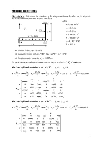
1. 1
MÉTODO DE RIGIDEZ
Ejercicio Nº 4: Determinar las reacciones y los diagramas finales de esfuerzos del siguiente
pórtico sometido a los estados de carga indicados.
Datos:
6 2
2
2
4
4
5
3 10 tn m
0.06 m
0.08 m
0.00045 m
0.00107 m
1.1 10 1 ºC
0.80 m
C
V
C
V
V
E
A
A
I
I
h
α −
= ⋅
=
=
=
=
= ⋅
=
a) Sistema de fuerzas exteriores.
b) Variación térmica en barra “AB”: 20ºST C∆ = y 0ºIT C∆ = .
c) Desplazamiento impuesto: 0.015 mA
yu = − .
En todos los casos considerar como variante un resorte en el nudo C: 2400 tn/mC
xk =
Matriz de rigidez elemental de la barra “AB” 1 21 ; 0γ γ= =
1 2 33 2
tn 12 tn 6 4
60000 ; 600 ; 1200 tn ; 3200 tn.m
m m
EA EI EI EI
K K K K
L L L L
⋅ ⋅ ⋅
= = = = = = = =
Matriz de rigidez elemental de la barra “BC” 1 20 ; 1γ γ= =
1 2 33 2
tn 12 tn 6 4
60000 ; 600 ; 900 tn ; 1800 tn.m
m m
EA EI EI EI
K K K K
L L L L
⋅ ⋅ ⋅
= = = = = = = =
4 m
A
B
q = 1.5 tn/m
C
P = 2 tn
3 m
x
y
A
60000 0 0 60000 0 0
0 600 1200 0 600 1200
0 1200 3200 0 1200 1600
60000 0 0 60000 0 0
0 600 1200 0 600 1200
0 1200 1600 0 1200 3200
ABK
−⎡ ⎤
⎢ ⎥−⎢ ⎥
⎢ ⎥−
= ⎢ ⎥
−⎢ ⎥
⎢ ⎥− − −
⎢ ⎥
−⎣ ⎦
B
A
B
B
600 0 900 600 0 900
0 60000 0 0 60000 0
900 0 1800 900 0 900
600 0 900 600 0 900
0 60000 0 0 60000 0
900 0 900 900 0 1800
BCK
− − −⎡ ⎤
⎢ ⎥−⎢ ⎥
⎢ ⎥−
= ⎢ ⎥
−⎢ ⎥
⎢ ⎥−
⎢ ⎥
−⎣ ⎦
B
C
C

2. 2
a) Sistema de fuerzas exteriores
Estado “I”
Estado “II”
60000 0 0 60000 0 0 0 0 0
0 600 1200 0 600 1200 0 0 0
0 1200 3200 0 1200 1600 0 0 0
60000 0 0 60600 0 900 600 0 900
0 600 1200 0 60600 1200 0 60000 0
0 1200 1600 900 1200 5000 900 0 900
0 0 0 600 0 900 600 0 900
0 0 0 0 60000 0 0 60000 0
0 0 0 900 0 900 900 0 1800
−
−
−
− − − −
− − − −
− −
−
−
−
0
3
2
1
3
1.25
1
0
0.75
A
x
A
y
A
z
B
x
B
y
B
z
C
x
C
y
C
z
u
u
u
u
u
u
φ
φ
φ
⎡ ⎤ ⎡ ⎤⎡ ⎤
⎢ ⎥ ⎢ ⎥⎢ ⎥ −⎢ ⎥ ⎢ ⎥⎢ ⎥
⎢ ⎥ ⎢ ⎥−⎢ ⎥
⎢ ⎥ ⎢ ⎥⎢ ⎥
⎢ ⎥ ⎢ ⎥⎢ ⎥
⎢ ⎥ ⎢ ⎥⎢ ⎥ = −
⎢ ⎥ ⎢ ⎥⎢ ⎥
⎢ ⎥ ⎢ ⎥⎢ ⎥
⎢ ⎥ ⎢ ⎥⎢ ⎥
⎢ ⎥ ⎢ ⎥⎢ ⎥
⎢ ⎥ ⎢ ⎥⎢ ⎥
⎢ ⎥ ⎢ ⎥⎢ ⎥
⎢ ⎥ ⎢ ⎥⎣ ⎦⎣ ⎦ ⎣ ⎦
B
2
2
0 0
2 3
12 2
0 0
2 3
12 2
AB
ABI
AB
AB
AB
qL
qL
P
qL
qL
⎡ ⎤ ⎡ ⎤
⎢ ⎥ ⎢ ⎥
⎢ ⎥ ⎢ ⎥
⎢ ⎥ ⎢ ⎥
= =⎢ ⎥ ⎢ ⎥
⎢ ⎥ ⎢ ⎥
⎢ ⎥ ⎢ ⎥
⎢ ⎥ ⎢ ⎥
− −⎢ ⎥ ⎣ ⎦⎣ ⎦
A
C
2 1
0 0
8 0.75
2 1
0 0
8 0.75
BCI
BC
BC
P
PL
P
P
PL
− −⎡ ⎤ ⎡ ⎤
⎢ ⎥ ⎢ ⎥
⎢ ⎥ ⎢ ⎥
⎢ ⎥ ⎢ ⎥
= =⎢ ⎥ ⎢ ⎥
− −⎢ ⎥ ⎢ ⎥
⎢ ⎥ ⎢ ⎥
⎢ ⎥ ⎢ ⎥
− −⎢ ⎥ ⎣ ⎦⎣ ⎦
B
A
1.5 tn/m
B
2.000 2.000
0.000 0.000
3.000 3.000
3.000 Q
A B
3.000
A B
nulo
N
2.000 Mf
A B
2.000
1.000
B
C
2
0.750
1.000
0.000
1.000
0.0000.750
B
C
N
nulo
B
C0.750
0.750
0.750
Mf
C
Q
1.000
1.000 B

3. 3
5
4
60600 900 1 2.027 10 m
900 5000 1.25 2.536 10 rad
B B
x x
B B
z z
u u
φ φ
−
−
− ⎡ ⎤ ⎧ = ⋅⎡ ⎤ ⎡ ⎤
= ⇒ ⎨⎢ ⎥⎢ ⎥ ⎢ ⎥− = ⋅⎣ ⎦ ⎣ ⎦⎣ ⎦ ⎩
5
4
0 1.216
0 0.304
0 0.406
2.027 10 1.216
0 0.304
2.536 10 0.812
AB
II
AB AB
U
P K −
−
−⎡ ⎤ ⎡ ⎤
⎢ ⎥ ⎢ ⎥
⎢ ⎥ ⎢ ⎥
⎢ ⎥ ⎢ ⎥
= ⋅ =⎢ ⎥ ⎢ ⎥
⋅⎢ ⎥ ⎢ ⎥
⎢ ⎥ ⎢ ⎥−
⎢ ⎥ ⎢ ⎥
⋅⎣ ⎦ ⎣ ⎦1442443
5
4
0.2162.027 10
00
0.4382.536 10
0.2160
00
0.2100
BC
II
BC BC
U
P K
−
−
−⎡ ⎤⋅ ⎡ ⎤
⎢ ⎥ ⎢ ⎥
⎢ ⎥ ⎢ ⎥
⎢ ⎥ ⎢ ⎥⋅
= ⋅ =⎢ ⎥ ⎢ ⎥
⎢ ⎥ ⎢ ⎥
⎢ ⎥ ⎢ ⎥
⎢ ⎥ ⎢ ⎥
⎢ ⎥ ⎣ ⎦⎣ ⎦1442443
Fuerzas totales de extremo de barras (Estado “I” + Estado “II”)
1.216
3.304
2.406
1.216
2.696
1.188
I II
AB AB ABP P P
−⎡ ⎤
⎢ ⎥
⎢ ⎥
⎢ ⎥
= + = ⎢ ⎥
⎢ ⎥
⎢ ⎥
⎢ ⎥
−⎣ ⎦
1.216
0
1.188
0.784
0
0.540
I II
BC BC BCP P P
−⎡ ⎤
⎢ ⎥
⎢ ⎥
⎢ ⎥
= + = ⎢ ⎥
−⎢ ⎥
⎢ ⎥
⎢ ⎥
−⎣ ⎦
A B
0.406 0.812
1.216 1.216
0.304 0.304
A B
1.216
N
+
0.406 Mf
A B
0.812
0.304
Q
A B
B
C
0.438
0.216
0.000
0.216
0.0000.210
B
C0.210
0.438
Mf
B
C
N
nulo
B
C
Q
0.216

4. 4
a') Sistema de fuerzas exteriores c/ resorte en nudo C: 2400 tn/mC
xk =
Estado “I”: Idem
Estado “II”
60000 0 0 60000 0 0 0 0 0
0 600 1200 0 600 1200 0 0 0
0 1200 3200 0 1200 1600 0 0 0
60000 0 0 60600 0 900 600 0 900
0 600 1200 0 60600 1200 0 60000 0
0 1200 1600 900 1200 5000 900 0 900
0 0 0 600 0 900 0 900
0 0 0 0 60000 0 0 60000 0
0 0 0 900 0 900 900 0 180
−
−
−
− − − −
− − − −
− −
−
−
−
3000
0
3
2
1
3
1.25
1
0
0 0.75
A
x
A
y
A
z
B
x
B
y
B
z
C
x
C
y
C
z
u
u
u
u
u
u
φ
φ
φ
⎡ ⎤ ⎡ ⎤⎡ ⎤
⎢ ⎥ ⎢ ⎥⎢ ⎥ −⎢ ⎥ ⎢ ⎥⎢ ⎥
⎢ ⎥ ⎢ ⎥−⎢ ⎥
⎢ ⎥ ⎢ ⎥⎢ ⎥
⎢ ⎥ ⎢ ⎥⎢ ⎥
⎢ ⎥ ⎢ ⎥⎢ ⎥ −=⎢ ⎥ ⎢ ⎥⎢ ⎥
⎢ ⎥ ⎢ ⎥⎢ ⎥
⎢ ⎥ ⎢ ⎥⎢ ⎥
⎢ ⎥ ⎢ ⎥⎢ ⎥
⎢ ⎥ ⎢ ⎥⎢ ⎥
⎢ ⎥ ⎢ ⎥⎢ ⎥
⎢ ⎥ ⎢ ⎥⎣ ⎦⎣ ⎦ ⎣ ⎦
5
4
4
60600 900 600 1 2.227 10 m
900 5000 900 1.25 2.042 10 rad
600 900 3000 1 2.765 10 m
B B
x x
B B
z z
C C
x x
u u
u u
φ φ
−
−
−
⎡ ⎤ ⎧− − = ⋅⎡ ⎤ ⎡ ⎤
⎢ ⎥ ⎪⎢ ⎥ ⎢ ⎥− = ⇒ = ⋅⎨⎢ ⎥⎢ ⎥ ⎢ ⎥
⎪⎢ ⎥⎢ ⎥ ⎢ ⎥− = ⋅⎣ ⎦ ⎣ ⎦⎣ ⎦ ⎩
A
1.5 tn/m
B
2.406 1.188
1.216 1.216
3.304 2.696
2.406 Mf
A B
1.188
1.203
3.304
Q
A B
2.696
A B
1.216
N
+
B
C
2
1.188
1.216
0.000
0.784
0.0000.540
B
C0.540
1.188
0.636
Mf
B
C
N
nulo
B
C
Q
0.784
1.216

5. 5
5
4
0 1.336
0 0.245
0 0.327
2.227 10 1.336
0 0.245
2.042 10 0.653
AB
II
AB AB
U
P K −
−
−⎡ ⎤ ⎡ ⎤
⎢ ⎥ ⎢ ⎥
⎢ ⎥ ⎢ ⎥
⎢ ⎥ ⎢ ⎥
= ⋅ =⎢ ⎥ ⎢ ⎥
⋅⎢ ⎥ ⎢ ⎥
⎢ ⎥ ⎢ ⎥−
⎢ ⎥ ⎢ ⎥
⋅⎣ ⎦ ⎣ ⎦1442443
5
4
4
0.3362.227 10
00
0.5962.042 10
0.3362.765 10
00
0.4130
BC
II
BC BC
U
P K
−
−
−
−⎡ ⎤⋅ ⎡ ⎤
⎢ ⎥ ⎢ ⎥
⎢ ⎥ ⎢ ⎥
⎢ ⎥ ⎢ ⎥⋅
= ⋅ =⎢ ⎥ ⎢ ⎥
⋅⎢ ⎥ ⎢ ⎥
⎢ ⎥ ⎢ ⎥
⎢ ⎥ ⎢ ⎥
⎢ ⎥ ⎣ ⎦⎣ ⎦1442443
Fuerzas totales de extremo de barras (Estado “I” + Estado “II”)
1.336
3.245
2.327
1.336
2.755
1.347
I II
AB AB ABP P P
−⎡ ⎤
⎢ ⎥
⎢ ⎥
⎢ ⎥
= + = ⎢ ⎥
⎢ ⎥
⎢ ⎥
⎢ ⎥
−⎣ ⎦
1.336
0
1.347
0.664
0
0.337
I II
BC BC BCP P P
−⎡ ⎤
⎢ ⎥
⎢ ⎥
⎢ ⎥
= + = ⎢ ⎥
−⎢ ⎥
⎢ ⎥
⎢ ⎥
−⎣ ⎦
Los diagramas se obtienen en forma análoga.
b) Variación térmica en barra “AB”
Estado “I” (sólo barra “AB”)
0
0
26.4 tn
2
0.88 tn.m
S I
S I
T T
N EA
T T
M EI
h
α
α
∆ + ∆⎛ ⎞
= =⎜ ⎟
⎝ ⎠
∆ − ∆⎛ ⎞
= =⎜ ⎟
⎝ ⎠
Estado “II”
4
4
60600 900 26.4 4.342 10 m
900 5000 0.88 9.785 10 rad
B B
x x
B B
z z
u u
φ φ
−
−
− ⎡ ⎤ ⎧ = ⋅⎡ ⎤ ⎡ ⎤
= ⇒ ⎨⎢ ⎥⎢ ⎥ ⎢ ⎥− − = − ⋅⎣ ⎦ ⎣ ⎦⎣ ⎦ ⎩
B
0
0
0
0
26.4
0 0
0.88
26.4
0 0
0.88
I
AB
N
M
P
N
M
⎡ ⎤ ⎡ ⎤
⎢ ⎥ ⎢ ⎥
⎢ ⎥ ⎢ ⎥
⎢ ⎥ ⎢ ⎥− −
= =⎢ ⎥ ⎢ ⎥
− −⎢ ⎥ ⎢ ⎥
⎢ ⎥ ⎢ ⎥
⎢ ⎥ ⎢ ⎥
⎢ ⎥ ⎣ ⎦⎣ ⎦
A
A B
0.880 0.880
26.4 26.4
0.000 0.000
A B
26.4
N
−
A B
nulo
Q 0.880
Mf
A B

6. 6
60000 0 0 60000 0 0 0 0 0
0 600 1200 0 600 1200 0 0 0
0 1200 3200 0 1200 1600 0 0 0
60000 0 0 60600 0 900 600 0 900
0 600 1200 0 60600 1200 0 60000 0
0 1200 1600 900 1200 5000 900 0 900
0 0 0 600 0 900 600 0 900
0 0 0 0 60000 0 0 60000 0
0 0 0 900 0 900 900 0 1800
−
−
−
− − − −
− − − −
− −
−
−
−
26.4
0
0.88
26.4
0
0.88
0
0
0
A
x
A
y
A
z
B
x
B
y
B
z
C
x
C
y
C
z
u
u
u
u
u
u
φ
φ
φ
−⎡ ⎤ ⎡ ⎤⎡ ⎤
⎢ ⎥ ⎢ ⎥⎢ ⎥
⎢ ⎥ ⎢ ⎥⎢ ⎥
⎢ ⎥ ⎢ ⎥⎢ ⎥
⎢ ⎥ ⎢ ⎥⎢ ⎥
⎢ ⎥ ⎢ ⎥⎢ ⎥
⎢ ⎥ ⎢ ⎥⎢ ⎥ =
⎢ ⎥ ⎢ ⎥⎢ ⎥
⎢ ⎥ ⎢ ⎥⎢ ⎥ −
⎢ ⎥ ⎢ ⎥⎢ ⎥
⎢ ⎥ ⎢ ⎥⎢ ⎥
⎢ ⎥ ⎢ ⎥⎢ ⎥
⎢ ⎥ ⎢ ⎥⎢ ⎥
⎢ ⎥ ⎢ ⎥⎣ ⎦⎣ ⎦ ⎣ ⎦
4
5
0 26.052
0 0.117
0 0.157
4.342 10 26.052
0 0.117
9.785 10 0.313
AB
II
AB AB
U
P K −
−
−⎡ ⎤ ⎡ ⎤
⎢ ⎥ ⎢ ⎥−⎢ ⎥ ⎢ ⎥
⎢ ⎥ ⎢ ⎥−
= ⋅ =⎢ ⎥ ⎢ ⎥
⋅⎢ ⎥ ⎢ ⎥
⎢ ⎥ ⎢ ⎥
⎢ ⎥ ⎢ ⎥
− ⋅ −⎣ ⎦ ⎣ ⎦1442443
4
5
0.3484.342 10
00
0.5679.785 10
0.3480
00
0.4790
BC
II
BC BC
U
P K
−
−
⎡ ⎤⋅ ⎡ ⎤
⎢ ⎥ ⎢ ⎥
⎢ ⎥ ⎢ ⎥
⎢ ⎥ ⎢ ⎥−− ⋅
= ⋅ =⎢ ⎥ ⎢ ⎥
−⎢ ⎥ ⎢ ⎥
⎢ ⎥ ⎢ ⎥
⎢ ⎥ ⎢ ⎥
−⎢ ⎥ ⎣ ⎦⎣ ⎦1442443
A B
0.157 0.313
26.05 26.05
0.117 0.117
A B
26.05
N
+
0.157
Mf
A B
0.313 0.117
Q
A B
B
C0.479
0.567
Mf
B
C
N
nulo
B
C
Q
0.348
C
0.567
0.348
0.000
0.348
0.0000.479
B

7. 7
Fuerzas totales de extremo de barras (Estado “I” + Estado “II”)
0.348
0.117
1.037
0.348
0.117
0.567
I II
AB AB ABP P P
⎡ ⎤
⎢ ⎥−⎢ ⎥
⎢ ⎥−
= + = ⎢ ⎥
−⎢ ⎥
⎢ ⎥
⎢ ⎥
⎣ ⎦
0.348
0
0.567
0.348
0
0.479
I II
BC BC BCP P P
⎡ ⎤
⎢ ⎥
⎢ ⎥
⎢ ⎥−
= + = ⎢ ⎥
−⎢ ⎥
⎢ ⎥
⎢ ⎥
−⎣ ⎦
Los diagramas finales de la barra “BC” coinciden con los del Estado “II”.
b') Variación térmica en barra “AB” c/ resorte en nudo C: 2400 tn/mC
xk =
Estado “I”: Idem
Estado “II”
60000 0 0 60000 0 0 0 0 0
0 600 1200 0 600 1200 0 0 0
0 1200 3200 0 1200 1600 0 0 0
60000 0 0 60600 0 900 600 0 900
0 600 1200 0 60600 1200 0 60000 0
0 1200 1600 900 1200 5000 900 0 900
0 0 0 600 0 900 0 900
0 0 0 0 60000 0 0 60000 0
0 0 0 900 0 900 900 0 180
−
−
−
− − − −
− − − −
− −
−
−
−
3000
26.4
0
0.88
26.4
0
0.88
0
0
0 0
A
x
A
y
A
z
B
x
B
y
B
z
C
x
C
y
C
z
u
u
u
u
u
u
φ
φ
φ
−⎡ ⎤ ⎡ ⎤⎡ ⎤
⎢ ⎥ ⎢ ⎥⎢ ⎥
⎢ ⎥ ⎢ ⎥⎢ ⎥
⎢ ⎥ ⎢ ⎥⎢ ⎥
⎢ ⎥ ⎢ ⎥⎢ ⎥
⎢ ⎥ ⎢ ⎥⎢ ⎥
⎢ ⎥ ⎢ ⎥⎢ ⎥ =⎢ ⎥ ⎢ ⎥⎢ ⎥
⎢ ⎥ ⎢ ⎥−⎢ ⎥
⎢ ⎥ ⎢ ⎥⎢ ⎥
⎢ ⎥ ⎢ ⎥⎢ ⎥
⎢ ⎥ ⎢ ⎥⎢ ⎥
⎢ ⎥ ⎢ ⎥⎢ ⎥
⎢ ⎥ ⎢ ⎥⎣ ⎦⎣ ⎦ ⎣ ⎦
4
4
4
60600 900 600 26.4 4.351 10 m
900 5000 900 0.88 1.198 10 rad
600 900 3000 0 1.230 10 m
B B
x x
B B
z z
C C
x x
u u
u u
φ φ
−
−
−
⎡ ⎤ ⎧− − = ⋅⎡ ⎤ ⎡ ⎤
⎢ ⎥ ⎪⎢ ⎥ ⎢ ⎥− = − ⇒ = − ⋅⎨⎢ ⎥⎢ ⎥ ⎢ ⎥
⎪⎢ ⎥⎢ ⎥ ⎢ ⎥− = ⋅⎣ ⎦ ⎣ ⎦⎣ ⎦ ⎩
A B
1.037 0.567
0.348 0.348
0.117 0.117
A B
0.348
N
–
1.037
Mf
A B
0.567
0.117
Q

8. 8
4
4
0 26.106
0 0.144
0 0.192
4.351 10 26.106
0 0.144
1.198 10 0.383
AB
II
AB AB
U
P K −
−
−⎡ ⎤ ⎡ ⎤
⎢ ⎥ ⎢ ⎥−⎢ ⎥ ⎢ ⎥
⎢ ⎥ ⎢ ⎥−
= ⋅ =⎢ ⎥ ⎢ ⎥
⋅⎢ ⎥ ⎢ ⎥
⎢ ⎥ ⎢ ⎥
⎢ ⎥ ⎢ ⎥
− ⋅ −⎣ ⎦ ⎣ ⎦1442443
4
4
4
0.2954.351 10
00
0.4971.198 10
0.2951.230 10
00
0.3890
BC
II
BC BC
U
P K
−
−
−
⎡ ⎤⋅ ⎡ ⎤
⎢ ⎥ ⎢ ⎥
⎢ ⎥ ⎢ ⎥
⎢ ⎥ ⎢ ⎥−− ⋅
= ⋅ =⎢ ⎥ ⎢ ⎥
−⋅⎢ ⎥ ⎢ ⎥
⎢ ⎥ ⎢ ⎥
⎢ ⎥ ⎢ ⎥
−⎢ ⎥ ⎣ ⎦⎣ ⎦1442443
Fuerzas totales de extremo de barras (Estado “I” + Estado “II”)
0.295
0.144
1.072
0.295
0.144
0.497
I II
AB AB ABP P P
⎡ ⎤
⎢ ⎥−⎢ ⎥
⎢ ⎥−
= + = ⎢ ⎥
−⎢ ⎥
⎢ ⎥
⎢ ⎥
⎣ ⎦
0.295
0
0.497
0.295
0
0.389
I II
BC BC BCP P P
⎡ ⎤
⎢ ⎥
⎢ ⎥
⎢ ⎥−
= + = ⎢ ⎥
−⎢ ⎥
⎢ ⎥
⎢ ⎥
−⎣ ⎦
Los diagramas se obtienen en forma análoga.
c) Desplazamiento impuesto: 0.015 mA
yu = −
Estado Final: únicamente participa el Estado “II”.
60000 0 60000 0 0 0 0 0
0 1200 0 600 1200 0 0 0
0 3200 0 1200 1600 0 0 0
60000 0 60600 0 900 600 0 900
0 1200 0 60600 1200 0 60000 0
0 1600 900 1200 5000 900 0 900
0 0 600 0 900 600 0 900
0 0 0 60000 0 0 60000 0
0 0 900 0 900 900 0 1800
−⎡ ⎤
⎢ ⎥−⎢ ⎥
⎢ ⎥−
⎢
− − − −⎢
⎢ − − −
⎢
⎢ − −
⎢
−⎢
⎢ −
⎢
−⎢⎣ ⎦
0 0
600 9
1200 18
0 0
600 9
1200 18
0 0
0 0
0 0
A
x
A
z
B
x
B
Ay
yB
z
C
x
C
y
C
z
u
u
u
u
u
u
φ
φ
φ
⎡ ⎤ ⎡ ⎤
⎡ ⎤ ⎢ ⎥ ⎢ ⎥
⎢ ⎥ ⎢ ⎥ ⎢ ⎥
⎢ ⎥ ⎢ ⎥ ⎢ ⎥
⎢ ⎥⎥ ⎢ ⎥ ⎢ ⎥
⎢ ⎥⎥ ⎢ ⎥ ⎢ ⎥
⎢ ⎥⎥ ⎢ ⎥ ⎢ ⎥= − =− −
⎢ ⎥⎥ ⎢ ⎥ ⎢ ⎥
⎢ ⎥⎥ ⎢ ⎥ ⎢ ⎥
⎢ ⎥⎥ ⎢ ⎥ ⎢ ⎥
⎢ ⎥⎥ ⎢ ⎥ ⎢ ⎥
⎢ ⎥⎥ ⎢ ⎥ ⎢ ⎥
⎢ ⎥⎥ ⎢ ⎥ ⎢ ⎥⎣ ⎦
⎥ ⎢ ⎥ ⎢ ⎥⎣ ⎦ ⎣ ⎦
5
3
60600 900 0 5.361 10 m
900 5000 18 3.610 10 rad
B B
x x
B B
z z
u u
φ φ
−
−
− ⎡ ⎤ ⎧ = ⋅⎡ ⎤ ⎡ ⎤
= ⇒ ⎨⎢ ⎥⎢ ⎥ ⎢ ⎥− = ⋅⎣ ⎦ ⎣ ⎦⎣ ⎦ ⎩
5
3
0 3.217
0.015 4.668
0 12.22
5.361 10 3.217
0 4.668
3.610 10 6.449
AB
AB AB
U
P K −
−
−⎡ ⎤ ⎡ ⎤
⎢ ⎥ ⎢ ⎥− −⎢ ⎥ ⎢ ⎥
⎢ ⎥ ⎢ ⎥−
= ⋅ =⎢ ⎥ ⎢ ⎥
⋅⎢ ⎥ ⎢ ⎥
⎢ ⎥ ⎢ ⎥
⎢ ⎥ ⎢ ⎥
⋅ −⎣ ⎦ ⎣ ⎦1442443
5
3
3.2175.361 10
00
6.4493.610 10
3.2170
00
3.2010
BC
II
BC BC
U
P K
−
−
−⎡ ⎤⋅ ⎡ ⎤
⎢ ⎥ ⎢ ⎥
⎢ ⎥ ⎢ ⎥
⎢ ⎥ ⎢ ⎥⋅
= ⋅ =⎢ ⎥ ⎢ ⎥
⎢ ⎥ ⎢ ⎥
⎢ ⎥ ⎢ ⎥
⎢ ⎥ ⎢ ⎥
⎢ ⎥ ⎣ ⎦⎣ ⎦1442443

9. 9
c') Desplazamiento impuesto c/ resorte en nudo C: 2400 tn/mC
xk =
Estado Final: únicamente participa el Estado “II”.
60000 0 60000 0 0 0 0 0
0 1200 0 600 1200 0 0 0
0 3200 0 1200 1600 0 0 0
60000 0 60600 0 900 600 0 900
0 1200 0 60600 1200 0 60000 0
0 1600 900 1200 5000 900 0 900
0 0 600 0 900 0 900
0 0 0 60000 0 0 60000 0
0 0 900 0 900 900 0 1800
−⎡ ⎤
⎢ ⎥−⎢ ⎥
⎢ −
⎢
− − − −⎢
⎢ − − −
⎢
⎢ − −
⎢
−⎢
⎢
−⎢
⎢ −⎣ ⎦
3000
0 0
600 9
1200 18
0 0
600 9
1200 18
0 0
0 0
0 0
A
x
A
z
B
x
B
Ay
yB
z
C
x
C
y
C
z
u
u
u
u
u
u
φ
φ
φ
⎡ ⎤ ⎡ ⎤
⎢ ⎥ ⎢ ⎥⎡ ⎤
⎢ ⎥ ⎢ ⎥⎢ ⎥
⎥ ⎢ ⎥ ⎢ ⎥⎢ ⎥
⎥ ⎢ ⎥ ⎢ ⎥⎢ ⎥
⎥ ⎢ ⎥ ⎢ ⎥⎢ ⎥
⎥ ⎢ ⎥ ⎢ ⎥⎢ ⎥ − −= − =⎥ ⎢ ⎥ ⎢ ⎥⎢ ⎥
⎥ ⎢ ⎥ ⎢ ⎥⎢ ⎥
⎥ ⎢ ⎥ ⎢ ⎥⎢ ⎥
⎥ ⎢ ⎥ ⎢ ⎥⎢ ⎥
⎥ ⎢ ⎥ ⎢ ⎥⎢ ⎥
⎥ ⎢ ⎥ ⎢ ⎥⎢ ⎥⎣ ⎦
⎥ ⎢ ⎥ ⎢ ⎥⎣ ⎦ ⎣ ⎦
5
3
3
60600 900 600 0 4.539 10 m
900 5000 900 18 3.812 10 rad
600 900 3000 0 1.135 10 m
B B
x x
B B
z z
C C
x x
u u
u u
φ φ
−
−
−
⎡ ⎤ ⎧− − = ⋅⎡ ⎤ ⎡ ⎤
⎢ ⎥ ⎪⎢ ⎥ ⎢ ⎥− = ⇒ = ⋅⎨⎢ ⎥⎢ ⎥ ⎢ ⎥
⎪⎢ ⎥⎢ ⎥ ⎢ ⎥− = − ⋅⎣ ⎦ ⎣ ⎦⎣ ⎦ ⎩
A B
12.22 6.449
3.217 3.217
4.668 4.668
A B
3.217
N
+
12.22
Mf
A B
6.449
4.668
Q
A B
B
C
6.449
3.217
0.000
3.217
0.0003.201
B
C3.201
6.449
Mf
B
C
N
nulo
B
C
Q
3.217

10. 10
5
3
0 2.723
0.015 4.426
0 11.90
4.539 10 2.723
0 4.426
3.812 10 5.800
AB
AB AB
U
P K −
−
−⎡ ⎤ ⎡ ⎤
⎢ ⎥ ⎢ ⎥− −⎢ ⎥ ⎢ ⎥
⎢ ⎥ ⎢ ⎥−
= ⋅ =⎢ ⎥ ⎢ ⎥
⋅⎢ ⎥ ⎢ ⎥
⎢ ⎥ ⎢ ⎥
⎢ ⎥ ⎢ ⎥
⋅ −⎣ ⎦ ⎣ ⎦1442443
5
3
3
2.7234.539 10
00
5.8003.812 10
2.7231.135 10
00
2.3680
BC
BC BC
U
P K
−
−
−
−⎡ ⎤⋅ ⎡ ⎤
⎢ ⎥ ⎢ ⎥
⎢ ⎥ ⎢ ⎥
⎢ ⎥ ⎢ ⎥⋅
= ⋅ =⎢ ⎥ ⎢ ⎥
− ⋅⎢ ⎥ ⎢ ⎥
⎢ ⎥ ⎢ ⎥
⎢ ⎥ ⎢ ⎥
⎢ ⎥ ⎣ ⎦⎣ ⎦1442443
Los diagramas se obtienen en forma análoga.