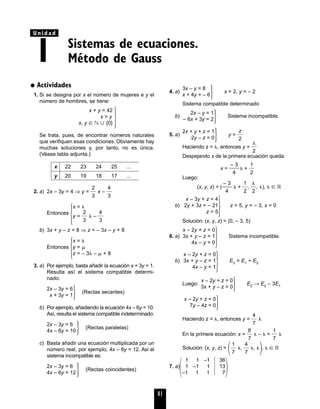
El documento presenta una serie de ejercicios relacionados con sistemas de ecuaciones. Incluye problemas para determinar si los sistemas son compatibles o incompatibles, determinados o indeterminados. También presenta ejemplos resueltos de sistemas compatibles determinados e indeterminados.


![C · D =
·
=
2. A = (1 –1 1), At
=
B =
, Bt
=
A · B t = (1 –1 1) ·
= (0 0)
B · At =
·
= (0, 0)
3. (A + B) (A – B) = A · A – A · B + B · A – B · B =
= A2
– AB + BA – B 2
= A2
– B 2
⇔
⇔ – AB + BA = 0 ⇔ AB = BA
Esto es: se verifica que (A + B) (A – B) = A2
– B 2
si, y sólo si, se emplea la propiedad conmutativa
del producto de matrices.
Ejemplo:
A =
, B =
A · B =
·
=
B · A =
·
=
AB BA, y, en consecuencia,
(A + B) · (A – B) A2
– B 2
4. Para que se puedan efectuar los productos A · B
y B · A, la matriz B debe tener dimensión 2 × 2.
Sea B =
la matriz buscada. Entonces:
A · B =
·
=
B · A =
·
=
·
AsÍ:
B =
5. A =
, B =
a) (A + B)2
=
·
=
b) A2
+ 2AB + B2
=
·
+
+ 2
·
+
·
=
=
c) (A + B)2
A2
+ 2AB + B2
porque A · B B · A.
6. Si A es una matriz cualquiera de orden m × n
entonces At
tendrá orden n × m. De tal forma que,
At
n × m
· Am × n
= At
· An × n
y
Am × n
· At
n × m
= A · At
m × m
Luego siempre existen los productos A · At
y At
· A.
7. P =
P2
=
·
=
Luego:
·
(1 – a)2 – (1 – a) = 0 →
→ (1 – a) [1 – a – 1] = 0 → Ά
En consecuencia:
c ʦ ޒ y a = 0 o a = 1
Existen matrices P tales que:
P =
o P =
1 0
c 0
0 0
c 1
a = 0
a = 1
→ a2 – a = 0 →
a = 0
→ a(a – 1) = 0 →
Άa = 1
a2
= a
(1 – a)2
= 1 – a
a2
0
c (1 – a)2
a 0
c 1 – a
a 0
c 1 – a
a 0
c 1 – a
–3 –6
–2 7
–2 0
1 2
–2 0
1 2
–2 0
1 2
1 –1
2 1
1 –1
2 1
1 –1
2 1
–2 –2
6 6
–1 –1
3 3
–1 –1
3 3
–2 0
1 2
1 –1
2 1
d – 2b b
0 d
c = 0
a = d – 2b
b, d ʦ ޒ
c = 0
d = a + 2b
2c = 0
2d = c + 2d
0 a + 2b
0 c + 2d
0 1
0 2
a b
c d
c d
2c 2d
a b
c d
0 1
0 2
a b
c d
0 –2 0
0 0 1
4 2 1
2 1 0
0 0 1
0 2 0
0 0 –1
0 1 0
2 1 0
0 1 –2
2 1 0
0 2 0
0 0 –1
0 1 0
2 1 0
2 1 0
0 0 1
0 2 0
0 0 –1
0 1 0
2 1 0
2 1 0
0 0 1
0 2 0
1
–1
1
2 3 1
4 8 4
2 4
3 8
1 4
2 4
3 8
1 4
2 3 1
4 8 4
1
–1
1
4 7
8 11
2 –1
0 3
2 3
4 5
59
01_unidades 1 a 3 25/5/04 12:17 Página 59](https://image.slidesharecdn.com/mcgrawhill-sol-bac-2-ccnn-2003-170728180142/85/Mc-grawhill-sol-bac-2-ccnn-2003-19-320.jpg)


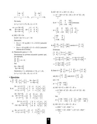
![a b c d e
M4
=
Por ejemplo, entre a y c hay 9 caminos de longi-
tud 4; mientras no hay ningún camino con esa
longitud entre a y d; siendo 5 el número de cami-
nos entre a y e.
Entre a y e los caminos son:
a - b - c - d - e; a - d - e -d - e; a - d - c - d - e;
a - b - a - d - e; a - d - a - d - e
10. La matriz de un giro de 30° es:
=
Entonces:
A′: (1 1) ·
=
=
B′: (2 3) ·
=
=
C′: (1 4) ·
=
=
Así:
A′
,
B′
,
C′
,
11. A2 =
, A =
c1 = a11 + a12 + a13 + a14 + ᎏ
1
2
ᎏ [a2
11 + a2
12 + a2
13 + a2
14] =
= 2 + ᎏ
3
2
ᎏ = ᎏ
5
2
ᎏ = 2,5
c2
= 1 + 1 = 2
c3
= 2 + 1 = 3
c4
= 1 + ᎏ
1
2
ᎏ = 1,5
Por tanto, la clasificación es la siguiente:
1.er clasificado, c3
, con 3 puntos
2.o
clasificado, c1, con 2,5 puntos
3.er
clasificado, c2
, con 2 puntos
4.º clasificado, c4
, con 1,5 puntos
• Márgenes
— Página 48.
Una matriz triangular y simétrica es, por ejemplo,
Salvo la matriz nula, no existe ninguna matriz
triangular y antisimétrica.
— Página 52.
(A · B)t = At · Bt (Falsa)
(A · B)t = Bt · At (Cierta)
— Página 54.
Por ejemplo, A =
y B =
A–1 =
y B –1 =
A–1 + B–1 =
y (A + B)–1 =
Luego, (A + B)–1
A–1
+ B–1
— Página 58.
Sí, es cierto. Basta aplicar la propiedad asociati-
va del producto de matrices.
A2 · A = (A · A) · A = A · (A · A) = A · A2
1/2 –1/4
0 1/2
2 –1
0 2
1 –1
0 1
1 0
0 1
1 1
0 1
1 0
0 1
1 0
0 3
0 0 1 1
1 0 0 0
0 1 0 1
0 1 0 0
0 2 0 1
0 0 1 1
1 1 0 0
1 0 0 0
–1 +4͙3ෆ
ᎏᎏ
2
͙3ෆ + 4
ᎏ
2
–2 + 3͙3ෆ
ᎏᎏ
2
2͙3ෆ + 3
ᎏᎏ
2
–1+ ͙3ෆ
ᎏ
2
͙3ෆ + 1
ᎏ
2
–1 +4͙3ෆ
ᎏᎏ
2
͙3ෆ + 4
ᎏ
2
͙3ෆ/2 –1/2
1/2 ͙3ෆ/2
–2 + 3͙3ෆ
ᎏᎏ
2
2͙3ෆ + 3
ᎏᎏ
2
͙3ෆ/2 –1/2
1/2 ͙3ෆ/2
–1+ ͙3ෆ
ᎏ
2
͙3ෆ + 1
ᎏ
2
͙3ෆ/2 –1/2
1/2 ͙3ෆ/2
͙3ෆ/2 –1/2
1/2 ͙3ෆ/2
cos 30° –sen 30°
sen 30° cos 30°
9 0 9 0 5
0 8 0 8 0
9 0 9 0 5
0 8 0 13 0
5 0 5 0 3
a
b
c
d
e
65
01_unidades 1 a 3 25/5/04 12:17 Página 65](https://image.slidesharecdn.com/mcgrawhill-sol-bac-2-ccnn-2003-170728180142/85/Mc-grawhill-sol-bac-2-ccnn-2003-25-320.jpg)


![15.
Έ Έ=
Έ Έ= 0, porque
c′3 = c3 – pc2
c1
= c′3
16. a)
Έ Έ= –1 ·
Έ Έ=
Desarrollando por la 2.a
fila
= –[12 – 24 – 36 – 8] = 56
b)
Έ Έ=
Έ Έ=
c′3
= c3
– 2c2
Desarrollando
por la 2.a fila
=
Έ Έ= –32 + 50 + 160 + 28 = 206
17.
Έ Έ= 0 ⇒
Έ Έ=
F′2
= F2
– F1
F′3
= F3
– F1
F′4
= F4
– F1
= x
Έ Έ=
Desarrollando por la 1.a columna
= x (–1(1 – x )3 + x3) = x (2x3 – 3x 2 + 3x – 1) = 0
⇒ x1 = 0, x2 = ᎏ
1
2
ᎏ, x3 = , x4 =
18. Si |M| = –5 ⇒ |M–1| = ᎏ
|M
1
|
ᎏ = ᎏ
1
5
ᎏ
19. • B =
|B| = 5 0 ⇒ ∃B–1
B–1 =
• C =
, |C| = 0 ⇒ ∃/ C–1
20. • |A| =
Έ Έ= 4 – 36 – 16 – 24 =
= –72 0 ⇒ rg (A) = 3
• |5| 0, Έ Έ= –10 0 ⇒ rg (B) = 2
• |–1| 0, Έ Έ= –3 0
Έ Έ= 0 y
Έ Έ= 0
Luego rg (C) = 2
• |–2| 0, Έ Έ= –7 0
Έ Έ= –21 0 ⇒ rg (D) = 3
21. A =
, a ʦ ޒ
a) rg (A) = 2 ⇔ |A| = 0
|A| = a2 – 1 = 0 ⇔ a = ±1
Por tanto, rg (A) = 2 si, y sólo si, a = ±1.
b) ∃A –1 ⇔ |A| 0 ⇔ a –1 y a 1.
De esta manera, rg (A) = 3.
• Ejercicios
1.
Έ Έ= –
Έ Έ=
Έ Έ=
F′1
= (–1)F1
F′2
= (–1)F2
= –
Έ Έ= –10
F′3
= (–1)F3
–a –b –c
–d –e –f
–g –h –i
–a –b –c
–d –e –f
g h i
–a –b –c
d e f
g h i
a b c
d e f
g h i
1 a 1
a –a 1
a 1 1
–2 1 0
3 2 0
0 0 3
–2 1
3 2
–1 4 3
0 3 1
2 –8 –6
–1 4 –5
0 3 6
2 –8 10
–1 4
0 3
0 2
5 0
1 0 2
3 –2 4
–4 6 –2
0 2 –3
1 0 5
1 2 2
–1 –3/5
0 1/5
1 3
0 5
1 + ͙3ෆi
ᎏ
2
1 – ͙3ෆi
ᎏ
2
1 – x –x 0
–x 0 1 – x
0 1 – x –x
x x x x
0 1 – x –x 0
0 –x 0 1 – x
0 0 1 – x –x
x x x x
x 1 0 x
x 0 x 1
x x 1 0
2 5 4
0 –8 2
5 7 2
2 –1 5 4
0 1 0 0
0 3 –8 2
5 0 7 2
2 –1 3 4
0 1 2 0
0 3 –2 2
5 0 7 2
1 –2 2
–2 6 4
3 0 2
1 –2 5 2
0 0 1 0
–2 6 7 4
3 0 1 2
a d a
b e b
c f c
a d a + pd
b e b + pe
c f c + pf
68
01_unidades 1 a 3 25/5/04 12:17 Página 68](https://image.slidesharecdn.com/mcgrawhill-sol-bac-2-ccnn-2003-170728180142/85/Mc-grawhill-sol-bac-2-ccnn-2003-28-320.jpg)


![At · X =
·
=
A · Xt =
·
=
Si At
· X = A · X t
⇒
Ά ⇒
⇒
Ά → –x – y = a(x + y) ⇒
⇒ a = –1 → 2y – x = 2z – x → y = z
Luego:
X =
, si x –y y a = –1
X =
, si a –1
8. |A| = 2 y |B | = 3
|B–1
· A · B| = |B –1
| · |A| · |B | = |A| = 2
ll
1
9.
Έ Έ=
Έ Έ=
F′2 = F2 – 2F1 Desarrollando por
F′3 = F3 + F1 la 1.a
columna
=
Έ Έ= 0
Por ejemplo: Έ Έ= –2 0
y
Έ Έ= –2 0
Por tanto: rg (A ) = 3.
10. 2A2
= A ⇒ |2A 2
| = |A | ⇒ 22
· |A2
| = |A| ⇒
⇒ 4|A| · |A| = |A| ⇒ 4|A | · |A| – |A| = 0 ⇒
⇒ |A| (4|A| –1) = 0 ⇒ |A | = 0 o |A| = 1/4
11. A =
, B =
A · B =
·
=
|A · B| = (2x + 1) – (–x + 1)(2x + 3) = 2x2
+ 3x – 2
Entonces ∃(A · B)–1
⇔ |A · B| 0
2x2 + 3x – 2 0 ⇔ x –2 y x 12.
12. |A| =
Έ Έ=
F′1 = F1 – F4
F′2 = F2 – F4
F′3 = F3 – F4
=
Έ Έ=
F″1 = F′1 – aF′4
=
Έ Έ=
Desarrollando por la 1.a
columna
= –
Έ Έ=
= –[(b – a + ab) (–ab) + ab2 – a2b] = a2b2
Por otro lado,
Έ Έ= –a2
, Έ Έ= 0
Έ Έ= –b2
Luego:
|B| = Έ Έ= a2
b2
En efecto, pues |A| = |B |
13. M =
|M| = 2 0, ∀ a, b ʦ ޒ
1 a 0
a a2
+ 2 2b
0 2b 2b2
+ 1
–a2
0
0 –b2
1 + b 1
1 1 – b
1 1
1 1
1 + a 1
1 1 – a
–a –a b – a + ab
–a 0 b
0 b b
0 –a –a b – a + ab
0 –a 0 b
0 0 b b
1 1 1 1 – b
a 0 0 b
0 –a 0 b
0 0 b b
1 1 1 1 – b
1 + a 1 1 1
1 1 – a 1 1
1 1 1 + b 1
1 1 1 1 – b
2x + 1 2x + 3
–x + 1 1
1 3
x 0
0 2
1 2 x
1 –1 –1
1 3
x 0
0 2
1 2 x
1 –1 –1
1 0 –1
2 –2 1
–1 –1 3
1 0
2 –2
–2 3 5
–1 2 3
–1 1 2
1 0 –1 1
0 –2 3 5
0 –1 2 3
0 –1 1 2
1 0 –1 1
2 –2 1 7
–1 –1 3 2
0 –1 1 2
x –x
–x x
x y
y x
az = –y
2y + ax = 2z – x
–x + az = ax + ay
2x + az = 2x – y
2y + ax = 2z – x
–x + az = ax + ay
–y + ax = az + ax
2x – y 2z – x
ax + ay az + ax
x z
y x
2 –1
a a
2x + az 2y + ax
–x + az –y + ax
x y
z x
2 a
–1 a
74
01_unidades 1 a 3 25/5/04 12:17 Página 74](https://image.slidesharecdn.com/mcgrawhill-sol-bac-2-ccnn-2003-170728180142/85/Mc-grawhill-sol-bac-2-ccnn-2003-34-320.jpg)


![2. x = número de hombres.
y = número de mujeres.
z = número de niños.
·⇒
·
Έ Έx = ᎏᎏᎏᎏᎏᎏᎏ = ᎏ
5
8
6
ᎏ = 7
8
Έ Έy = ᎏᎏᎏᎏᎏᎏᎏᎏ = ᎏ
18
8
4
ᎏ = 23
8
De la primera ecuación: z = 40 – 7 – 23 = 10
En consecuencia, en la reunión habría 7 hom-
bres, 23 mujeres y 10 niños.
3. x = calificación obtenida en el 1.er
examen parcial.
y = calificación obtenida en el 2.o
examen parcial.
z = calificación obtenida en el examen final.
= 6
0,20x + 0,20y + 0,60z = 7,6
0,10x + 0,20y + 0,70z = 8,3
⇒
· Έ Έ= –2
Έ Έx = ᎏᎏᎏᎏᎏᎏ = ᎏ
–
–
6
2
ᎏ = 3
–2
Έ Έy = ᎏᎏᎏᎏᎏᎏᎏ = ᎏ
–
–
1
2
0
ᎏ = 5
–2
De la primera ecuación: z = 10
En consecuencia, Luis obtuvo en la primera eva-
luación las siguientes calificaciones: 3, 5 y 10.
4. Sean:
x = edad actual de la madre.
y = edad actual del hijo mayor.
z = edad actual del hijo menor.
Entonces hace 14 años las edades de la madre y
de los dos hijos eran, respectivamente, x – 14,
y – 14, z – 14. Luego:
x – 14 = 5[(y – 14) + (z – 14)]
Dentro de 10 años las edades respectivas serán:
x + 10, y + 10, z + 10. Por tanto:
x + 10 = (y + 10) + (z + 10)
Por otra parte, dentro de m años se cumplirá:
y + m = x
z + m = 42
Por consiguente, el sistema a que da lugar el
enunciado es:
·
La edad de la madre es de 44 años, siendo 18 y
16 las edades de los hijos.
5.
·⇒
·
Haciendo z =
Έ Έ
x = ᎏᎏᎏᎏᎏᎏᎏᎏᎏ = ᎏ
1 +
4
5
ᎏ
4
Έ Έ
y = ᎏᎏᎏᎏᎏᎏᎏᎏ = ᎏ
44 – 10
4
– 9 +
ᎏ =
4
= ᎏ
35 –
4
9
ᎏ
(x, y, z) =
ᎏ
1 +
4
5
ᎏ, ᎏ
35 –
4
9
ᎏ,
Como x у 0, y у 0, z у 0 y, además, x, y, z ʦ ޚ
entonces:
x = ᎏ
1 +
4
5
ᎏ у 0, y = ᎏ
35 –
4
9
ᎏ у 0, z = у 0,
ʦ ޚ
1 + 5 у 0, 35 – 9 у 0, у 0, ʦ ޚ
у –ᎏ
1
5
ᎏ, р ᎏ
3
9
5
ᎏ, у 0, ʦ ޚ
•––––•––––•––––•––––•
0 1 2 3 35/9
1 9 –
1 44 – 10
9 – 1
44 – 10 5
x + y = 9 –
x + 5y = 44 – 10
x + y + z = 9
x + 5y + 10z = 44
x = 44
y = 18
z = 16
m = 26
x – 5y – 5z = –126
x – y – z = 10
–x + y + m = 0
z + m = 42
1 18 1
1 38 3
1 83 7
18 1 1
38 1 3
83 2 7
1 1 1
1 1 3
1 2 7
x + y + z = 18
x + y + 3z = 38
x + 2y + 7z = 83
x + y + z
ᎏᎏ
3
1 40 1
1 0 –3
–1 6 –1
40 1 1
0 1 –3
6 1 –1
x + y + z = 40
x + y – 3z = 0
–x + y – z = 6
x + y + z = 40
x + y = 3z
y = x + z + 6
90
·⇒
02_unidades 4 a 5 25/5/04 12:19 Página 90](https://image.slidesharecdn.com/mcgrawhill-sol-bac-2-ccnn-2003-170728180142/85/Mc-grawhill-sol-bac-2-ccnn-2003-50-320.jpg)


![29. u × v =
Έ Έ= 19i – 16j – 23k
30. w = u × v =
Έ Έ= –5i – 5j – 5k
w
1 = ᎏ
|
w
w
|
ᎏ = =
= – i – j – k
w
5
= 5 · w
1
= – i – j – k
o
w′
5
= i + j+ k.
31. w = au + bv
(u + v + w) × (u – v – w) =
= [(1 + a)u + (1 + b)v] × [(1 – a)u – (1 + b)v] =
= – (1 + a)(1 + b)u × v – (1 – a)(1 + b)u × v =
= –[(1 + a)(1 + b) + (1 – a)(1 + b)]u × v =
= –[(1 + a + 1 – a)(1 + b)]u × v = –2(1 + b)u × v
32. [u, v, w] =
Έ Έ= –19
33. APar.
= |u × v| =
͙Έ Έ
2
+
Έ Έ
2
+
Έ Έ
2
=
= ͙1 + 1ෆ+ 0ෆ = ͙2ෆ u2
34. ATriang. = ᎏ
1
2
ᎏ APar. = ᎏ
1
2
ᎏ |AB × AC| =
= ᎏ
1
2
ᎏ ͙9 + 0ෆ+ 81ෆ = ᎏ
1
2
ᎏ ͙90ෆ = ᎏ
3
2
ᎏ ͙10ෆ
·= AB × AC =
=
Έ Έ= 3i + 0j – 9k
35. AParalelep.
= [u, v, w]| =
ΈΈ ΈΈ= 13 u3
36. VTetraedro
= ᎏ
1
6
ᎏ |[AB, AC, AD]| = ᎏ
1
6
ᎏ
ΈΈ ΈΈ=
= ᎏ
1
6
ᎏ · 5 = ᎏ
5
6
ᎏ u3
37. AB · AC = 0 ⇒ (3, 4, 4) · (2, 3, – 1) = 0
6 + 12 + 4( – 1) = 0; – 1 = –ᎏ
1
4
8
ᎏ = –ᎏ
9
2
ᎏ
= –ᎏ
7
2
ᎏ
A = ᎏ
1
2
ᎏ ͙9 + 16ෆ + 16ෆ · Ί4 + 9+=
= Ӎ 18,46
AB × AC =
Έ Έ= –30i + ᎏ
4
2
3
ᎏ j + k
A = ᎏ
1
2
ᎏ |AB × AC| = = Ӎ 18,46
38. AB = CD ⇒ AC = BD, BA = DC, CA = DB
1) AD = AD ⇒ AB + BD = AC + CD ⇒
⇒ AB + BD = AC + AB ⇒ BD = AC
2) Como ΈAB = CD ⇒
⇒ – AB = – CD ⇒ BA = DC
3) A partir de 1) y 2) queda demostrado.
39. a) |u + v|2
= |u|2
+ |v|2
Como |u + v|2
= (u + v) · (u + v) =
= u2 + 2u · v + v2 = |u|2 + |v|2 = 2u · v
La igualdad anterior implica que 2u · v = 0, es
decir, u ⊥ v.
b) (u + v) ⊥ (u – v) ⇒ (u + v) · (u – v) = 0 ⇒
⇒ |u|2 – |v|2 = 0 ⇒ |u|2 = |v|2 ⇒ |u| = |v|
BA = – AB
DC = – CD
͙5453ෆ
ᎏ
4
͙5453ෆ
ᎏ
2
i 3 2
j 4 3
k 4 –9/2
͙5453ෆ
ᎏ
4
81
ᎏ
4
–7 2 0
0 1 3
–5 3 4
1 3 4
2 1 1
1 2 0
i 3 –9
j –2 3
k 1 –3
AB = (3, –2, 1)
AC = (–9, 3, –3)
0 0
1 1
0 1
1 1
0 1
1 1
2 0 1
–1 2 –1
3 –5 –2
5͙3ෆ
ᎏ
3
5͙3ෆ
ᎏ
3
5͙3ෆ
ᎏ
3
5͙3ෆ
ᎏ
3
5͙3ෆ
ᎏ
3
5͙3ෆ
ᎏ
3
͙3ෆ
ᎏ
3
͙3ෆ
ᎏ
3
͙3ෆ
ᎏ
3
–5i – 5j – 5k
ᎏᎏ
5͙3ෆ
i 2 1
j 1 –2
k –3 1
i 3 7
j 5 4
k –1 3
102
02_unidades 4 a 5 25/5/04 12:19 Página 102](https://image.slidesharecdn.com/mcgrawhill-sol-bac-2-ccnn-2003-170728180142/85/Mc-grawhill-sol-bac-2-ccnn-2003-62-320.jpg)

![7. A(1, 0, 2)
B(0, 1, 1)
G(1, 1, 3)
C = 3G – A – B = 3(1, 1, 3) – (1, 0, 2) – (0, 1, 1)
C = (2, 2, 6)
8. A(2, 1, 2)
B(8, 7, 14)
AB = (6, 6, 12)
a) ᎏ
1
3
ᎏ AB = (2, 2, 4)
X1(4, 3, 6) y X2(6, 5, 10)
b) ᎏ
1
4
ᎏ AB =
ᎏ
3
2
ᎏ, ᎏ
3
2
ᎏ, 3
X1ᎏ
7
2
ᎏ, ᎏ
5
2
ᎏ, 5
, X2
(5, 4, 8) y X3ᎏ
1
2
3
ᎏ, ᎏ
1
2
1
ᎏ, 11
c) ᎏ
1
5
ᎏ AB =
ᎏ
6
5
ᎏ, ᎏ
6
5
ᎏ, ᎏ
1
5
2
ᎏ
X1ᎏ
1
5
6
ᎏ, ᎏ
1
5
1
ᎏ, ᎏ
2
5
2
ᎏ
, X2ᎏ
2
5
2
ᎏ, ᎏ
1
5
7
ᎏ, ᎏ
3
5
4
ᎏ
,
X3ᎏ
2
5
8
ᎏ, ᎏ
2
5
3
ᎏ, ᎏ
4
5
6
ᎏ
y X4ᎏ
3
5
4
ᎏ, ᎏ
2
5
9
ᎏ, ᎏ
5
5
8
ᎏ
9. A(3, 4, 5)
C
ᎏ
7
3
ᎏ, ᎏ
1
3
0
ᎏ, ᎏ
2
3
ᎏ
C divide al segmento AB en dos partes propor-
cionales a 1 y 3.
O bien AC = ᎏ
1
4
ᎏ AB o bien AC = ᎏ
3
4
ᎏ AB
• (x – 3, y – 4, z – 5) = 4 ·
– ᎏ
2
3
ᎏ, – ᎏ
2
3
ᎏ, – ᎏ
1
3
3
ᎏ
x = 3 – ᎏ
8
3
ᎏ = ᎏ
1
3
ᎏ
y = 4 – ᎏ
2
3
ᎏ = ᎏ
1
3
0
ᎏ
·B =
ᎏ
1
3
ᎏ, ᎏ
1
3
0
ᎏ, ᎏ
–3
3
7
ᎏ
z = 5 – ᎏ
5
3
2
ᎏ = –ᎏ
3
3
7
ᎏ
• (x – 3, y – 4, z – 5) = ᎏ
4
3
ᎏ
– ᎏ
2
3
ᎏ, – ᎏ
2
3
ᎏ, – ᎏ
1
3
3
ᎏ
=
=
– ᎏ
8
9
ᎏ, – ᎏ
8
9
ᎏ, – ᎏ
5
9
2
ᎏ
⇒ B
ᎏ
1
9
9
ᎏ, ᎏ
2
9
8
ᎏ, – ᎏ
7
9
ᎏ
10. Problema resuelto.
11. Que tiene la misma dirección pero sentidos con-
trarios.
12. ␣(u, v) = ր4 ⇒ ␣(u, v) = ր4 si > 0
␣(u, v) = 3ր4 si < 0
13. Como |u| = |v|, el triángulo formado por u, v y
u + v es isósceles, siendo iguales los ángulos
formados por u y u + v y por v y u + v. Su suma
coincide con el ángulo formado por u y v, de
modo que 2 = ␣,  = ␣/2.
14. Si el producto escalar es negativo, el ángulo que
forman los dos vectores es mayor que ր2 pero
menor o igual que .
15. A(1, 2, 3)
B(3, 5, –1)
C(–1, 1, –3)
AB = (2, 3, –4)
BC = (–4, –4, –2)
proyBC AB = ᎏ
AB
|
B
·
C
B
|
C
ᎏ = ᎏ
–8 – 1
6
2 + 8
ᎏ = –2
–––––––→
proyBC AB = –2 · ᎏ
(–4, –
6
4, –2)
ᎏ =
ᎏ
4
3
ᎏ, ᎏ
4
3
ᎏ, ᎏ
2
3
ᎏ
16. a) (u + v – w)(u + v + w) =
= [(u + v) – w][(u + v) + w] =
= (u + v)2
+ (u + v) · w – w · (u + v) – w2
=
= (u + v)2
– w2
b) (u – v – w)(u + v + w) =
=[(u – (v + w)][u + (v + w)] =
= (u)2
+u(v + w) – (v + w) · u – (v + w)2
=
= u2
– (v + w)2
17. u = (1, 3, –2)
v = (–2, 3, 1)
w = (2, 2, 1)
Έ Έ= 33 0 ⇒ vectores linealmente
independientes.
x = v + · u
y = w + v + k · u
u · x = 0; u · y = 0; x · y = 0
u · x = 0 ⇒ 0 = u · v + · u2
0 = 5 + · 14; = – ᎏ
1
5
4
ᎏ;
1 –2 2
3 3 2
–2 1 1
104
02_unidades 4 a 5 25/5/04 12:19 Página 104](https://image.slidesharecdn.com/mcgrawhill-sol-bac-2-ccnn-2003-170728180142/85/Mc-grawhill-sol-bac-2-ccnn-2003-64-320.jpg)


![24. a) r ≡ ᎏ
x –
3
1
ᎏ = ᎏ
y +
2
2
ᎏ = ᎏ
z –
4
3
ᎏ ⇒
Ά
s ≡ ᎏ
x
–
+
1
2
ᎏ = ᎏ
y +
2
3
ᎏ = ᎏ
4
z
ᎏ ⇒
Ά
AB = (–3, –1, –3)
[AB, u, v] =
Έ Έ= –8 0
r y s se cruzan.
b) r ≡
Ά
s ≡
Ά
rango (A) = rango (Aa) = 2 ⇒ Coincidentes.
25. a) r ≡ ᎏ
x +
3
2
ᎏ = ᎏ
y
–
–
1
2
ᎏ = ᎏ
z –
2
3
ᎏ ⇒
Ά
AB = (0, 0, –4)
s ≡
Ά
s ≡ ᎏ
x +
3
2
ᎏ = ᎏ
y
–
–
1
2
ᎏ = ᎏ
z +
4
1
ᎏ ⇒
Ά
Έ Έ= 0
Como u k · v, las rectas son secantes. Su
punto común es P(4, 0, 7).
b) r ≡ ᎏ
x +
2
1
ᎏ = ᎏ
y –
3
1
ᎏ = ᎏ
z +
5
2
ᎏ ⇒
Ά
AB = (2, 0, 2)
s ≡
Ά
s ≡ ᎏ
x –
0
1
ᎏ = ᎏ
y
1
–1
ᎏ = ᎏ
1
z
ᎏ ⇒
Ά
Έ Έ=
Έ Έ= 0
Como u k · v, las rectas se cortan. Su punto
común es P (1, 4, 3).
26. a) [AB, u, v] = –6 ⇒ Las rectas se cruzan:
h ≡ y + z + k = 0.
b) [AB, u, v] = 0 y rango [AB, u, v] = 1 ⇒ Las
rectas son coincidentes:
r ≡ ᎏ
x –
5
1
ᎏ = ᎏ
y
–
–
1
4
ᎏ = ᎏ
z
1
ᎏ.
c) [AB, u, v] = 0 y u = k · v ⇒ Las rectas son
paralelas:
u
r = v
s = (2, –1, 1).
d) [AB, u, v] = 9 ⇒ Las rectas se cruzan:
h
≡ 3y + 2y – z + k = 0.
27. Las rectas son secantes y su punto de intersec-
ción es P
ᎏ
1
6
3
ᎏ, ᎏ
–
6
5
ᎏ, ᎏ
–
6
7
ᎏ
.
28. a) La recta r está contenida en el plano .
b) Son secantes. El punto común es P(1, 0, 4).
29. a) Son secantes. El punto común es P
ᎏ
3
2
ᎏ, 0, ᎏ
3
2
ᎏ
.
b) Son secantes. El punto común es
P
– ᎏ
11
5
2
ᎏ, ᎏ
6
5
4
ᎏ, ᎏ
9
5
ᎏ
.
30.
·
• Si a 7 ⇒ Los planos forman un triedro.
• Si a = 7 y b = 3 ⇒ Los planos forman un haz.
• Si a = 7 y b 3 ⇒ Forman una superficie pris-
mática triangular.
31. a) Triedro con vértice V
– ᎏ
5
4
ᎏ, ᎏ
3
4
3
ᎏ, ᎏ
2
4
3
ᎏ
.
b) Haz de planos cuyo eje es r ≡
Ά
c) Haz de planos cuyo eje es r ≡
Ά
d) Superficie prismática triangular.
32. Para que formen un haz dos ecuaciones deben
ser independientes y la tercera debe ser combi-
nación lineal de ellas. Por ejemplo:
x = –1 +
y = –2 + 7
z = 2 – 5
x = –2 – 3
y = –5 – 5
z =
1 ≡ 2x – y + 3z = 1
2 ≡ x + 2y – z = –b
3 ≡ x + ay – 6z = –10
2 0 0
0 3 1
2 3 1
2 2 0
0 3 1
2 5 1
B(1, 1, 0)
v = (0, 1, 1)
x + y – z – 2 = 0
2x – y + z – 1 = 0
A(–1, 1, –2)
u = (2, 3, 5)
0 3 3
0 –1 –1
–4 2 4
B(–2, 2, –1)
v = (3, –1, 4)
3x + y – 2z + 2 = 0
5x + 7y – 2z – 6 = 0
A(–2, 2, 3)
u = (3, –1, 2)
3x + 2y – 2z + 2 = 0
2x – y – 6z + 7 = 0
4x + 5y + 2z – 3 = 0
x + 3y + 4z – 5 = 0
–3 3 –1
–1 2 2
–3 4 4
B(–2, –3, 0)
v = (–1, 2, 4)
A(1, –2, 3)
u = (3, 2, 4)
109
03_unidades 6 a 10 25/5/04 12:21 Página 109](https://image.slidesharecdn.com/mcgrawhill-sol-bac-2-ccnn-2003-170728180142/85/Mc-grawhill-sol-bac-2-ccnn-2003-69-320.jpg)

![3. k = ⇒ P(5, 2, 8)
4. r ≡
Ά
5. Problema resuelto
6. r ≡
Ά
7. P′(–5, 1, 0)
8. P′
ᎏ
7
2
ᎏ, – ᎏ
1
2
ᎏ, –2
9. P′(4, 1, –3)
10. r′ ≡
Ά
11. ≡ 2x + y – 3z + 6 = 0
12. ≡ x – y = 0
13.
·∀k ʦ ޒ
14. ≡ x + y + 2z – 2 = 0
15. ≡ x + 2y – 2 = 0
16. • Si a 2 y a –2, las rectas se cruzan.
• Si a = 2, las rectas son paralelas.
• Si a = –2, las rectas se cortan en el punto
P
ᎏ
4
3
ᎏ, ᎏ
5
3
ᎏ, ᎏ
7
2
ᎏ
.
17. t ≡
Ά
18. ≡ y – 4z = 0
19. • Si m – ᎏ
2
7
3
ᎏ ⇒ r y son secantes.
• Si m = – ᎏ
2
7
3
ᎏ ⇒
⇒ y
Ά
20. A′
ᎏ
1
9
4
ᎏ, ᎏ
1
4
4
ᎏ, ᎏ
–
1
1
4
ᎏ
21. t ≡
Ά3x + y – z – 2 = 0
x – 2y + z – 3 = 0
n 0 ⇒ r y son paralelos.
n = 0 ⇒ r está contenida en .
7x – 5y + z – 15 = 0
7x – 4y – z – 8 = 0
(1 – k)x + (3 – k)y = 0
z – k = 0
x – 2y + 3z – 4 = 0
11x – 8y – 9z – 11 = 0
x + 2y = 0
y – z = 0
x = 2 – 9,12
y = –4 – 12,72
z = –1 + 7,45
15
ᎏ
2
111
Distancias, áreas y volúmenes
Unidad
7
● Actividades
1. cos ␣ = ᎏ
1
2
ᎏ ⇒ ␣ = 60°
ᎏ
3
ᎏ rad
2. cos ␣ = 0,9649 ⇒ ␣ = 15° 13´
3. sen ␣ = 0,0393 ⇒ ␣ = 2° 15´
4. p ≡
Ά
5. a) P ′
– ᎏ
2
1
5
6
4
9
ᎏ, ᎏ
4
1
5
6
0
9
ᎏ, ᎏ
1
1
6
6
7
9
ᎏ
;
d(P, P′) = u
b) Área = ͙7666ෆ u2; d(P, r) = u
6. hAB = u; Área = ᎏ
1
2
ᎏ ͙1811ෆ u2
7. d(P, t) = 8,22 [P(–4, –5, 4)]
d(P, t) = u
8. d(P, r) = 2͙3ෆ u
9. d(P, ) = u
34͙35ෆ
ᎏ
35
͙20885ෆ
ᎏᎏ
͙309ෆ
͙1811ෆ
ᎏ
30
͙7666ෆ
ᎏ
13
͙7666ෆ
ᎏ
13
x + 3y – z + 1 = 0
4x – 5y – 11z + 10 = 0
03_unidades 6 a 10 25/5/04 12:21 Página 111](https://image.slidesharecdn.com/mcgrawhill-sol-bac-2-ccnn-2003-170728180142/85/Mc-grawhill-sol-bac-2-ccnn-2003-71-320.jpg)
![10. d(P, ) = u
11. P ′
– ᎏ
3
7
ᎏ, ᎏ
1
7
9
ᎏ, ᎏ
1
7
5
ᎏ
12. A ′B′ = ͙2ෆ u
13. d(P, r) = u
14. ≡ x – 2y – 3z + 14 = 0
15. d(P, r) = 3u
16. p ≡ x – 1 = y = ᎏ
z –
2
2
ᎏ
17. b = 2; d(r, ) = ᎏ
3͙
14
14ෆ
ᎏ u
18. d(P, ) > 0 y d(Q, ) > 0 ⇒ es el mismo semies-
pacio.
19. a) En diedros adyacentes:
[d(M, 1
) > 0, d(M, 2
) > 0 y
d(N, 1
) < 0, d(N, 2
) > 0]
b) En diedros opuestos:
[d(M, 1
) > 0, d(M, 2
) > 0 y
d(N, 1
) < 0, d(N, 2
) < 0]
20. a) d(, ′) = 4 u
b) d(, ′) = u
21. r y son paralelos; d(r, ) = u
22. d(r, s) = 3Ίᎏ
7
2
8
9
ᎏu
23. d(r, ) = u
24. d(r, s) = u
25. d(r, s) = 7 u
26. d(r, s) = u
27. d(r, ) = u
28. p ≡
Ά ⇒ p ≡
Ά
29. b1
≡ (9 – ͙34ෆ)x + (12 – 2͙34ෆ)y + (9 + 2͙34ෆ)z +
+ 5͙34ෆ – 39 = 0
b2 ≡ (9 + ͙34ෆ)x + (12 + 2͙34ෆ)y + (9 – 2͙34ෆ)z –
(– 5͙34ෆ + 39) = 0
30. r y s se cortan en el punto P(6, 6, 10)
La perpendicular común es:
p ≡ ᎏ
x –
1
6
ᎏ = ᎏ
y –
1
6
ᎏ = ᎏ
z –
–1
10
ᎏ
31. P1–3, – ᎏ
1
2
ᎏ, ᎏ
5
2
ᎏ
y P20, ᎏ
1
4
ᎏ, ᎏ
1
4
ᎏ
32. P1ᎏ
9
4
ᎏ, – ᎏ
5
8
ᎏ, ᎏ
9
4
ᎏ
y P2ᎏ
8
5
ᎏ, – ᎏ
8
5
ᎏ, ᎏ
8
5
ᎏ
33. ≡ 2x + 10y – 2z – 15 = 0
34. A = ͙2ෆ u2
35. A = u2
36. V = 25 u3
37. V = ᎏ
9
6
5
ᎏ u3
38. A = ᎏ
1
2
ᎏ ͙854ෆ u2
39. (Errata en el libro del alumno. En la segunda acti-
vidad 38 debería poner 39.)
= 2, = 3, V = ᎏ
2
3
ᎏ u3
; AT = ͙42ෆ + 4͙6ෆ + 2 u2
● Ejercicios
1. ␣ = 35° 22´
2. ␣ = 66° 54´
3. ␣ = 45°
4. ␣ = 19° 6´
5. a) s ≡
Ά b) t ≡
Ά
c) ≡ 2x – 2y – z + 5 = 0
d) ≡ 4x + 3y + 2z – 7 = 0
x = 3 + 2
y = 1 – 2
z = –
x = 1 + 4
y = 3 + 3
z = 2 + 2
3͙10ෆ
ᎏ
2
x = –2 –
y =
z = – ᎏ
1
4
3
ᎏ +
x + 5y + 4z + 15 = 0
x + y + 2 = 0
5͙6ෆ
ᎏ
3
11͙5ෆ
ᎏ
5
103
ᎏ
͙545ෆ
5͙6ෆ
ᎏ
3
2͙19ෆ
ᎏ
19
4 ͙185ෆ
ᎏ
185
͙365ෆ
ᎏ
3
5͙14ෆ
ᎏ
14
112
03_unidades 6 a 10 25/5/04 12:21 Página 112](https://image.slidesharecdn.com/mcgrawhill-sol-bac-2-ccnn-2003-170728180142/85/Mc-grawhill-sol-bac-2-ccnn-2003-72-320.jpg)


![● Responde
— Página 185.
Porque la distancia mínima entre las rectas
corresponde a la perpendicular común, y usando
un punto cualquiera de una de las rectas no se
garantiza que sea perpendicular a ambas.
— Página 187.
No, en general. Porque la recta que pasa por A ʦ r
y tiene la dirección de u × v, si bien es perpen-
diocular a r y s, no tiene por qué cortarlas a
ambas.
● Cajón de sastre
Problema
(Nota: Se han cambiado los colores en la figura, pero
no se han cambiado las referencias a los colores en
el texto. Por tanto no se sabe qué área es la que se
da como dato ni cuál se pide.)
El dato es que el área coloreada en azul vale 5, y se
pide el área coloreada en verde y el área coloreada
en amarillo.
Averde
(gris oscura) = 4
Aamarilla (gris clara) = 9
115
Curvas y superficies
Unidad
8
● Actividades
1. a) b)
c) d)
2. a) y = x b) x = y2
c) y = (x – 1)2 d) y = x 3
3. a)
Ά b)
Ά
c)
Ά
4.
Ά t ʦ [0, 2]
5. cos 2 t + sen2 t = 1
6. x =
Ά t ʦ [0, 2 ]
7. (x + 1)2
+ (y – 2)2
= 4
8. a)
1, ᎏ
2
ᎏ
; b) (1, 0); c)
͙2ෆ, ᎏ
4
ᎏ
; d) (2, )
9. a) (2, 0); b) (0, 2); c) (–3, 0); d) (0, –1)
10. a) r cos = 1; b) r = 1; c) r2
· cos · sen = 1;
d) r = 4
11. a) b)
c) d) Z
Y
X
Z
Y
X
Z
Y
X
Z
Y
X
x = 1 + 2 cos t
y = 2 sen t
x = 3 cos t
y = 3 sen t
x = –4t – 5t2
y = t
x = t
y = –1 – t4
– 5t
x = t
y = 3 sen t + t3
+ 2
Y
X
Y
X1
Y
X
Y
X
03_unidades 6 a 10 25/5/04 12:21 Página 115](https://image.slidesharecdn.com/mcgrawhill-sol-bac-2-ccnn-2003-170728180142/85/Mc-grawhill-sol-bac-2-ccnn-2003-75-320.jpg)


![Las dos tienen el mismo tamaño.
17. (x – 3)2
+ (y – 3)2
+ (z – 3)2
= 27
18. (x – 2)2 + (y – 1)2 + (z – 3)2 = 5
19. x2
+ y2
+ (z – 4)2
= 13
20. Máxima distancia =
● Cajón de Sastre
Si desarrollamos el cilindro, obtenemos un rectán-
gulo.
Entonces la distancia más corta es una recta, que al
enrollarla de nuevo, se convierte en un trozo de héli-
ce.
B
A
10͙3ෆ + 6
ᎏᎏ
3
P Q
M
118
Límites y continuidad
Unidad
9
● Actividades
1. a) ޒ b) (–ϱ, –2] ʜ [0, +ϱ)
c) [–1, + ϱ) d) ޒ
e) (–ϱ, –͙5ෆ) ʜ (͙5ෆ, +ϱ)
f) (–ϱ, 0] ʜ (1, +ϱ)
2. a)
dom (f) = ޒ
im (f) = [0, +ϱ)
b)
dom (f) = ޒ
im (f) = (0, +ϱ)
c)
dom (f) = (0, +ϱ)
im (f) = ޒ
d)
dom (f) = ޒ
im (f) = [–1, 1]
e)
dom (f) = ޒ
im (f) = [–1, 1]
f)
dom (f) = ޒ –
Ά(2k + 1) ᎏ
2
ᎏ; k entero
·
im (f) = ޒ
3. a) Creciente. Acotada inferior y superiormente.
b) Decreciente. Acotada superiormente.
Y
X
–1
1
Y
X
–1
1
Y
X
1
Y
X
1
Y
X
Y
X
03_unidades 6 a 10 25/5/04 12:21 Página 118](https://image.slidesharecdn.com/mcgrawhill-sol-bac-2-ccnn-2003-170728180142/85/Mc-grawhill-sol-bac-2-ccnn-2003-78-320.jpg)

![23.
Máximo en x = 1
Mínimo en x = 0
24. Por ejemplo, en [–2, 0] y en [0, 2].
25. No, porque no es continua en ᎏ
2
ᎏ.
26. c = 0,7390851.
27.
● Ejercicios
1. a) dom (f) = ޒ – {2 }.
b) dom (g) = ޒ – {–2,2 }.
c) dom (h) = (– ϱ, –2) ʜ [0, +ϱ).
d) dom (p) = ޒ – {0}.
2. a) dom (f) = (–3, + ϱ).
b) dom (g) = (0, + ϱ).
c) dom (h) = ޒ – {2 }.
d) dom (p) = ޒ – {0}.
3. a) Decreciente. Cota superior ᎏ
1
2
ᎏ. Cota inferior 0.
b) Decreciente. Cota superior 1. Cota inferior 0.
c) Decreciente. Cota superior 2. Cota inferior 1.
d) No monótona. Cota superior 1. Cota inferior –1.
4. a) –ϱ b) – ᎏ
7
8
ᎏ
c) ᎏ
͙
2
3ෆ
ᎏ d) ᎏ
2
3
ᎏ
5. a) –ϱ b) 0
c) –ϱ d) 0
6. a) e2. b) e1/4
c) 22/3 d) 1
7.
lim
x → 0
f(x) = 1
lim
x → 1
f(x) no existe
8.
lim
x → – ϱ
f(x) = 0
lim
x → 0
f(x) no existe
lim
x → 1
f(x) = 0
9. a) ᎏ
1
4
ᎏ b) ᎏ
2
3
ᎏ
c) Sólo existe por la derecha: 0
d) No existe
10. a) No existe b) e2
c) e d) 2
11. a) 0 b) 0
c) e–1
d) 0
12. a) y = 1 b) y = 1
c) No tiene d) y = 0
13. a) Discontinuidad inevitable de salto finito en
x = 0.
b) Continua en x = 0. Discontinuidad inevitable
de salto finito en x = 1.
14. Discontinuidad inevitable de salto infinito en 0.
15. Ejercicio resuelto.
16.
a = –2
17.
a = 1; b = 0
18. Máximo en x = 1. Mínimo en x = –1.
1
1
–1
–1–2
Y
X
1
1
2
Y
X
1
Y
X
1
1
0
Y
X
a b
Y
X
1
e
Y
X
120
03_unidades 6 a 10 25/5/04 12:21 Página 120](https://image.slidesharecdn.com/mcgrawhill-sol-bac-2-ccnn-2003-170728180142/85/Mc-grawhill-sol-bac-2-ccnn-2003-80-320.jpg)
![19.
20.
21. No, porque no es continua en /2.
22. No, porque no cambia de signo.
23. Aplicar el teorema de Bolzano en el intervalo
[7/2, 5].
24. a) No b) Sí c) Sí d) Sí
25. a) Máximo absoluto en x = –1. No tiene mínimo
absoluto.
b) Máximo absoluto en x = 0. Mínimos absolutos
en x = 1, x = –1.
● Problemas
1. a4 = 16, pero a5 = 21, y no 32 como cabría espe-
rar.
2. an +1
=
lim
n → ϱ
= lim
n → ϱ
n
= e.
3. a) 1, ᎏ
5
2
ᎏ, ᎏ
2
4
5
ᎏ, ᎏ
6
2
8
0
9
0
ᎏ , ᎏ
9
3
9
1
1
9
ᎏ
b) Parecen aproximarse a un número menor
que 3.
c) L = 2
4.
dom (f) = ޒ – {0}
No se puede asignar ningún valor.
5. 1/2
6. Si a > 0, lim
n → ϱ
f(x) = +ϱ. Entonces, existe k tal que
f(k) > 0. Análogamente, lim
n → – ϱ
f(x) = –ϱ, por lo
que existe m tal que f(m) < 0. Aplicar el teorema
de Bolzano en [m,k ].
7. No
8. Aplicar el teorema de Bolzano en [–1,1 ] .
Además, 0 20 – sen 0 = 0.
9. Aplicar el teorema de Bolzano a h(x) = f(x) – 2
en [0,].
10. Problema resuelto.
11. Aplicar el teorema de los valores intermedios a f
en [1,2].
12. Aplicar el teorema de Bolzano a h(x) = f(x) – x
en [0,1].
13. Interpretación gráfica:
14. No se puede aplicar. Corta en ±2. No contradice,
porque es una condición suficiente, no necesaria.
15. c = 2,153292364.
16. x = –0,8721040388.
17. c = 0,567143.
18. c = 0,567143.
19. c = 1,309799589.
20.
21. Utilizar el mismo argumento que en el problema 6.
22.
23. Y
X
Y
X
f
Y
X
a b c
g
f
Y
X
–1
1
Y
X
n + 1
ᎏ
n
an+1
ᎏ
an
2n +1
(n + 1)n +1
ᎏᎏ
(n + 1)!
Y
X
Y
X
121
03_unidades 6 a 10 25/5/04 12:21 Página 121](https://image.slidesharecdn.com/mcgrawhill-sol-bac-2-ccnn-2003-170728180142/85/Mc-grawhill-sol-bac-2-ccnn-2003-81-320.jpg)
![24. Utilizar el mismo argumento que en problema 6.
25. Aplicar el problema 13.
26. P (0) = –5; P (3) = 7. Aplicar el teorema de los
valores intermedios en [0, 3].
27. Aplicar el teorema de Bolzano a f(x) = x – tg x en
[, 3/2].
● Cajón de sastre
El mayor radio es r = ͙7,52
+ෆ 2,52
ෆ = 7,9057 cm.
7,5 cm
2,5 cm
122
● Actividades
1. a) – b) 1
2. No
3. a) f′(2) = –1; f′(3) = –1
b) f′(–2) = –4 c) ᎏ
d
d
x
f
ᎏ (1) = 6
d) ᎏ
d
d
x
f
ᎏ(2) = ᎏ
–
1
3
6
ᎏ
4. a) y = ᎏ
1
2
ᎏ x + ᎏ
1
2
ᎏ; y = –2x + 3
b) y = 0; x = 0
5.
Tangente a f -1: x = 0. Normal: y = 0.
6. a) f′(x) = 3x 2 b) f′(x) = ᎏ
͙
1
xෆ
ᎏ
c) f′(x) = ᎏ
(x +
–1
1)2
ᎏ d) f′(x) = ᎏ
(x2
–
+
6x
1)2
ᎏ
7. a) y′ = 0 b) y′ = 6x 5
c) y′ = ᎏ
2x
–1
͙xෆ
ᎏ d) y′ = ᎏ
3
4
ᎏ x–1/4
e) y′ = ᎏ
(ln
1
3) x
ᎏ f) y′ = ᎏ
3
2
ᎏ x1/2
8. a) y′ = x 2 ex (3 + x)
b) y′ = ᎏ
–
x
1
1
8
0
ᎏ c) y′ = ᎏ
ln
2
x
͙
+
xෆ
2
ᎏ
d) y′ =
e) y′ = 4 + 3x –4
9. (arc sen x)′ = ᎏ
͙1
1
– x 2
ෆ
ᎏ; (arc cos x)′ =
10. a) y′ = cos (x3
– 7x) и (3 x2
– 7)
b) y′ =
c) y′ =
d) y ′ = eex
и ex
2 ͙xෆ + 1
ᎏᎏ
4 ͙x (x +ෆ ͙xෆ)ෆ
5x 4
ᎏ
x5
+ 1
–1
ᎏᎏ
͙1 – x2
ෆ
–x sen x – cos x + 1
ᎏᎏᎏ
(x – 1)2
f -1
Y
X
fY
X
1
ᎏ
2
Derivadas
Unidad
10
03_unidades 6 a 10 25/5/04 12:21 Página 122](https://image.slidesharecdn.com/mcgrawhill-sol-bac-2-ccnn-2003-170728180142/85/Mc-grawhill-sol-bac-2-ccnn-2003-82-320.jpg)
![11. a) y′ = (sen x)cos x –1 · [cos2 x – sen2 x и ln (sen x)]
b) y′ = 2x ln x –1 и ln x
12. Continua pero no derivable en x = 1.
13. No
14. Continua y derivable.
15. Continua y derivable si a = 2 y b = –1.
16. Continua si a = 1. No derivable.
17. v = 9,86 m/min. a = 0,046 m/min2
.
18. M′ (1) = 0,2 partes por millón/año. Tasa de varia-
ción media = 0,15 partes por millón/año.
● Ejercicios
1. a) ᎏ
1
3
0
ᎏ b) ᎏ
4
ᎏ
c) e–1
d)
2. a) f′(2) = 160 b) f′(1) = – ᎏ
1
2
ᎏ
c) f′(2) = ᎏ
1
9
ᎏ d) f′(3) =
3. a) x = –1. Tangente: y = –x – 2. Normal: y = x.
x = 1. Tangente: y = –x + 2. Normal: y = x.
b) Tangente: y = 0. Normal: x = 0.
c) Tangente: y = –2x. Normal: y = ᎏ
1
2
ᎏ x.
d) En todos los puntos la tangente es y = 3x.
Normal: en x = –1, y = – ᎏ
1
3
ᎏ x – ᎏ
1
3
0
ᎏ; en x = 0,
y = – ᎏ
1
3
ᎏ x; en x = 1, y = ᎏ
1
3
ᎏ x + ᎏ
1
3
0
ᎏ.
4. a) y′ = 0 b) y′ = – .
c) y′ = 5 cos x. d) y′ = .
5. a) y′ = 3x 2
+ cos x – x sen x
b) y′ = c) y′ =
d) y ′ = e x (x2 + 2x)
6. a) y′ = b) y′ = – ᎏ
x
1
2
ᎏ cos
ᎏ
1
x
ᎏ
c) y′ = – + ᎏ
2
x
ᎏ
d) y′ = – ᎏ
1
x
ᎏ
7. ᎏ
d
d
x
ᎏ (sen h (x)) = cos h (x)
ᎏ
d
d
x
ᎏ (cos h (x)) = sen h (x)
ᎏ
d
d
x
ᎏ (tg h (x)) = 1 + tg h2
(x)
8. a) f′(x) = xx 2
+ 1
(2 ln x + 1)
b) g′(x) = (x + 1)x + 1
и [(x + 1) и ln (x + 2) + x + 2]
c) h′(x ) = (2 sen x + x )x – 1
и [ln (2 sen x + x) и (2 sen x + x) + x (2 cos x + 1)]
d) p′(x) =
ᎏ
1
x
ᎏ
x
и
ln
ᎏ
1
x
ᎏ– 1
9. Problema resuelto.
10. fn
(x ) = 2n
и e2x
11. Continua pero no derivable.
12. Problema resuelto.
13. Continua si a = 0, pero no hay ninguno para que
sea derivable.
14. c = 1; b = –ᎏ
1
2
ᎏ
15. a = –1; b = ᎏ
3
2
ᎏ + 2k; k ʦ .ޚ Pero no es deriva-
ble ni en 0 ni en .
16. m = 4; n = –1
17. Si a = 0, b = 4, continua. Derivable en x = 0. No
derivable en x = 2.
18. a = 3; b = –3
19. a = 1; b = 0
20. a = 2; b = 2
21. v (t) = 4t3
– 9t2
+ 6t
a (t) = 12t2
– 18t + 6
1
ᎏ
x ln x
1
ᎏᎏ
sen x и cos x
1
ᎏ
x ln x
1 + cos x
ᎏᎏ
2 ͙x + seෆn xෆ
–(1 + x)
ᎏ
2x ͙xෆ
ex (x + 2)
ᎏᎏ
(x + 3)2
x + 1
ᎏ
x – 1
9
ᎏ
x4
͙2ෆ
ᎏ
4
͙10ෆ – 1
ᎏᎏ
9
123
03_unidades 6 a 10 25/5/04 12:21 Página 123](https://image.slidesharecdn.com/mcgrawhill-sol-bac-2-ccnn-2003-170728180142/85/Mc-grawhill-sol-bac-2-ccnn-2003-83-320.jpg)

![● Actividades
1. Sí. c = ᎏ
2
ᎏ.
2. No, porque no es derivable en 0.
3. Aplicar el teorema de Bolzano en [–1,0] y el teo-
rema de Rolle.
4. f(0) = f(͙2ෆ) = 1. No contradice el teorema de
Rolle, porque no es derivable en 1.
5. c = ᎏ
4
4
9
ᎏ
6. c = ᎏ
2
1
ᎏ. Recta tangente: y = x + ᎏ
4
3
ᎏ
7. Aplicando el teorema del valor medio a f en [a, a +
+ h], se obtiene que existe c ʦ (a, a + h) tal que
f′(c) =
8. c = 1. Recta tangente y = –x + 2
9. Mínimo en x0 = 0.
10. f(x) = x3 . No tiene extremos.
g(x) = –x8 . Máximo en x0 = 0.
11. a) –2 b) 1 c) 0 d) 0
12. a) 1 b) 0 c) –2 d) 0
13. a) 1 b) e 2
c) 1 d) e–1/2
14. Mínimo en . Máximo en 10.
15. Los mínimos son 6 y 12.
16. Base = 10 ͙2ෆ. Altura = 5 ͙2ෆ.
17. Radio de la base = 5 Ί3 ᎏ
2
ᎏ. Altura = ᎏ
4
0
ᎏ Ί3 ᎏ
4
2
ᎏ.
18. A 12 y 18 metros, respectivamente.
● Ejercicios
1. c = 1/3.
2. No es derivable en –1, 0, 1. No se puede aplicar
en [–1, 1]. Sí, en [–1, 0]. c = – ᎏ
͙
1
3ෆ
ᎏ
3. Sí, se puede aplicar, c = .
4. Sí, se puede aplicar, c = e–1
.
5. Ejercicio resuelto.
6. a) 0 b) –2 c) 1 d) ᎏ
1
2
ᎏ
7. a) 0 b) 0 c) 0 d) No existe
8. 1
9. a) e8 b) 1 c) e2 d) 1
10. Ejercicio resuelto.
11. lim
x → 0
+
= 1
12. a) 1 b) 0 c) 0 d) e3/2
13. Porque no es indeterminación ᎏ
ϱ
ϱ
ᎏ.
lim
x → ϱ
ᎏ
co
x
s x
ᎏ = 0.
Por tanto, lim
x → ϱ
= 1.
14. f: Mínimo en x = 0. Máximo en x = ᎏ
1
1
0
0
0
1
ᎏ
g: Máximo en x = ᎏ
1
1
0
0
1
2
ᎏ. No hay mínimo.
15. Máximo en x = 0. Mínimo en x = .
x – cos x
ᎏᎏ
x
1
ᎏ
e–1/x
1
ᎏ
͙2ෆ
11
3
3
Y
X
f(a + h) – f(a)
ᎏᎏ
h
1 2
Y
X
125
Estudio local de funciones.
Optimización
Unidad
11
04_unidades 11 a 14 25/5/04 12:25 Página 125](https://image.slidesharecdn.com/mcgrawhill-sol-bac-2-ccnn-2003-170728180142/85/Mc-grawhill-sol-bac-2-ccnn-2003-85-320.jpg)
![16. Mínimo en x = ᎏ
–
1
1
0
0
ᎏ . Máximo en x = 0.
17. Mínimos en x = –1, x = 1. Máximo en x = 0.
● Problemas
1. Aplicar el teorema de Bolzano a f(x) = x5
+ x – 1
en [0,1] y el teorema de Rolle.
2. Aplicar el teorema de Bolzano a f(x) = x1995
+ x +
+ 1 en [–1,0] y el teorema de Rolle.
3. Suponer que tiene tres y aplicar el teorema de
Rolle.
4. Aplicar el teorema de Bolzano a
f(x) = sen x + 2x – 1 en
΄0,ᎏ
2
ᎏ΅
y el teorema de Rolle.
5. Si f′(x) > 0, f es estrictamente creciente. Si f(x) =
= 2x – e –2x
+ 1, f′(x) = 2 + 2e–2x
> 0 para todo x.
6. m = 28; n = –8; c = 3.
7. Si e(t) es el espacio recorrido, existe c tal que
e′(c) = Velocidad media = 75 km/h.
8. h(a) = h(b) = f(a) и g(b) – g(a) и f(b). Aplicando
el teorema de Rolle, existe c ʦ (a, b) tal que
h′(c) = 0.
h′(c) = f′(c) и [g(b) – g(a)] – g′(c) и [f(b) – f(a)].
9. f es constante en
– Ίᎏ
1
2
ᎏ, Ίᎏ
1
2
ᎏ.
10. ␣ = 0. Límite = 2.
11. Aplicar la regla d L'Hôpital n veces.
12. 2 ϫ 2 ϫ 2 dm3
.
13. Mínimo en t = 6. Máximos en t = 2, t = 10.
14. a) Aumenta en
0, ᎏ
3
2
ᎏ. Disminuye en
ᎏ
3
2
ᎏ, 3
. Es
nula en t = 0, t = 3.
b) El máximo se alcanza en t = ᎏ
3
2
ᎏ.
15. Problema resuelto.
16. x = 5 metros.
17. a) d = ͙(40 –ෆ60t )2
ෆ + (30ෆ – 120ෆt )2
ෆ
b) Mínimo en t = 1/3.
Distancia mínima. = 10 ͙5ෆ km
18. Lado de la base: Ίᎏ
2
2
7
ᎏdm. Altura: 2 dm.
19. x = ᎏ
3
2
͙2ෆ
ᎏ ; y = ͙2ෆ. Área = 3.
● Márgenes
— Página 254.
El máximo absoluto no es el mayor de los máxi-
mos relativos, porque una función puede tener
máximos relativos sin máximo absoluto.
Lo mismo con los mínimos.
— Página 264.
lim
x → 0
+
sólo se pide por la derecha porque ln (ex
– 1) no
existe para x < 0.
● Cajón de sastre
El hombre que subió y bajó de la montaña
Sea f(x) el camino recorrido por el hombre cuando
sube 9 ≤ x ≤ 18 horas. Sea g(x) el camino recorrido
por el hombre cuando baja. Gráficamente:
Entonces, a la hora c, se encuentra en f(c) = g(c)
cuando sube y cuando baja.
9 c 18
f
g
Cima
Y
X
1
ᎏᎏ
xln (e x – 1)
f
Y
X
126
04_unidades 11 a 14 25/5/04 12:25 Página 126](https://image.slidesharecdn.com/mcgrawhill-sol-bac-2-ccnn-2003-170728180142/85/Mc-grawhill-sol-bac-2-ccnn-2003-86-320.jpg)
![● Actividades
1. a) dom (f) = [–1, 1].
b) dom (f) = (–ϱ, 0).
2. a) dom (f) = ޒ – {0}. No tiene puntos de corte. Es
par y siempre positiva.
b) dom (f) = .ޒ Puntos de corte: (0, –1) y (1, 0).
No tiene simetrías. Es negativa en (–ϱ, 1) y
positiva en (1, +ϱ).
3. Par.
4. No es periódica.
5. Decreciente en (–ϱ, 0) y (0, +ϱ).
6. Creciente en (–ϱ, 0). Decreciente en (0, +ϱ).
Máximo en (0, 1).
7. En (–ϱ, 0) es creciente. En x = 0 hay un máximo.
8. a) Decreciente en
–ϱ, ᎏ
3
2
ᎏ.
Creciente en
ᎏ
3
2
ᎏ, +ϱ
.
Mínimo en
ᎏ
3
2
ᎏ, – ᎏ
1
4
ᎏ.
b) Creciente en (–ϱ, 0). Decreciente en (0, +ϱ).
No tiene extremos.
c) Creciente en .ޒ No tiene extremos.
d) Decreciente en (– ϱ, –1). Creciente en
(–1, + ϱ). Mínimo en (–1, –e–1 ).
e) Decreciente en (–ϱ, 0). Creciente en (0, +ϱ).
No tiene extremos. Atención: ln (x 2
) está defi-
nida en ޒ – {0}. ln (x 2
) ≠ 2 ln (x).
f ) Creciente en (–ϱ, 0). Decreciente en (0, +ϱ).
Máximo en (0, 1).
9. Todos sus puntos críticos son puntos de inflexión.
Observar la gráfica de f′(x) = 1 + cos x.
10. Decreciente en (0, 1). Creciente en (1, +ϱ).
Mínimo en (1, 0).
11. Cóncava en
–ϱ ,–
.
Convexa en
– ,
.
Cóncava en
, +ϱ
.
Puntos de inflexión en
± , e–1/2
.
12. No tiene puntos de inflexión.
13. Convexa en
–ϱ, –Ίᎏ
2
3
ᎏ.
Cóncava en
–Ίᎏ
2
3
ᎏ, Ίᎏ
2
3
ᎏ.
Convexa en
Ίᎏ
2
3
ᎏ, +ϱ
.
Puntos de inflexión en
±Ίᎏ
2
3
ᎏ, –ᎏ
2
9
0
ᎏ.
14. a) Vertical en x = 2. Horizontal en y = 1.
b) Verticales en x = –2, x = 2. Horizontal en
y = 0.
c) No tiene asíntotas verticales ni horizontales.
d) Verticales en x = –2, x = 3. Horizontal en
y = 0.
15. a) y = 2x + 1
b) y = x
c) y = x – 1
d) y = x – 3
16. a) b) 1
Y
X
Y
X
4
8
–2
–3
–4
͙2ෆ
ᎏ
2
͙2ෆ
ᎏ
2
͙2ෆ
ᎏ
2
͙2ෆ
ᎏ
2
͙2ෆ
ᎏ
2
127
Representación de funciones
Unidad
12
04_unidades 11 a 14 25/5/04 12:25 Página 127](https://image.slidesharecdn.com/mcgrawhill-sol-bac-2-ccnn-2003-170728180142/85/Mc-grawhill-sol-bac-2-ccnn-2003-87-320.jpg)


![• Una función f(x) = ax + b es una recta oblicua
y, por tanto, su propia asíntota.
● Cajón de sastre
El tiempo en recorrerlo es infinito. Se puede compro-
bar que el espacio recorrido está dado por:
x(t) = 100 и (1 – e–t )
que verifica la ecuación:
v(t) = = 100 – x(t).
dx(t)
ᎏ
dt
131
La integral
Unidad
13
● Actividades
1. F(x) = x2
– x; G(x) = = x 2
– x – 2
Difieren en el término independiente.
2. F(x) = ᎏ
x
3
3
ᎏ – 2x 2
+ 3x +1
3. F(x) = tg2
x + 0
4. F(x) = –sen x + C, C ʦ ޒ
5. F(x) = ͵x
1
2 dt = 2x – 2 ∀x ʦ [1, 5].
6. F(x) =
Ά
7. In = Α
n
i =1
(xi
– xi –1
) и f(xi –1
) =
= Α
n
i =1
ᎏ
2
n
ᎏ ΄2
1 + ᎏ
2
n
ᎏ (i – 1)
+ 1
΅=
= Α
n
i =1
ᎏ
6
n
ᎏ + (i – 1)
=
= 6 + · ᎏ
n(n
2
– 1)
ᎏ = 6 + ᎏ
8n
2
–
n
8
ᎏ = 10 – ᎏ
4
n
ᎏ
͵
3
1
(2t + 1) dt = lim
n → ϱ
In = 10
8. F′(x) = 2xe–x 4
Crece en (0, +ϱ)
Decrece en (–ϱ, 0)
Presenta un mínimo en (0, 0).
9. (Errata en el libro del alumno, la función es:
F(x) = –2x + ͵
2x
0
e(t 2–10t + 24)
dx)
Los puntos en los que se anula su derivada son
x = 2 y x = 3.
10. (Errata en el libro del alumno, el límite es:
lim
x → 0
lim
x → 0
=
= lim
x → 0
= lim
x → 0
=
lim
x → 0
= ᎏ
4
5
ᎏ
11. a) 10; b) 1/4; c) 16/3; d) 1
12. a) 9/2; b) 1/12; c) 1; d) 2
13. F′(x ) = 2x · ͵x
0
f(t)dt + x2 · f(x)
14. F(x) = ͵x
0
dt
15. ͵b
0
͙n
xෆ dx = ᎏ
n +
n
1
ᎏ · b ͙n
bෆ
16. F′(x ) = 3x2 · sen3 x3
1
ᎏᎏ
͙1 + seෆn2tෆ
4x 2
ᎏ
5x 2
ln (1 + 4 x 2)
ᎏᎏ
5x 2
x2 · ln (1 + 4 x2)
ᎏᎏ
5x4
͵x
0
t2
· ln (1 + 4t2
)dt
x5
͵x
0
t2
· ln (1 + 4t2
)dt
x5
8
ᎏ
n2
8
ᎏ
n2
x ∀x ʦ [0, 2).
3x – 4 ∀x ʦ [2, 4]
04_unidades 11 a 14 25/5/04 12:25 Página 131](https://image.slidesharecdn.com/mcgrawhill-sol-bac-2-ccnn-2003-170728180142/85/Mc-grawhill-sol-bac-2-ccnn-2003-91-320.jpg)


![d) + c
e) e2x
+ c
f) x · arc sen x + ͙1 – x 2
ෆ + c
g) ᎏ
1
2
ᎏ x2 ln x – ᎏ
1
4
ᎏ x2 + c
h) ᎏ
1
2
ᎏ x3 cos 2x + ᎏ
3
4
ᎏ x2 sen 2x + ᎏ
3
4
ᎏ x cos 2x –
– ᎏ
3
8
ᎏ sen 2x+ c
i) ᎏ
1
2
5
ᎏ ͙x + 1ෆ · (3x 2
– 4x + 8) + c
j) ᎏ
2
9
ᎏ x3 (3x – 2)3/2 – ᎏ
4
4
5
ᎏ x2 (3x – 2)5/2 +
+ ᎏ
9
1
4
6
5
ᎏ x (3x – 2)7/2
– (3x – 2)9/2
+ c
k) ᎏ
1
4
ᎏ x2
+ ᎏ
1
2
ᎏ x · sen x · cos x + ᎏ
1
4
ᎏ cos2
x + c
l) ᎏ
1
4
ᎏ x2
– ᎏ
1
2
ᎏ x · sen x · cos x – ᎏ
1
4
ᎏ cos2
x + c
9. a) 2 arc tg x + x ln (x2
+ 1) – 2x + c
b) + c
c) ln (x + 1) – + + c
d) + c
e) · arc tg x – + c
f) x · arc cos x – ͙1 – x2
ෆ + c
g) sen x cos x – +
+ + c
h) –e –2x
+ c
10. a) ͵sen (3x) cos (2x) dx =
= ͵ᎏ
1
2
ᎏ [sen (5x) + sen x] dx =
= – ᎏ
1
1
0
ᎏ cos 5x – ᎏ
1
2
ᎏ cos x + c
b) – ᎏ
2
5
ᎏ sen 2x · sen 3x – ᎏ
3
5
ᎏ cos 2x · cos 3x + c
11. a) 2ln |x| + ln |x + 1| + c
b) ᎏ
2
3
ᎏ ln |x + 3| + ᎏ
1
3
ᎏ ln |x – 3| + c
c) 3 ln |x | – 3 ln |x – 1| – – + c
d) ͵ dx = – –
– + + c
e) – + c
f) ᎏ
1
3
6
ᎏ ln |x2
+ 4| + ᎏ
1
5
6
ᎏ ln |x – 2| + ᎏ
1
5
6
ᎏ ln |x + 2| + c
g) –
– + ᎏ
2 l
5
n x
ᎏ + 2x + c
h) 82 · ln |x – 3| – 17 ln |x – 2| + ᎏ
x
3
3
ᎏ + ᎏ
5
2
x2
ᎏ +
+ 19x + c
12. a) 4 arc tg (͙x – 1ෆ) + c
b) 3 ͙3
xෆ + ᎏ
3
2
ᎏ ͙3
x2
ෆ + ᎏ
3
4
ᎏ x ͙3
xෆ + ᎏ
3
5
ᎏ x ͙3
x2
ෆ +
+ 3 ln |͙3
xෆ – 1| + c
c) – ln
Ίᎏ
x –
x
1
ᎏ– 1
+ +
+ (x – 1)Ίᎏ
x –
x
1
ᎏ+ c
ln (x – 1)
ᎏᎏ
2
77 ln (x 2 + 8x + 20)
ᎏᎏᎏ
10
67 · arc tg
ᎏ
x +
2
4
ᎏ
ᎏᎏᎏ
10
ln (x + 1)
ᎏᎏ
3
7 ln (x + 4)
ᎏᎏ
3
ln (x – 1)
ᎏᎏ
3
ln (x 2
+ x + 1)
ᎏᎏ
6
͙3ෆ · arc tg
ᎏ
͙3ෆ(2
3
x + 1)
ᎏ
ᎏᎏᎏᎏ
3
1
ᎏ
x3
– 1
2
ᎏ
x2
4
ᎏ
x
(4x3 + 6x2 + 6x + 3)
ᎏᎏᎏ
8
x(2x2 + 3)
ᎏᎏ
12
x cos2 x
ᎏᎏ
2
2x2 – 1
ᎏᎏ
4
x
ᎏ
2
(x2 + 1)
ᎏ
2
ln2
x
ᎏ
2
x
ᎏ
2
x2
ᎏ
4
x2
– 1
ᎏ
2
(5x + 3) ln (5x + 3) – 5x
ᎏᎏᎏ
10
32
ᎏ
25515
2 cos 3x + 3 sen (3x)
ᎏᎏᎏ
13
x – sen x · cos x
ᎏᎏ
2
136
04_unidades 11 a 14 25/5/04 12:25 Página 136](https://image.slidesharecdn.com/mcgrawhill-sol-bac-2-ccnn-2003-170728180142/85/Mc-grawhill-sol-bac-2-ccnn-2003-96-320.jpg)