Descargar para leer sin conexión
![∫
푥2 푑푦
1 + 푥
= ∫
푥2 + 1 − 1
(1 + 푥)
= ∫
(푥 + 1)(푥 − 1)
(1 + 푥)
푑푦 + ∫
1
(1 + 푥)
푑푦
→ ∫(푥 + 1)푑푦 + ∫
1
(1 + 푥)
푑푦 →
푥2
2
+ 푥 − 퐼푛|1 + 푥|
푝표푟 푙표 푡푎푛푡표:
− 푦2
2
− 푦 − 퐼푛|1 − 푦| + 푥2
2
− 푥 + 퐼푛|1 + 푥| = 푐
푠푖 푚푢푙푡푖푝푙푖푐푎푚표푠 푝표푟 2 푎 푡표푑푎 푙푎 푒푥푝푟푒푠푖ó푛 푡푒푛푒푚표푠
−푦2 − 2푦 − 2퐼푛|1 − 푦| + 푥2 − 2푥 + 2퐼푛|1 + 푥| = 푐 ó
1 + 푥
1 − 푥
(푥 + 푦)(푥 − 푦 − 2) + 2퐼푛 |
| = 푐
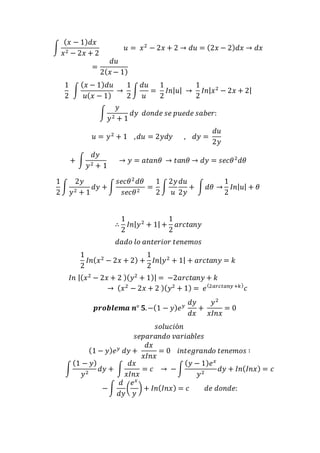
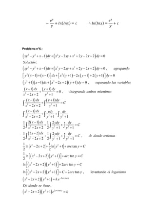
퐩퐫퐨퐛퐥퐞퐦퐚 퐧°ퟒ. −(푥푦2 − 푦2 + 푥 − 1)푑푥 + (푥2 푦) − 2푥푦 + 푥2
+ 2푦 − 2푥 + 2)푑푦 = 0
푠표푙푢푐푖ó푛:
푎푔푟푢푝푎푛푑표 푡é푟푚푖푛표푠 푡푒푛푒푚표푠:
[푦2 (푥 − 1) + (푥 − 1)]푑푥 + [푦(푥2 − 2푥 + 2)]푑푦 = 0
푓푎푐푡표푟푖푧푎푛푑표 푡푒푛푒푚표푠:
(푦2 + 1)(푥 − 1)푑푥 + (푦 + 1)(푥2 − 2푥) + 2푑푦 = 0
푠푒푝푎푟푎푛푑표 푙푎푠 푣푎푟푖푎푏푙푒푠
(푥 + 1)푑푥
푥2 − 2푥 + 2
+
푦 + 1
푦2 + 1
푑푦 = 0 푖푛푡푒푔푟푎푛푑표
∫
(푥 + 1)푑푥
푥2 − 2푥 + 2
+ ∫
푦 + 1
푦2 + 1
푑푦 = 푘 푑푒 푑표푛푑푒](https://image.slidesharecdn.com/trabajodematematica2fvbfdbdbndb-141024230706-conversion-gate02/85/Problemas-de-Ecuaciones-Diferenciales-4-320.jpg)


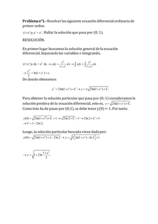
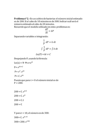
1) Se resuelve una ecuación diferencial ordinaria de primer orden encontrando primero la solución general e imponiendo la condición inicial para hallar la solución particular. 2) Se modela el crecimiento bacteriano mediante una ecuación diferencial y se calcula el número de bacterias a los 20 minutos usando las condiciones iniciales y la solución de la ecuación. 3) Se resuelve una ecuación diferencial parcial mediante separación de variables y se obtiene la solución general en términos de funciones logarítmicas y trigonométricas.


![La guerra del guano y el salitre todo[1]](https://cdn.slidesharecdn.com/ss_thumbnails/laguerradelguanoyelsalitretodo1-141205140249-conversion-gate02-thumbnail.jpg?width=640&height=640&fit=bounds)


